Applying L1 Trend Filtering in MetaTrader 5

MetaTrader 5 — Examples | 20 April 2026, 09:21

2 259

MetaQuotes

The primary goal of L1 trend filtering is to extract the underlying trend from a time series in such a way that:

long-term dynamics of the data are preserved;
short-term fluctuations and noise are suppressed;
structural breakpoints (changes in trend slope) are automatically detected.

Unlike classical smoothing methods, this approach does not enforce smoothness of the trend and instead produces a piecewise-linear approximation, which is particularly important for financial time series analysis.

L1 trend filtering

Contents

Introduction

Financial time series are characterized by high noise levels, frequent outliers, and changing market regimes. In practical trading systems, this manifests in a simple and measurable way: classical “smooth” filters (moving averages, HP) lag behind, blur the moments of slope changes, and often interpret local corrections as reversals — as a result, the number of false entries/exits increases, the Profit Factor decreases, and drawdown grows. In addition, the selection of the regularization parameter λ is usually reduced to manual tuning and does not transfer well across instruments, timeframes, and history lengths.

This paper proposes a practical solution to these problems based on L1 trend filtering: optimization with L1 regularization of second differences automatically produces a piecewise-linear approximation with explicit breakpoints. The key advantages are a clear interpretation of breakpoints as regime changes, the ability to set the scale of regularization via computing λmax and moving to a relative parameter λ = coef · λmax, as well as linear computational complexity suitable for implementation in MQL5.

We present not only the theory, but also a complete practical roadmap: methods for computing λmax and the L1 trend, three indicators (trend, slope, slope sign), seven L1-trend volatility indicators, integration into Expert Advisors, and a reproducible testing protocol (four filtering modes, balance/equity export, and visualization).

1. Formulation of the Trend Filtering Problem

We consider a scalar time series represented as the sum of two components:

where is the trend component, and is a noise or an irregular component.

The objective is to estimate the trend from the observed data .

The problem can be expressed as a trade-off between fidelity to the original data and smoothness of the estimated trend.

1.1. Hodrick–Prescott Filter

The Hodrick–Prescott filter defines the trend as the solution to the minimization problem:

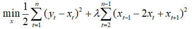where the parameter λ controls the degree of smoothing.

Main properties of the HP filter:

Linearity with respect to the data;
Computational complexity O(n);
For small λ, the trend approximates the original data;
For large λ, the trend tends to the best linear approximation.

However, the HP filter always produces a smooth trend and poorly detects sharp changes in slope.

1.2. L1 Trend Filtering Method

The main idea of L1 trend filtering is to find a trend that is close to the original data but contains as few changes in slope as possible. Unlike classical smoothing methods that minimize the squared curvature, the L1 approach minimizes the sum of absolute values of second differences.

This leads to a fundamentally different result:

most second differences become equal to zero,
the trend is automatically split into linear segments.

Thus, the L1 filter does not attempt to make the trend smooth but instead finds the minimal number of structural changes that explain the observed data. This makes the method particularly suitable for financial time series, where dynamics often consist of sequences of quasi-linear growth and decline phases.

In L1 trend filtering, the quadratic penalty on second differences is replaced by the L1 norm, and the trend is defined as the solution to a convex optimization problem:

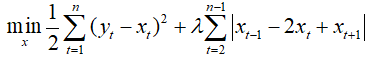
In matrix form:

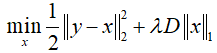
where:

y — input time series;
x — the estimated trend;
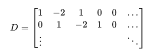
D — second-difference matrix;
λ>=0 — regularization parameter.

The use of the L1 norm leads to a fundamentally different result: many second differences become zero, meaning that the trend is piecewise linear.

The second difference is defined as:

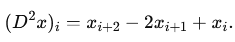
If , then the points lie on a straight line.

Therefore, a zero second difference corresponds to a linear segment of the trend, while a nonzero second difference corresponds to a breakpoint. The L1 norm promotes sparsity in the vector Dx, meaning that most second differences become zero. This implies that over the corresponding intervals, the trend is linear. Points where second differences are nonzero are interpreted as trend breakpoints.

Thus, the L1 Trend Filtering method automatically constructs the trend as a set of linear segments connected at points of structural change.

Main properties of L1 trend filtering:

The trend consists of linear segments;
Breakpoints are interpreted as structural changes in the time series;
At λ = 0, the trend coincides with the original data;
For sufficiently large λ, the trend becomes exactly the best linear approximation;
Computational complexity remains linear in the number of observations.

1.3. Role of the Regularization Parameter λ

The parameter λ controls the trade-off between approximation accuracy and trend complexity:

Value of λ	Nature of the solution
λ=0	x=y, no smoothing
Small λ	Weak smoothing, many breakpoints
Medium λ	Piecewise-linear trend
Large λ	Nearly linear trend
λ≥λmax	Strictly linear trend

Table 1. Dependence of the L1 trend on the regularization parameter λ

Thus, λ controls the number and locations of trend breakpoints.

1.4. Geometric Interpretation of the Problem

The desired trend x can be viewed as a point in an n-dimensional space. The first term of the objective function, responsible for approximation accuracy, defines a Euclidean ball centered at the observation point y: the closer x is to y, the smaller the error.

The regularization term with the L1 norm of second differences defines a convex polyhedral set (polyhedron). Unlike smooth ellipsoids arising in L2 regularization, this polyhedron has sharp vertices. These vertices correspond to situations where some second differences of the trend are equal to zero.

It is precisely the presence of sharp corners in the L1 norm that leads to sparse solutions: the optimal solution tends to lie at a vertex of the polyhedron, where only some constraints are active. This means that most second differences become zero, and the trend automatically takes a piecewise-linear form.

The optimal solution corresponds to the first point of contact between the Euclidean ball and the L1 polyhedron. At this point, the trend consists of linear segments connected at a limited number of breakpoints.

The parameter λmax corresponds to the situation where the Euclidean ball touches the L1 polyhedron not at a vertex but along the subspace of linear functions. In this case, all second differences are zero, and the trend is strictly linear.

For λ ≥ λmax, none of the L1 constraints become active, so further increases in regularization do not change the solution, and the trend remains linear.

1.5. Algorithm for Computing λmax

Consider the computation of the maximum regularization parameter λmax for an input vector y of length N.

1. Construct the second-difference matrix D of size (N−2)×N:

2. Compute the curvature vector Dy.

3. Solve the system of linear equations:

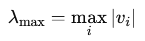
4. Take the maximum (by absolute value) element of vector v:

For financial time series, the parameter λmax has important practical significance:

It allows normalization of the regularization parameter;
It makes the choice of λ independent of the data scale;
It simplifies comparison across different time series;
It allows interpreting λ as a fraction of the maximum regularization.

Using a relative parameter of the form: λ=coef_lambda_max⋅λmax⁡, where coef_lambda_max ∈ (0,1), greatly simplifies practical application.

In the following examples of indicators and Expert Advisors, λ will be used in units of λmax, while the parameter settings will specify the multiplier coef_lambda_max.

2. MQL5 Methods for Calculation the L1 Trend

For practical use of L1 trend filtering, two methods are implemented for vectors of type double and float.

L1TrendFilterLambdaMax computes the maximum regularization parameter;
L1TrendFilter computes the L1 trend for a given value of the regularization parameter λ, which can also be specified in units of λmax.

2.1. L1TrendFilterLambdaMax

Method for calculation the maximum regularization parameter λmax for a data vector.

Calculation for vector<double>:

bool  vector::L1TrendFilterLambdaMax(
   double          &lambda_max       // the maximum value of the regularization parameter lambda
   )

Calculation for vector<float>:

bool  vectorf::L1TrendFilterLambdaMax(
   float           &lambda_max       // the maximum value of the regularization parameter lambda
   );

Parameters

lambda

[out] The maximum value of the regularization parameter λmax, or -1 in case of an error.

Return value

Returns true if successful.

Note

Memory consumption grows linearly with the vector size.

2.2. L1TrendFilter

Method for calculation the L1 trend for a data vector.

Calculation for vector<double>:

bool  vector::L1TrendFilter(
   double          lambda,         // regularization parameter
   bool            relative,       // flag indicating lambda is in λmax units
   vector&         result          // output vector with L1 filtering result
   );

Calculation for vector<float>:

bool  vectorf::L1TrendFilter(
   float           lambda,         // regularization parameter
   bool            relative,       // flag indicating lambda is in λmax units
   vectorf&        result          // output vector with L1 filtering result
   );

Parameters

lambda

[in] Value of the regularization parameter lambda (if relative = true the lambda is defined in range [0, 1] as fraction of λmax).

relative

[in] Flag indicating how λ is specified. If true, λ is given in units of λmax; otherwise, the absolute value is used.

result

[out] Vector containing the result of L1 filtering.

Return value

Returns true if successful.

Note

Memory consumption grows linearly with the vector size.

Recommended ranges for λ (relative mode).

λ multiplier	Result
0.005 – 0.015	almost L2, noisy
0.02 – 0.04	micro-segments
0.04 – 0.07	optimal for signals
0.07 – 0.12	medium-term trends
0.12 – 0.25	market regimes
> 0.3	few segments

Table.2. Working ranges of λ in units of λmax⁡

For practical applications, it is recommended to use multipliers in the range 0.04–0.25.

3. Examples of Application

In this section, we consider L1 trend calculations on simulated Brownian motion data, on S&P 500 price data, as well as scaling properties of λmax for both Brownian motion and FOREX market data.

We also present three indicator variants that help determine optimal regularization parameters (multipliers of λmax) for obtaining the best L1 trend decomposition for specific symbols and timeframes.

Additionally, results of filtering trading signals (alignment with the L1 trend) are presented for the MovingAverage, MACD, ADX, and EMA strategies.

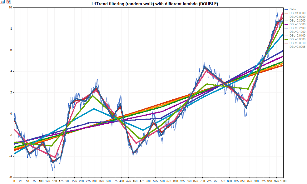
3.1. L1 Trend Calculation on Simulated Data (Random Walk)

As an example, consider computing the L1 trend with different values of the regularization parameter λ on simulated Brownian motion data.

Script code:

//+------------------------------------------------------------------+
//|                                                  TestL1Trend.mq5 |
//|                             Copyright 2000-2026, MetaQuotes Ltd. |
//|                                              http://www.mql5.com |
//+------------------------------------------------------------------+
#property copyright "Copyright 2000-2026, MetaQuotes Ltd."
#property link      "https://www.mql5.com"
#property version   "1.00"
#property script_show_inputs
#include <Graphics\Graphic.mqh>
//+------------------------------------------------------------------+
//| Generate Brown movement data                                     |
//+------------------------------------------------------------------+
void BMData(vector<double> &data,int &data_count)
  {
   data.Resize(data_count);
   data[0] = 0.0;
   for(int i=1; i<data_count; i++)
      data[i] = data[i-1] + (MathRand()/32767.0 - 0.5);
  }
//+------------------------------------------------------------------+
//| CopyValues                                                       |
//+------------------------------------------------------------------+
bool CopyValues(vector<double> &data_v,double &data[])
  {
   int data_count=(int)data.Size();
   if(data_count==0)
      return(false);
   ArrayResize(data,data.Size());
   for(int i=0; i<data_count; i++)
      data[i]=data_v[i];
   return(true);
  }
//+------------------------------------------------------------------+
//| Script program start function                                    |
//+------------------------------------------------------------------+
void OnStart()
  {
   MathSrand(1);
   int data_count=1000;
   vector<double> data_test;
   BMData(data_test,data_count);
//--- prepare arrays for chart
   double x[],y[];
   ArrayResize(x,data_count);
   ArrayResize(y,data_count);
   for(int i=0; i<data_count; i++)
      x[i]=i;
//---
   CGraphic graphic;
   long chart=0;
   string name="test";
   if(ObjectFind(chart,name)<0)
      graphic.Create(chart,name,0,0,0,1000,600);
   else
      graphic.Attach(chart,name);
   graphic.BackgroundMain("L1 Trend filtering (random walk) with different lambda");
   graphic.BackgroundMainSize(16);
   graphic.HistoryNameWidth(60);
   graphic.HistoryColor(ColorToARGB(clrGray,255));
   graphic.XAxis().AutoScale(false);
   graphic.XAxis().Min(0);
   graphic.XAxis().Max(data_count);
//---
   CopyValues(data_test,y);
   graphic.CurveAdd(x,y,CURVE_LINES,"Data").LinesWidth(1);
//--- L1TrendFilterLambdaMax
   double lambda_max=0.0;
   if(data_test.L1TrendFilterLambdaMax(lambda_max))
      PrintFormat("lambda_max=%f",lambda_max);
//---
   vector<double> data_l1;
   const double lambda_factors[]= {1.0,0.9,0.8,0.5,0.25,0.1,0.01,0.05,0.001,0.0005};
   for(int i=0; i<ArraySize(lambda_factors); i++)
     {
      double lambda=lambda_max*lambda_factors[i];
      PrintFormat("%d. lambda=%f",i+1,lambda);
      bool res=data_test.L1TrendFilter(lambda_factors[i],true,data_l1);
      if(res)
        {
         CopyValues(data_l1,y);
         graphic.CurveAdd(x,y,CURVE_LINES,"lambda="+DoubleToString(lambda,0)).LinesWidth(3);
        }
     }
//---
   graphic.CurvePlotAll();
   graphic.Update();
   DebugBreak();
  }
//+------------------------------------------------------------------+

Output:

TestL1Trend (EURUSD,H1) lambda_max=51703.353749
TestL1Trend (EURUSD,H1) 1. lambda=51703.353749
TestL1Trend (EURUSD,H1) 2. lambda=46533.018374
TestL1Trend (EURUSD,H1) 3. lambda=41362.682999
TestL1Trend (EURUSD,H1) 4. lambda=25851.676874
TestL1Trend (EURUSD,H1) 5. lambda=12925.838437
TestL1Trend (EURUSD,H1) 6. lambda=5170.335375
TestL1Trend (EURUSD,H1) 7. lambda=517.033537
TestL1Trend (EURUSD,H1) 8. lambda=2585.167687
TestL1Trend (EURUSD,H1) 9. lambda=51.703354
TestL1Trend (EURUSD,H1) 10. lambda=25.851677

In this example, it can be seen that decreasing the regularization parameter λ allows for a more detailed decomposition into trend segments (Fig.1).

If λ ≥ λmax, the solution becomes a straight line corresponding to linear regression (the global trend).

Fig.1. Example of L1 filter computation with different values of λ on Brownian motion data

Functions for computing the L1 trend are available for both double and float vectors.

Test script for comparing the calculations is presented below.

//+------------------------------------------------------------------+
//|                                       TestL1TrendFloatDouble.mq5 |
//|                             Copyright 2000-2026, MetaQuotes Ltd. |
//|                                              http://www.mql5.com |
//+------------------------------------------------------------------+
#property copyright "Copyright 2000-2026, MetaQuotes Ltd."
#property link      "https://www.mql5.com"
#property version   "1.00"

#include <Graphics\Graphic.mqh>

uint32_t ExtSeed=1;
//+------------------------------------------------------------------+
//| Generate Brown movement data                                     |
//+------------------------------------------------------------------+
template<typename T>
void BMData(vector<T> &data,uint64_t data_count)
  {
   MathSrand(ExtSeed);

   data.Resize(data_count);
   data[0] = 0.0;

   for(uint64_t i=1; i<data_count; i++)
      data[i] = data[i-1] + T(MathRand()/32767.0 - 0.5);
  }
//+------------------------------------------------------------------+
//| CopyValues                                                       |
//+------------------------------------------------------------------+
template<typename T>
bool CopyValues(double &data[],const vector<T> &data_v)
  {
   if(ArrayResize(data,data.Size())!=data.Size())
      return(false);
   for(uint64_t i=0; i<data.Size(); i++)
      data[i]=data_v[i];

   return(true);
  }
//+------------------------------------------------------------------+
//| L1TrendCalculate                                                 |
//+------------------------------------------------------------------+
template<typename T>
bool L1TrendCalculate(double &result[],uint64_t data_count,double lambda,bool lambda_is_relative)
  {
   vector<T> data_test;
   BMData(data_test,data_count);

   vector<T> vres;
   if(!data_test.L1TrendFilter((T)lambda,lambda_is_relative,vres))
      return(false);
   if(ArrayResize(result,(uint32_t)vres.Size())!=vres.Size())
      return(false);
   for(uint64_t n=0; n<result.Size(); n++)
      result[n]=vres[n];

   return(true);
  }
//+------------------------------------------------------------------+
//| TestRun                                                          |
//+------------------------------------------------------------------+
bool TestRun(uint32_t data_count,uint32_t mode)
  {
//--- create graph
   CGraphic graphic;
   long     chart=0;
   string   name="L1TrendTest";

   if(ObjectFind(chart,name)<0)
      graphic.Create(chart,name,0,0,0,1280,600);
   else
      graphic.Attach(chart,name);

   string mode_name="(";
   if((mode&1)==1)
      mode_name+="DOUBLE";
   if((mode&3)==3)
      mode_name+=" & ";
   if((mode&2)==2)
      mode_name+="FLOAT";
   mode_name+=")";

   graphic.BackgroundMain("L1Trend filtering (random walk) with different lambda "+mode_name);
   graphic.BackgroundMainSize(16);
   graphic.HistoryNameWidth(60);
   graphic.HistoryColor(ColorToARGB(clrGray,255));
   graphic.XAxis().AutoScale(false);
   graphic.XAxis().Min(0);
   graphic.XAxis().Max(data_count);
//--- prepare arrays
   double x[];
   double y[];

   if(ArrayResize(x,data_count)!=data_count)
      return(false);
  
   for(uint32_t i=0; i<data_count; i++)
      x[i]=i;

   vector<double> v;
   BMData(v,data_count);
   v.Swap(y);
   graphic.CurveAdd(x,y,CURVE_LINES,"Data").LinesWidth(1);
//--- calculate
   const double lambda_factors[]= {1.0,0.9,0.8,0.5,0.25,0.1,0.01,0.05,0.001,0.0005};
//--- double
   if((mode&1)==1)
     {
      for(uint64_t i=0; i<lambda_factors.Size(); i++)
        {
         if(L1TrendCalculate<double>(y,data_count,lambda_factors[i],true))
            graphic.CurveAdd(x,y,CURVE_LINES,"DBL="+DoubleToString(lambda_factors[i],4)).LinesWidth(4);
        }
     }
//--- float
   if((mode&2)==2)
     {
      for(uint64_t i=0; i<lambda_factors.Size(); i++)
        {
         if(L1TrendCalculate<float>(y,data_count,(float)lambda_factors[i],true))
            graphic.CurveAdd(x,y,CURVE_LINES,"FLT="+DoubleToString(lambda_factors[i],4)).LinesWidth(2);
        }
     }
//--- update
   graphic.CurvePlotAll();
   graphic.Update();
   return(true);
  }
//+------------------------------------------------------------------+
//| Script program start function                                    |
//+------------------------------------------------------------------+
void OnStart()
  {
   for(uint32_t n=0; !IsStopped(); n++,Sleep(1000))
     {
      TestRun(1000,1+n%3);

      if((n%3)==2)
         ExtSeed++;
     }
  }
//+------------------------------------------------------------------+

Output:

3.2. L1 Trend Calculation for S&P 500 Price Series

Consider the computation of log(S&P 500) from the original paper l_1 Trend Filtering, S.J. Kim, K. Koh, S. Boyd, and D. Gorinevsky, SIAM Review, problems and techniques section, 51(2):339–360, May 2009.

To run the script, data from the file "snp500.txt" is used. It must be placed in the folder: terminal_data_folder\MQL5\Files

//+------------------------------------------------------------------+
//|                                       TestL1TrendFilterSP500.mq5 |
//|                             Copyright 2000-2026, MetaQuotes Ltd. |
//|                                              http://www.mql5.com |
//+------------------------------------------------------------------+
#property copyright "Copyright 2000-2026, MetaQuotes Ltd."
#property link      "https://www.mql5.com"
#property version   "1.00"
#property script_show_inputs
#include <Graphics\Graphic.mqh>
//+------------------------------------------------------------------+
//| LoadData                                                         |
//+------------------------------------------------------------------+
void LoadData(string filename,vector<double> &data,int &data_count)
  {
   data_count=0;
   ResetLastError();
   int file_handle=FileOpen(filename,FILE_READ|FILE_TXT|FILE_ANSI);
   if(file_handle!=INVALID_HANDLE)
     {
      while(!FileIsEnding(file_handle))
        {
         string str=FileReadString(file_handle);
         if(data.Size()<=(ulong)data_count)
            data.Resize(data_count+1);
         data[data_count]=StringToDouble(str);
         data_count++;
        }
      FileClose(file_handle);
     }
   else
      PrintFormat("Failed to open %s file, Error code = %d",filename,GetLastError());
//---
   data.Resize(data_count);
  }
//+------------------------------------------------------------------+
//| Script program start function                                    |
//+------------------------------------------------------------------+
void OnStart()
  {
   long chart=0;
   string name="log SP500";
   int data_count=0;
   vector<double> data_sp500;
   LoadData("snp500.txt",data_sp500,data_count);
   vector<double> data_l1_sp500;
   data_l1_sp500.Resize(data_count);
//--- L1TrendFilterLambdaMax
   double lambda_max=0.0;
   if(data_sp500.L1TrendFilterLambdaMax(lambda_max))
      PrintFormat("Lambda_max=%f",lambda_max);
   double lambda=50;
//--- L1TrendFilter
   if(data_sp500.L1TrendFilter(lambda,false,data_l1_sp500))
     {
      //--- prepare arrays for chart
      double x[],y[],y2[];
      ArrayResize(x,data_count);
      ArrayResize(y,data_count);
      ArrayResize(y2,data_count);
      for(int i=0; i<data_count; i++)
        {
         x[i]=i;
         y[i]=data_sp500[i];
         y2[i]=data_l1_sp500[i];
        }
      //---
      CGraphic graphic;
      if(ObjectFind(chart,name)<0)
         graphic.Create(chart,name,0,0,0,1000,600);
      else
         graphic.Attach(chart,name);
      graphic.BackgroundMain("log SP500 L1 trend filtering");
      graphic.BackgroundMainSize(16);
      graphic.HistoryNameWidth(60);
      graphic.HistoryColor(ColorToARGB(clrGray,255));
      graphic.XAxis().AutoScale(false);
      graphic.XAxis().Min(0);
      graphic.XAxis().Max(data_count);
      graphic.XAxis().DefaultStep(100);
      graphic.CurveAdd(x,y,CURVE_LINES,"SP500").LinesWidth(1);
      graphic.CurveAdd(x,y2,CURVE_LINES,"L1 trend").LinesWidth(3);
      graphic.CurvePlotAll();
      graphic.Update();
      DebugBreak();
     }
  }
//+------------------------------------------------------------------+

The result of the script execution is shown in Fig.2.

Fig.2. Example of L1-trend estimation for log price series of the S&P 500 index

In the Experts tab, the value of λmax for the given time series will be displayed:

TestL1TrendFilterSP500 (EURUSD,H1)      Lambda_max=37394.835512

This script demonstrates the use of the methods L1TrendFilterLambdaMax and L1TrendFilter with a fixed value λ = 50, as in the original paper by the method’s authors.

In the following examples, instead of absolute values of the regularization parameter λ, relative values (in units of λmax) will be used with the flag relative = true.

3.3. Scaling Properties of λmax⁡

The parameter λmax plays a key role in L1 filtering, as it defines the upper bound of regularization at which the solution degenerates into a global linear approximation. An interesting property of this quantity is its scaling dependence on the length of the time series.

Numerical experiments show that λmax grows according to a power law with respect to the number of observations:

where: T — length of the time series, α — scaling exponent.

For a random walk (Brownian motion), it can be shown that the exponent should be close to α ≈ 2.5. The amplitude of Brownian motion grows as

, while the second-difference operator scales as

. In computing λmax, one effectively evaluates the maximum of a quantity related to the integral of the curvature of the series.

As a result, the combined scaling leads to the relationship:

which corresponds to an exponent α ≈ 2.5.

Thus, as the length of the time series increases, the value of λmax grows significantly faster than linearly.

3.3.1. Numerical Experiment for Brownian Motion

To verify the scaling law, a numerical experiment was conducted.

For different time series lengths T, realizations of Brownian motion were generated, after which the average value of λmax was computed.

A logarithmic approximation was used:

which allows estimating the exponent α using linear regression.

The code for the experiment is given below.

//+------------------------------------------------------------------+
//|                            TestScalingLambdaMaxBrownMovement.mq5 |
//|                             Copyright 2000-2026, MetaQuotes Ltd. |
//|                                              http://www.mql5.com |
//+------------------------------------------------------------------+
#property copyright "Copyright 2000-2026, MetaQuotes Ltd."
#property link      "https://www.mql5.com"
#property version   "1.00"
#include <Graphics\Graphic.mqh>
//+------------------------------------------------------------------+
//| Generate Brownian motion                                         |
//+------------------------------------------------------------------+
void GenerateBrownian(int N,vector<double> &data)
  {
   data.Resize(N);
   data[0] = 0.0;
   for(int i=1; i<N; i++)
      data[i] = data[i-1] + (MathRand()/32767.0 - 0.5);
  }
//+------------------------------------------------------------------+
//| LinearRegression                                                 |
//+------------------------------------------------------------------+
void LinearRegression(const double &x[], const double &y[], int n, double &a, double &b)
  {
   double sx = 0.0, sy = 0.0, sxx = 0.0, sxy = 0.0;
   for(int i = 0; i < n; i++)
     {
      sx  += x[i];
      sy  += y[i];
      sxx += x[i] * x[i];
      sxy += x[i] * y[i];
     }
   double denom = n * sxx - sx * sx;
   a = (n * sxy - sx * sy) / denom;
   b = (sy - a * sx) / n;
  }
//+------------------------------------------------------------------+
//| TestScaling with statistics                                      |
//+------------------------------------------------------------------+
void TestScalingStatistics()
  {
   MathSrand(42);
   int RUNS = 10;     //
   int MC   = 10;   // Monte Carlo
   double alpha_values[];
   ArrayResize(alpha_values, RUNS);
// --- geometric grid of T
   int nT = 8;
   int Tvals[];
   ArrayResize(Tvals, nT);
   int T0 = 64;
   for(int i = 0; i < nT; i++)
      Tvals[i] = T0 << i;
   Print("Scaling test with statistics");
//---
   double logT[];
   double logLambda[];
   vector<double> bm;
   vector<double> l1_trend;
   for(int run = 0; run < RUNS; run++)
     {
      ArrayResize(logT, nT);
      ArrayResize(logLambda, nT);
      //---
      for(int i = 0; i < nT; i++)
        {
         int T = Tvals[i];
         double lambda_sum = 0.0;
         l1_trend.Resize(T);
         for(int k = 0; k < MC; k++)
           {
            GenerateBrownian(T, bm);
            double lambda_max=0.0;
            if (bm.L1TrendFilterLambdaMax(lambda_max))
               lambda_sum += lambda_max;
            bm.L1TrendFilter(0.2,true,l1_trend);
           }
         double lambda_avg = lambda_sum / MC;
         logT[i]      = MathLog((double)T);
         logLambda[i] = MathLog(lambda_avg);
        }
      // --- regression
      double alpha, c;
      LinearRegression(logT, logLambda, nT, alpha, c);
      alpha_values[run] = alpha;
      PrintFormat("run %d -> alpha = %.6f", run+1, alpha);
     }
//--- statistics
   double mean = 0.0;
   for(int i=0;i<RUNS;i++)
      mean += alpha_values[i];
   mean /= RUNS;
// --- standard deviation
   double var = 0.0;
   for(int i=0;i<RUNS;i++)
      var += (alpha_values[i]-mean)*(alpha_values[i]-mean);
   var /= (RUNS - 1);
   double stddev = MathSqrt(var);
// --- standard error of mean
   double sem = stddev / MathSqrt((double)RUNS);
// --- theoretical comparison
   double alpha_theory=2.5;
   double percent_error=MathAbs(mean-alpha_theory)/alpha_theory*100.0;
//--- results
   PrintFormat("mean alpha = %.6f", mean);
   PrintFormat("std deviation = %.6f", stddev);
   PrintFormat("standard error = %.6f", sem);
   PrintFormat("theory = %.4f", alpha_theory);
   PrintFormat("percent error from theory = %.4f %%", percent_error);
  }
//+------------------------------------------------------------------+
//| TestScaling                                                      |
//+------------------------------------------------------------------+
void TestScaling()
  {
   MathSrand(1);
// --- geometric grid of T
   int nT = 8;
   int Tvals[];
   ArrayResize(Tvals,nT);
//---
   int T0 = 64;
   for(int i=0; i<nT; i++)
      Tvals[i]=T0<<i;   // 64 * 2^i
//---
   double logT[], logLambda[];
   ArrayResize(logT,nT);
   ArrayResize(logLambda,nT);
//---
   Print("scaling test for lambda_max");
   for(int i=0; i<nT; i++)
     {
      int T = Tvals[i];
      //--- Monte-Carlo simulations
      int MC=1000;
      double lambda_sum = 0.0;
      for(int k=0; k<MC; k++)
        {
         vector<double> bm;
         GenerateBrownian(T, bm);
         double lambda_max=0.0;
         if(bm.L1TrendFilterLambdaMax(lambda_max))
            lambda_sum += lambda_max;
        }
      double lambda_avg=lambda_sum/MC;
      logT[i]= MathLog((double)T);
      logLambda[i]=MathLog(lambda_avg);
      PrintFormat("T=%5d   <lambda_max>=%.6f",T,lambda_avg);
     }
// --- linear regression in log-log
   double alpha, c;
   LinearRegression(logT,logLambda,nT,alpha,c);
//---
   PrintFormat("estimated scaling exponent alpha = %.4f",alpha);
   double alpha_theory=2.5;
   PrintFormat("theoretical value = %.4f",alpha_theory);
//--- plot scaling law
   CGraphic g;
   g.Create(0, "ScalingLaw",0,0,0,1000,600);
   g.BackgroundMain("Scaling law of lambda_max (Brownian motion)");
   g.BackgroundMainSize(16);
   g.CurveAdd(logT, logLambda, CURVE_POINTS, "Simulation");
//---
   double xfit[2], yfit[2];
   xfit[0] = logT[0];
   xfit[1] = logT[nT-1];
//---
   yfit[0] = alpha*xfit[0] + c;
   yfit[1] = alpha*xfit[1] + c;
//---least squares fit
   g.CurveAdd(xfit, yfit, CURVE_LINES, "LS fit");
   g.CurvePlotAll();
   g.Update();
   DebugBreak();
  }
//+------------------------------------------------------------------+
//| Script program start function                                    |
//+------------------------------------------------------------------+
void OnStart()
  {
//--- calculate scaling with statistics
   TestScalingStatistics();
//--- show sample results
   TestScaling();
  }
//+------------------------------------------------------------------+

Output:

TestScalingLambdaMaxBrownMovement (EURUSD,H1)   Scaling test with statistics    
TestScalingLambdaMaxBrownMovement (EURUSD,H1)   run 1 -> alpha = 2.480774       
TestScalingLambdaMaxBrownMovement (EURUSD,H1)   run 2 -> alpha = 2.530977       
TestScalingLambdaMaxBrownMovement (EURUSD,H1)   run 3 -> alpha = 2.435511       
TestScalingLambdaMaxBrownMovement (EURUSD,H1)   run 4 -> alpha = 2.461984       
TestScalingLambdaMaxBrownMovement (EURUSD,H1)   run 5 -> alpha = 2.467093       
TestScalingLambdaMaxBrownMovement (EURUSD,H1)   run 6 -> alpha = 2.487965       
TestScalingLambdaMaxBrownMovement (EURUSD,H1)   run 7 -> alpha = 2.532371       
TestScalingLambdaMaxBrownMovement (EURUSD,H1)   run 8 -> alpha = 2.455831       
TestScalingLambdaMaxBrownMovement (EURUSD,H1)   run 9 -> alpha = 2.483485       
TestScalingLambdaMaxBrownMovement (EURUSD,H1)   run 10 -> alpha = 2.420283      
TestScalingLambdaMaxBrownMovement (EURUSD,H1)   mean alpha = 2.475627   
TestScalingLambdaMaxBrownMovement (EURUSD,H1)   std deviation = 0.036281        
TestScalingLambdaMaxBrownMovement (EURUSD,H1)   standard error = 0.011473       
TestScalingLambdaMaxBrownMovement (EURUSD,H1)   theory = 2.5000 
TestScalingLambdaMaxBrownMovement (EURUSD,H1)   percent error from theory = 0.9749 %    
TestScalingLambdaMaxBrownMovement (EURUSD,H1)   scaling test for lambda_max     
TestScalingLambdaMaxBrownMovement (EURUSD,H1)   T=   64   <lambda_max>=97.302362        
TestScalingLambdaMaxBrownMovement (EURUSD,H1)   T=  128   <lambda_max>=566.626861       
TestScalingLambdaMaxBrownMovement (EURUSD,H1)   T=  256   <lambda_max>=3162.076116      
TestScalingLambdaMaxBrownMovement (EURUSD,H1)   T=  512   <lambda_max>=18271.204936     
TestScalingLambdaMaxBrownMovement (EURUSD,H1)   T= 1024   <lambda_max>=100057.796790    
TestScalingLambdaMaxBrownMovement (EURUSD,H1)   T= 2048   <lambda_max>=578620.887399    
TestScalingLambdaMaxBrownMovement (EURUSD,H1)   T= 4096   <lambda_max>=3192555.936035   
TestScalingLambdaMaxBrownMovement (EURUSD,H1)   T= 8192   <lambda_max>=17895314.647170  
TestScalingLambdaMaxBrownMovement (EURUSD,H1)   estimated scaling exponent alpha = 2.4967       
TestScalingLambdaMaxBrownMovement (EURUSD,H1)   theoretical value = 2.5000

The double-log plot (in double-logarithmic scale) shows the presence of a power-law dependence of the function λmax on the number of data points for Brownian motion.
.

Fig.3. Power-law dependence of LambdaMax for Brownian motion

The simulation results show:

mean alpha = 2.4756
std deviation = 0.036
theory = 2.5
percent error ≈ 1%

Thus, the experiment confirms the theoretical relationship:

The double-log plot in double-logarithmic scale demonstrates a linear relationship between log(λmax) and log(T).

3.3.2. Scaling for financial time series

A similar experiment was conducted for FOREX market price series. For different currency pairs and timeframes, the exponent α was estimated.

The results show that for real financial data the value of α also lies in the range α ≈ 2.45–2.60, which is very close to the theoretical value for Brownian motion. This means that the scaling behavior of λmax is nearly universal and holds across different markets and timeframes.

The script TestScalingLambdaMaxSymbol.mq5 computes the exponent of λmax for a given symbol across standard timeframes M1–H1.

//+------------------------------------------------------------------+
//|                                   TestScalingLambdaMaxSymbol.mq5 |
//|                             Copyright 2000-2026, MetaQuotes Ltd. |
//|                                              http://www.mql5.com |
//+------------------------------------------------------------------+
#property copyright "Copyright 2000-2026, MetaQuotes Ltd."
#property link      "https://www.mql5.com"
#property version   "1.00"
#property script_show_inputs
//--- input parameters
input string WorkSymbol   = "EURUSD";     // Symbol
input int    YearStart    = 2024;
input int    YearEnd      = 2025;
#include <Graphics\Graphic.mqh>
//+------------------------------------------------------------------+
//| GetHistoricalData                                                |
//+------------------------------------------------------------------+
bool GetHistoricalData(double &data[], string symbol, ENUM_TIMEFRAMES tf, int year_start, int year_end)
  {
   datetime from = StringToTime(IntegerToString(year_start) + ".01.01 00:00");
   datetime to   = StringToTime(IntegerToString(year_end)   + ".12.31 23:59");
   int copied = CopyClose(symbol, tf, from, to, data);
   if(copied <= 0)
     {
      Print("Error in CopyClose: ", GetLastError());
      ArrayResize(data, 0);
      return false;
     }
//PrintFormat("Loaded bars: %d (%s %s)", ArraySize(data), symbol, EnumToString(tf));
   return true;
  }
//+------------------------------------------------------------------+
//| LinearRegression                                                 |
//+------------------------------------------------------------------+
void LinearRegression(const double &x[], const double &y[], int n, double &a, double &b)
  {
   double sx = 0, sy = 0, sxx = 0, sxy = 0;
   for(int i = 0; i < n; i++)
     {
      sx  += x[i];
      sy  += y[i];
      sxx += x[i] * x[i];
      sxy += x[i] * y[i];
     }
   double denom = n*sxx - sx*sx;
   if(denom!=0)
     {
      a = (n*sxy-sx*sy)/denom;
      b = (sy-a*sx)/n;
     }
  }
//+------------------------------------------------------------------+
//| Scaling test for one timeframe                                   |
//+------------------------------------------------------------------+
bool TestScalingLambaMaxTF(string symbol, ENUM_TIMEFRAMES tf, double &logT_out[], double &logLambda_out[], double &alpha_out)
  {
   MathSrand(42);
   double prices[];
   if(!GetHistoricalData(prices, symbol, tf, YearStart, YearEnd))
      return false;
   int Tvals[];
   int nT=8;
   int T0=64;
   ArrayResize(Tvals, nT);
   for(int i = 0; i < nT; i++)
      Tvals[i] = T0 << i;
   ArrayResize(logT_out, nT);
   ArrayResize(logLambda_out, nT);
   int data_size = ArraySize(prices);
   vector<double> data_prices;
   for(int i = 0; i < nT; i++)
     {
      int T = Tvals[i];
      int MC = 1000;
      double lambda_sum = 0.0;
      for(int k = 0; k < MC; k++)
        {
         if(data_size < T)
            break;
         int start = MathRand() % (data_size - T);
         data_prices.Resize(T);
         for(int j=0; j<T;  j++)
            data_prices[j]=prices[start+j];
         double lambda_max=0.0;
         if(data_prices.L1TrendFilterLambdaMax(lambda_max))
            lambda_sum += lambda_max;
        }
      double lambda_avg = lambda_sum / MC;
      logT_out[i]=MathLog((double)T);
      logLambda_out[i]=MathLog(lambda_avg);
      //PrintFormat("TF=%s T=%5d   <lambda_max>=%.6f", EnumToString(tf), T, lambda_avg);
     }
   double c;
   LinearRegression(logT_out, logLambda_out, nT, alpha_out, c);
   PrintFormat("%s (%s) estimated scaling exponent = %.4f", symbol,EnumToString(tf), alpha_out);
   return true;
  }
//+------------------------------------------------------------------+
//| TestScalingLambdaMaxSymbol                                       |
//+------------------------------------------------------------------+
void TestScalingLambdaMaxSymbol(string symbol)
  {
   ENUM_TIMEFRAMES timeframes[] = {PERIOD_M1, PERIOD_M2, PERIOD_M3, PERIOD_M4, PERIOD_M5, PERIOD_M6,
                                   PERIOD_M10, PERIOD_M12, PERIOD_M15, PERIOD_M20, PERIOD_M30, PERIOD_H1
                                  };
   uint colors[] = {clrRed,clrBlue,clrGreen,clrOrange,clrPurple,clrDarkGreen,clrCyan,
                    clrNavy,clrOrangeRed,clrDodgerBlue,clrCrimson,clrDarkRed
                   };
//---
   CGraphic g;
   g.Create(0,"ScalingLawTest",0,0,0,1000,600);
   g.BackgroundMain("Scaling law of lambda_max ("+symbol+")");
   g.BackgroundMainSize(16);
   PrintFormat("%s scaling test for standard timeframes",symbol);
   for(int i = 0; i < ArraySize(timeframes); i++)
     {
      double logT[], logLambda[], alpha;
      // Print("processing timeframe: ", EnumToString(timeframes[i]), " -----");
      if(TestScalingLambaMaxTF(symbol,timeframes[i],logT,logLambda,alpha))
        {
         g.CurveAdd(logT,logLambda,ColorToARGB(colors[i % ArraySize(colors)],255),CURVE_POINTS_AND_LINES,EnumToString(timeframes[i]));
        }
     }
   g.CurvePlotAll();
   g.Update();
//---
   DebugBreak();
  }
//+------------------------------------------------------------------+
//| Script program start function                                    |
//+------------------------------------------------------------------+
void OnStart()
  {
//--- estimate lambda_max scale exponent for price data
   TestScalingLambdaMaxSymbol(WorkSymbol);
  }
//+------------------------------------------------------------------+

Results for EURUSD:

TestScalingLambdMaxSymbol (EURUSD,H1)   EURUSD scaling test for standard timeframes     
TestScalingLambdMaxSymbol (EURUSD,H1)   EURUSD (PERIOD_M1) estimated scaling exponent = 2.5038  
TestScalingLambdMaxSymbol (EURUSD,H1)   EURUSD (PERIOD_M2) estimated scaling exponent = 2.5350  
TestScalingLambdMaxSymbol (EURUSD,H1)   EURUSD (PERIOD_M3) estimated scaling exponent = 2.5034  
TestScalingLambdMaxSymbol (EURUSD,H1)   EURUSD (PERIOD_M4) estimated scaling exponent = 2.5422  
TestScalingLambdMaxSymbol (EURUSD,H1)   EURUSD (PERIOD_M5) estimated scaling exponent = 2.5341  
TestScalingLambdMaxSymbol (EURUSD,H1)   EURUSD (PERIOD_M6) estimated scaling exponent = 2.5132  
TestScalingLambdMaxSymbol (EURUSD,H1)   EURUSD (PERIOD_M10) estimated scaling exponent = 2.5188 
TestScalingLambdMaxSymbol (EURUSD,H1)   EURUSD (PERIOD_M12) estimated scaling exponent = 2.5126 
TestScalingLambdMaxSymbol (EURUSD,H1)   EURUSD (PERIOD_M15) estimated scaling exponent = 2.5208 
TestScalingLambdMaxSymbol (EURUSD,H1)   EURUSD (PERIOD_M20) estimated scaling exponent = 2.4887 
TestScalingLambdMaxSymbol (EURUSD,H1)   EURUSD (PERIOD_M30) estimated scaling exponent = 2.5695 
TestScalingLambdMaxSymbol (EURUSD,H1)   EURUSD (PERIOD_H1) estimated scaling exponent = 2.6118

The results for EURUSD (standard timeframes M1–H1) are shown in Fig. 4.

Fig.4. Power-law dependence of λmax for the different EURUSD timeframes

Similarly, other currency pairs can be analyzed.

For USDJPY:

TestScalingLambdMaxSymbol (EURUSD,H1)   USDJPY scaling test for standard timeframes     
TestScalingLambdMaxSymbol (EURUSD,H1)   USDJPY (PERIOD_M1) estimated scaling exponent = 2.5851  
TestScalingLambdMaxSymbol (EURUSD,H1)   USDJPY (PERIOD_M2) estimated scaling exponent = 2.5825  
TestScalingLambdMaxSymbol (EURUSD,H1)   USDJPY (PERIOD_M3) estimated scaling exponent = 2.4889  
TestScalingLambdMaxSymbol (EURUSD,H1)   USDJPY (PERIOD_M4) estimated scaling exponent = 2.5099  
TestScalingLambdMaxSymbol (EURUSD,H1)   USDJPY (PERIOD_M5) estimated scaling exponent = 2.5059  
TestScalingLambdMaxSymbol (EURUSD,H1)   USDJPY (PERIOD_M6) estimated scaling exponent = 2.4939  
TestScalingLambdMaxSymbol (EURUSD,H1)   USDJPY (PERIOD_M10) estimated scaling exponent = 2.5548 
TestScalingLambdMaxSymbol (EURUSD,H1)   USDJPY (PERIOD_M12) estimated scaling exponent = 2.5641 
TestScalingLambdMaxSymbol (EURUSD,H1)   USDJPY (PERIOD_M15) estimated scaling exponent = 2.5525 
TestScalingLambdMaxSymbol (EURUSD,H1)   USDJPY (PERIOD_M20) estimated scaling exponent = 2.5390 
TestScalingLambdMaxSymbol (EURUSD,H1)   USDJPY (PERIOD_M30) estimated scaling exponent = 2.5805 
TestScalingLambdMaxSymbol (EURUSD,H1)   USDJPY (PERIOD_H1) estimated scaling exponent = 2.4645

The results for USDJPY are also well approximated by a power-law relationship.

Fig.5. Power-law dependence of λmax for the different USDJPY timeframes

For GBPUSD:

TestScalingLambdMaxSymbol (EURUSD,H1)   GBPUSD scaling test for standard timeframes     
TestScalingLambdMaxSymbol (EURUSD,H1)   GBPUSD (PERIOD_M1) estimated scaling exponent = 2.5235  
TestScalingLambdMaxSymbol (EURUSD,H1)   GBPUSD (PERIOD_M2) estimated scaling exponent = 2.5449  
TestScalingLambdMaxSymbol (EURUSD,H1)   GBPUSD (PERIOD_M3) estimated scaling exponent = 2.5439  
TestScalingLambdMaxSymbol (EURUSD,H1)   GBPUSD (PERIOD_M4) estimated scaling exponent = 2.5427  
TestScalingLambdMaxSymbol (EURUSD,H1)   GBPUSD (PERIOD_M5) estimated scaling exponent = 2.5248  
TestScalingLambdMaxSymbol (EURUSD,H1)   GBPUSD (PERIOD_M6) estimated scaling exponent = 2.5308  
TestScalingLambdMaxSymbol (EURUSD,H1)   GBPUSD (PERIOD_M10) estimated scaling exponent = 2.5293 
TestScalingLambdMaxSymbol (EURUSD,H1)   GBPUSD (PERIOD_M12) estimated scaling exponent = 2.5235 
TestScalingLambdMaxSymbol (EURUSD,H1)   GBPUSD (PERIOD_M15) estimated scaling exponent = 2.5069 
TestScalingLambdMaxSymbol (EURUSD,H1)   GBPUSD (PERIOD_M20) estimated scaling exponent = 2.4977 
TestScalingLambdMaxSymbol (EURUSD,H1)   GBPUSD (PERIOD_M30) estimated scaling exponent = 2.5659 
TestScalingLambdMaxSymbol (EURUSD,H1)   GBPUSD (PERIOD_H1) estimated scaling exponent = 2.5524

A similar situation is observed for GBPUSD price series (Fig. 6).

Fig.6. Power-law dependence of LambdaMax for the different GBPUSD timeframes

Fig.6. Power-law dependence of λmax for the different GBPUSD timeframes

For the considered EURUSD, USDJPY, and GBPUSD series, the estimated exponent values are also close to 2.5.

Linear relationships in log-log scale for the function λmax across multiple timeframes and currency pairs indicate a power-law dependence of λmax on the number of observations.

3.3.3. Practical implications of scaling

The existence of a power-law dependence for λmax has an important practical implication.

Since λmax ∝ T^2.5, the absolute value of λ strongly depends on:

the length of the data window,
the timeframe,
the scale of the time series.

Therefore, using an absolute value of λ is inconvenient in practice.

A much more robust approach is to use a relative parameter λ=c⋅λmax, where 0<c<1.

Such an approach:

makes the regularization parameter scale-invariant,
simplifies parameter transfer between different instruments,
allows using the same settings across different timeframes.

For this reason, in all subsequent examples the parameter λ will be specified in units of λmax.

3.4. L1 trend indicators

In this section, three types of indicators are considered:

Computation of the L1 trend based on closing prices;
Computation of the linear growth coefficients (slope) of the L1 trend;
Computation of the sign of the L1 trend slope;

These indicators can be used for visual analysis of trend decomposition and can help identify suitable values of the regularization parameter λ for use in trading strategies.

3.4.1. L1TrendFilter.mq5 - L1 trend indicator

In this example, the L1 filter is computed using closing prices for a specified number of bars (in the example, BarsToShow = 1000) with the lambda coefficient specified in units of λmax.

The calculation uses the method call L1TrendFilter(relative = true), where the parameter λ is defined in units of λmax. The indicator values are displayed directly in the chart window.

The code of the L1TrendFilter.mq5 indicator is provided below.

//+------------------------------------------------------------------+
//|                                                L1TrendFilter.mq5 |
//|                             Copyright 2000-2026, MetaQuotes Ltd. |
//|                                             https://www.mql5.com |
//+------------------------------------------------------------------+
#property copyright "Copyright 2000-2026, MetaQuotes Ltd."
#property link      "https://www.mql5.com"
#property version   "1.00"
#property indicator_chart_window
#property indicator_buffers 1
#property indicator_plots   1
//---
#property indicator_label1  "L1TrendFilter"
#property indicator_type1   DRAW_LINE
#property indicator_color1  clrDodgerBlue
#property indicator_width1  2
//---
input int    BarsToShow = 1000;  // Number of bars to calculate L1
input double CoefLambda = 0.015; // Lambda in lambda_max units
//---
double Trend[];
//+------------------------------------------------------------------+
//| Indicator initialization function                                |
//+------------------------------------------------------------------+
int OnInit()
  {
   SetIndexBuffer(0,Trend,INDICATOR_DATA);
   ArrayInitialize(Trend,EMPTY_VALUE);
//---
   PlotIndexSetDouble(0,PLOT_EMPTY_VALUE,EMPTY_VALUE);
   IndicatorSetInteger(INDICATOR_DIGITS,_Digits);
//---
   return(INIT_SUCCEEDED);
  }
//+------------------------------------------------------------------+
//| Indicator iteration function                                     |
//+------------------------------------------------------------------+
int OnCalculate(const int rates_total,
                const int prev_calculated,
                const datetime &time[],
                const double &open[],
                const double &high[],
                const double &low[],
                const double &close[],
                const long &tick_volume[],
                const long &volume[],
                const int &spread[])
  {
//--- check bars
   static bool warned=false;
   if(rates_total < BarsToShow)
     {
      if(!warned)
        {
         Print("Waiting for enough bars: ",BarsToShow);
         warned=true;
        }
      ArrayInitialize(Trend,EMPTY_VALUE);
      return(0);
     }
//--- check new bar
   static datetime last_bar_time=0;
   bool new_bar=(time[0]!=last_bar_time);
   bool need_recalc=(prev_calculated==0) || new_bar || (rates_total!=prev_calculated);
   if(!need_recalc)
      return(prev_calculated);
   last_bar_time=time[0];
//--- range
   int start=rates_total-BarsToShow;
//--- hide old bars
   for(int i=0; i<start; i++)
      Trend[i]=EMPTY_VALUE;
//---
   int data_count=BarsToShow;
//--- copy Close
   vector<double> DataClose;
   DataClose.Resize(data_count);
   for(int i=0; i<data_count; i++)
      DataClose[i]=close[start+i];
//--- lambda max
   double lambda_max=0.0;
   bool res=DataClose.L1TrendFilterLambdaMax(lambda_max);
   if(res)
     {
      PrintFormat("lambda_max=%f (%s,%s) Coef=%f lambda=%f",
                  lambda_max,Symbol(),EnumToString(Period()),CoefLambda,lambda_max*CoefLambda);
     }
//--- L1 trend filtering
   vector<double> filtered_data;
   filtered_data.Resize(data_count);
   if(DataClose.L1TrendFilter(CoefLambda,true,filtered_data))
     {
      for(int i=0; i<data_count; i++)
         Trend[start+i]=filtered_data[i];
     }
//---
   return(rates_total);
  }
//+------------------------------------------------------------------+

In Fig. 7, an example of calculating the L1TrendFilter.mq5 indicator with CoefLambda = 0.015 is shown.

Fig.7. Example of L1TrendFilter.mq5 indicator calculation with CoefLambda = 0.015

For comparison, one can compute several variants with different regularization parameters.

Fig. 8 shows calculations with parameters CoefLambda = 0.015, CoefLambda = 0.025, and CoefLambda = 0.055.

Fig.8. Examples of L1TrendFilter.mq5 indicator calculation with the different CoefLambda values

3.4.2. L1TrendFilterSlope.mq5 - indicator of L1 trend dynamics

To display the trend slope, one can use the increment of the L1TrendFilter indicator values.

As an example, consider the L1TrendFilterSlope indicator, which displays values in a separate window.

The code of the indicator is provided below.

//+------------------------------------------------------------------+
//|                                           L1TrendFilterSlope.mq5 |
//|                             Copyright 2000-2026, MetaQuotes Ltd. |
//|                                             https://www.mql5.com |
//+------------------------------------------------------------------+
#property copyright "Copyright 2000-2026, MetaQuotes Ltd."
#property link      "https://www.mql5.com"
#property version   "1.00"
#property indicator_separate_window
#property indicator_buffers 1
#property indicator_plots   1
//---
#property indicator_label1  "L1TrendFilterSlope"
#property indicator_type1   DRAW_LINE
#property indicator_color1  clrDodgerBlue
#property indicator_width1  2
//---
input int    BarsToShow = 1000;  // Number of bars to calculate L1
input double CoefLambda = 0.015; // Lambda in lambda_max units
//---
double Trend[];
//+------------------------------------------------------------------+
//| Indicator initialization function                                |
//+------------------------------------------------------------------+
int OnInit()
  {
   SetIndexBuffer(0,Trend,INDICATOR_DATA);
   ArrayInitialize(Trend,EMPTY_VALUE);
//---
   PlotIndexSetDouble(0,PLOT_EMPTY_VALUE,EMPTY_VALUE);
   IndicatorSetInteger(INDICATOR_DIGITS,_Digits);
//---
   return(INIT_SUCCEEDED);
  }
//+------------------------------------------------------------------+
//| Indicator iteration function                                     |
//+------------------------------------------------------------------+
int OnCalculate(const int rates_total,
                const int prev_calculated,
                const datetime &time[],
                const double &open[],
                const double &high[],
                const double &low[],
                const double &close[],
                const long &tick_volume[],
                const long &volume[],
                const int &spread[])
  {
//--- check bars
   static bool warned=false;
   if(rates_total < BarsToShow)
     {
      if(!warned)
        {
         Print("Waiting for enough bars: ",BarsToShow);
         warned=true;
        }
      ArrayInitialize(Trend,EMPTY_VALUE);
      return(0);
     }
//--- check  new bar
   static datetime last_bar_time=0;
   bool new_bar=(time[0]!=last_bar_time);
   bool need_recalc= (prev_calculated==0) || new_bar || (rates_total!=prev_calculated);
   if(!need_recalc)
      return(prev_calculated);
   last_bar_time=time[0];
//---
   int start=rates_total-BarsToShow;
   int data_count=BarsToShow;
//--- hide old bars
   for(int i=0;i<start;i++)
      Trend[i]=EMPTY_VALUE;
//--- copy Close
   vector<double> DataClose;
   DataClose.Resize(data_count);
   for(int i=0;i<data_count;i++)
      DataClose[i]=close[start+i];
//--- lambda max
   double lambda_max=0.0;
   if(DataClose.L1TrendFilterLambdaMax(lambda_max))
     {
      PrintFormat("lambda_max=%f (%s,%s) Coef=%f lambda=%f",
                  lambda_max,Symbol(),EnumToString(Period()),CoefLambda,lambda_max*CoefLambda);
     }
//--- L1 filtering
   vector<double> filtered_data;
   filtered_data.Resize(data_count);
   bool res=DataClose.L1TrendFilter(CoefLambda,true,filtered_data);
   if(res)
     {
      //--- slope (first difference)
      for(int i=1; i<data_count; i++)
        {
         double delta=filtered_data[i]-filtered_data[i-1];
         Trend[start+i]=delta;
        }
      //--- copy first element
      Trend[start]=Trend[start+1];
     }
   return(rates_total);
  }
//+------------------------------------------------------------------+

The result of the joint L1TrendFilter.mq5 and L1TrendFilterSlope.mq5 indicators is shown in Fig. 9.

Fig.9. Example of L1TrendFilter.mq5 and L1TrendFilterSlope.mq5 indicators calculation with CoefLambda = 0.015

3.4.3. L1TrendFilterSlopeSign.mq5 - indicator of L1 trend direction

Similarly, one can compute an indicator that displays the sign of the increment of the L1TrendFilterSlope.mq5 indicator.

Code of the L1TrendFilterSlopeSign.mq5 indicator:

//+------------------------------------------------------------------+
//|                                       L1TrendFilterSlopeSign.mq5 |
//|                             Copyright 2000-2026, MetaQuotes Ltd. |
//|                                             https://www.mql5.com |
//+------------------------------------------------------------------+
#property copyright "Copyright 2000-2026, MetaQuotes Ltd."
#property link      "https://www.mql5.com"
#property version   "1.00"
#property indicator_separate_window
#property indicator_buffers 1
#property indicator_plots   1
//---
#property indicator_label1  "L1TrendFilterSlope"
#property indicator_type1   DRAW_LINE
#property indicator_color1  clrDodgerBlue
#property indicator_width1  2
//---
input int    BarsToShow = 1000;  // Number of bars to calculate L1
input double CoefLambda = 0.015; // Lambda in lambda_max units
//---
double Trend[];
//+------------------------------------------------------------------+
//| Signum                                                           |
//+------------------------------------------------------------------+
double Signum(const double value)
  {
   return((value>0)-(value<0));
  }
//+------------------------------------------------------------------+
//| Indicator initialization function                                |
//+------------------------------------------------------------------+
int OnInit()
  {
   SetIndexBuffer(0,Trend,INDICATOR_DATA);
   ArrayInitialize(Trend,EMPTY_VALUE);
//---
   PlotIndexSetDouble(0,PLOT_EMPTY_VALUE,EMPTY_VALUE);
   IndicatorSetInteger(INDICATOR_DIGITS,_Digits);
//---
   return(INIT_SUCCEEDED);
  }
//+------------------------------------------------------------------+
//| Indicator iteration function                                     |
//+------------------------------------------------------------------+
int OnCalculate(const int rates_total,
                const int prev_calculated,
                const datetime &time[],
                const double &open[],
                const double &high[],
                const double &low[],
                const double &close[],
                const long &tick_volume[],
                const long &volume[],
                const int &spread[])
  {
//--- check bars
   static bool warned=false;
   if(rates_total < BarsToShow)
     {
      if(!warned)
        {
         Print("Waiting for enough bars: ",BarsToShow);
         warned=true;
        }
      ArrayInitialize(Trend,EMPTY_VALUE);
      return(0);
     }
//--- check new bar
   static datetime last_bar_time=0;
   bool new_bar=(time[0]!=last_bar_time);
   bool need_recalc=(prev_calculated==0) || new_bar || (rates_total!=prev_calculated);
   if(!need_recalc)
      return(prev_calculated);
   last_bar_time=time[0];
//---
   int start=rates_total-BarsToShow;
   int data_count=BarsToShow;
//--- hide old bars
   for(int i=0; i<start; i++)
      Trend[i]=EMPTY_VALUE;
//--- copy Close
   vector<double> DataClose;
   DataClose.Resize(data_count);
   for(int i=0; i<data_count; i++)
      DataClose[i]=close[start+i];
//--- lambda max
   double lambda_max=0.0;
   bool res=DataClose.L1TrendFilterLambdaMax(lambda_max);
   if(res)
     {
      PrintFormat("lambda_max=%f (%s,%s) Coef=%f lambda=%f",
                  lambda_max,Symbol(),EnumToString(Period()),CoefLambda,lambda_max*CoefLambda);
     }
//--- L1 filtering
   vector<double> filtered_data;
   filtered_data.Resize(data_count);
   res=DataClose.L1TrendFilter(CoefLambda,true,filtered_data);
   if(res)
     {
      Trend[start]=0;
      for(int i=1; i<data_count; i++)
        {
         double delta=filtered_data[i]-filtered_data[i-1];
         Trend[start+i]=Signum(delta);
        }
     }
   return(rates_total);
  }
//+------------------------------------------------------------------+

An example of the joint all three indicators is shown in Fig. 10 (the same coefficient value CoefLambda = 0.015 was used).

Fig.10. Example of L1TrendFilter.mq5, L1TrendFilterSlope.mq5, and L1TrendFilterSlopeSign.mq5 indicators calculation with CoefLambda = 0.015

3.4.4. Volatility Indicators Based on the L1 Trend

This section presents indicators designed to evaluate the volatility of a financial instrument based on the L1 trend.

These tools make it possible to identify periods of market instability and stability, analyze current market dynamics, and make more informed trading decisions.

The indicators considered in this section are:

L1Volatility.mq5 — residual volatility relative to the L1 trend;
L1VolatilitySmoothed.mq5 — smoothed residual volatility;
L1VolatilityAbsolute.mq5 — absolute volatility;
L1VolatilityNormalized.mq5 — normalized volatility;
L1VolatilityNormalizedSmoothed.mq5 — smoothed normalized volatility;
L1VolatilityRegime.mq5 — market regime detection based on volatility.

All indicators are built upon a unified L1-trend framework, which ensures analytical consistency and simplifies interpretation of the obtained results.

The use of these indicators allows visual identification of periods of high and low volatility, as well as determination of the current market regime — range, trend, expansion, or panic.

As a result, a trader can adapt trading strategies to prevailing market conditions, for example by applying more conservative approaches during low-volatility periods or more active strategies during strong market movements.

3.4.4.1. L1Volatility.mq5 — L1 Volatility Indicator

The indicator calculates residual volatility as the difference between the closing prices and the corresponding value of the L1 trend.

This approach allows identification of unstable market periods and precise entry or exit moments.

Visually, the indicator is displayed in a separate chart window as an orange line.

The indicator helps to:

Evaluate price deviations from the L1 trend and measure market movement strength;
Detect local volatility spikes for more accurate risk management;
Compare the dynamics of different instruments within the same timeframe.

The indicator is particularly useful in systems where short-term volatility changes must be monitored without losing the broader trend context.

The code of the L1Volatility.mq5 indicator is provided below.

//+------------------------------------------------------------------+
//|                                                 L1Volatility.mq5 |
//|                             Copyright 2000-2026, MetaQuotes Ltd. |
//|                                             https://www.mql5.com |
//+------------------------------------------------------------------+
#property copyright "Copyright 2000-2026, MetaQuotes Ltd."
#property link      "https://www.mql5.com"
#property version   "1.00"
#property indicator_separate_window
#property indicator_buffers 1
#property indicator_plots   1
//---
#property indicator_label1  "L1Volatility"
#property indicator_type1   DRAW_LINE
#property indicator_color1  clrOrangeRed
#property indicator_width1  2
//---
input int    BarsToShow = 1000;  // Number of bars to calculate L1
input double CoefLambda = 0.015; // Lambda in lambda_max units
//---
double Volatility[];
//---
//+------------------------------------------------------------------+
//| Indicator initialization function                                |
//+------------------------------------------------------------------+
int OnInit()
  {
   SetIndexBuffer(0,Volatility,INDICATOR_DATA);
   ArrayInitialize(Volatility,EMPTY_VALUE);
//---
   PlotIndexSetDouble(0,PLOT_EMPTY_VALUE,EMPTY_VALUE);
   IndicatorSetInteger(INDICATOR_DIGITS,_Digits);
//---
   return(INIT_SUCCEEDED);
  }
//+------------------------------------------------------------------+
//| Indicator iteration function                                     |
//+------------------------------------------------------------------+
int OnCalculate(const int rates_total,
                const int prev_calculated,
                const datetime &time[],
                const double &open[],
                const double &high[],
                const double &low[],
                const double &close[],
                const long &tick_volume[],
                const long &volume[],
                const int &spread[])
  {
//--- check bars
   static bool warned=false;
   if(rates_total<BarsToShow)
     {
      if(!warned)
        {
         Print("Waiting for enough bars: ",BarsToShow);
         warned=true;
        }
      ArrayInitialize(Volatility,EMPTY_VALUE);
      return(0);
     }
//--- check new bar
   static datetime last_bar_time=0;
   bool new_bar=(time[0]!=last_bar_time);
   bool need_recalc=(prev_calculated==0) || new_bar || (rates_total!=prev_calculated);
   if(!need_recalc)
      return(prev_calculated);
   last_bar_time=time[0];
//---
   int start=rates_total-BarsToShow;
   int data_count=BarsToShow;
//--- hide old bars
   for(int i=0;i<start;i++)
      Volatility[i]=EMPTY_VALUE;
//--- copy Close
   vector<double> DataClose;
   DataClose.Resize(data_count);
   for(int i=0; i<data_count; i++)
      DataClose[i]=close[start+i];
//--- lambda max
   double lambda_max=0.0;
   bool res=DataClose.L1TrendFilterLambdaMax(lambda_max);
   if(res)
     {
      PrintFormat("lambda_max=%f (%s,%s) Coef=%f lambda=%f",
                  lambda_max,Symbol(),EnumToString(Period()),CoefLambda,lambda_max*CoefLambda);
     }
//--- L1 filter
   vector<double> filtered_data;
   filtered_data.Resize(data_count);
   res=DataClose.L1TrendFilter(CoefLambda,true,filtered_data);
   if(res)
     {
      for(int i=0; i<data_count; i++)
        {
         double residual=close[start+i]-filtered_data[i];
         Volatility[start+i]=residual;
        }
     }
//---
   return(rates_total);
  }
//+------------------------------------------------------------------+

The calculation result is shown in Fig. 11.

Fig. 11. L1Volatility.mq5 Indicator

3.4.4.2. L1VolatilitySmoothed.mq5 — Smoothed Residual Volatility Indicator

This indicator represents a smoothed version of L1Volatility, where a Simple Moving Average (SMA) is applied.

Smoothing allows:

Reduction of short-term noise and outliers;
Clearer and more interpretable visualization;
Focus on persistent changes in volatility.

The indicator is useful for strategies requiring evaluation of longer-term volatility trends, for example in adaptive trading systems or when filtering false signals during trending and ranging market phases.

The code of the L1VolatilitySmoothed.mq5 indicator is provided below.

//+------------------------------------------------------------------+
//|                                         L1VolatilitySmoothed.mq5 |
//|                             Copyright 2000-2026, MetaQuotes Ltd. |
//|                                             https://www.mql5.com |
//+------------------------------------------------------------------+
#property copyright "Copyright 2000-2026, MetaQuotes Ltd."
#property link      "https://www.mql5.com"
#property version   "1.00"
#property indicator_separate_window
#property indicator_buffers 1
#property indicator_plots   1
#property indicator_label1  "L1VolatilitySmoothed"
#property indicator_type1   DRAW_LINE
#property indicator_color1  clrMediumVioletRed
#property indicator_width1  2
//---
input int    BarsToShow = 1000;  // Number of bars to calculate L1
input double CoefLambda = 0.015; // Lambda in lambda_max units
input int    SmoothPeriod = 10;  // Smooth period
//---
double VolSmoothed[];
//+------------------------------------------------------------------+
//| Indicator initialization function                                |
//+------------------------------------------------------------------+
int OnInit()
  {
   SetIndexBuffer(0, VolSmoothed, INDICATOR_DATA);
   ArrayInitialize(VolSmoothed, EMPTY_VALUE);
   PlotIndexSetDouble(0, PLOT_EMPTY_VALUE, EMPTY_VALUE);
   IndicatorSetInteger(INDICATOR_DIGITS, _Digits);
//---
   return(INIT_SUCCEEDED);
  }
//+------------------------------------------------------------------+
//| Indicator iteration function                                     |
//+------------------------------------------------------------------+
int OnCalculate(const int rates_total,
                const int prev_calculated,
                const datetime &time[],
                const double &open[],
                const double &high[],
                const double &low[],
                const double &close[],
                const long &tick_volume[],
                const long &volume[],
                const int &spread[])
  {
   if(rates_total<BarsToShow)
     {
      ArrayInitialize(VolSmoothed,EMPTY_VALUE);
      return(0);
     }
//--- recalc only on new bar
   static datetime last_bar_time = 0;
   if(time[0] == last_bar_time && prev_calculated > 0)
      return(prev_calculated);
   last_bar_time=time[0];
//---
   int start=rates_total-BarsToShow;
   for(int i=0; i<start; i++)
      VolSmoothed[i]=EMPTY_VALUE;
//--- copy close prices
   vector<double> price(BarsToShow);
   for(int i=0; i<BarsToShow; i++)
      price[i] = close[start+i];
   vector<double> l1(BarsToShow);
   bool res=price.L1TrendFilter(CoefLambda,true,l1);
   if(res)
     {
      //--- calculate raw volatility
      vector<double> rawVol(BarsToShow);
      for(int i=0; i<BarsToShow; i++)
         rawVol[i]=close[start+i]-l1[i];
      //--- apply simple moving average smoothing
      for(int i=0; i<BarsToShow; i++)
        {
         double sum = 0.0;
         int count = 0;
         for(int j=MathMax(0,i-SmoothPeriod+1); j<=i; j++)
           {
            sum+=rawVol[j];
            count++;
           }
         VolSmoothed[start+i]=sum/count;
        }
     }
//---
   return(rates_total);
  }
//+------------------------------------------------------------------+

Figure 12 shows both L1Volatility.mq5 and L1VolatilitySmoothed.mq5 indicators.

Fig.12. L1Volatility.mq5 and L1VolatilitySmoothed.mq5 Indicators

3.4.4.3. L1VolatilityAbsolute.mq5 — Absolute Volatility Indicator

The indicator computes the absolute value of the difference between the closing prices and the L1 trend.

Features and applications:

Ignores movement direction and evaluates only fluctuation magnitude;
Convenient for analyzing price oscillation amplitude independently of trend direction;
Useful for systems based on extreme-value statistics and risk analysis.

Absolute volatility reflects the true magnitude of price deviations, enabling the trader to observe the strength of market movement without being distracted by its direction.

The code of the L1VolatilityAbsolute.mq5 indicator is provided below.

//+------------------------------------------------------------------+
//|                                         L1VolatilityAbsolute.mq5 |
//|                             Copyright 2000-2026, MetaQuotes Ltd. |
//|                                             https://www.mql5.com |
//+------------------------------------------------------------------+
#property copyright "Copyright 2000-2026, MetaQuotes Ltd."
#property link      "https://www.mql5.com"
#property version   "1.00"
#property indicator_separate_window
#property indicator_buffers 1
#property indicator_plots   1
//---
#property indicator_label1  "L1VolatilityAbsolute"
#property indicator_type1   DRAW_LINE
#property indicator_color1  clrOrange
#property indicator_width1  2
//---
input int    BarsToShow = 1000;  // Number of bars to calculate L1
input double CoefLambda = 0.015; // Lambda in lambda_max units
//---
double Vol[];
//+------------------------------------------------------------------+
//| Indicator initialization function                                |
//+------------------------------------------------------------------+
int OnInit()
  {
   SetIndexBuffer(0,Vol,INDICATOR_DATA);
   ArrayInitialize(Vol,EMPTY_VALUE);
   PlotIndexSetDouble(0,PLOT_EMPTY_VALUE,EMPTY_VALUE);
   IndicatorSetInteger(INDICATOR_DIGITS,_Digits);
//---
   return(INIT_SUCCEEDED);
  }
//+------------------------------------------------------------------+
//| Indicator iteration function                                     |
//+------------------------------------------------------------------+
int OnCalculate(const int rates_total,
                const int prev_calculated,
                const datetime &time[],
                const double &open[],
                const double &high[],
                const double &low[],
                const double &close[],
                const long &tick_volume[],
                const long &volume[],
                const int &spread[])
  {
//---
   static bool warned=false;
   if(rates_total < BarsToShow)
     {
      if(!warned)
        {
         Print("Waiting bars ",BarsToShow);
         warned=true;
        }
      ArrayInitialize(Vol,EMPTY_VALUE);
      return(0);
     }
   static datetime last_bar=0;
   bool new_bar=(time[0]!=last_bar);
//---
   if(!(prev_calculated==0 || new_bar || rates_total!=prev_calculated))
      return(prev_calculated);
//---
   last_bar=time[0];
   int start=rates_total-BarsToShow;
   int N=BarsToShow;
   for(int i=0; i<start; i++)
      Vol[i]=EMPTY_VALUE;
//---
   vector<double> price;
   price.Resize(N);
   for(int i=0; i<N; i++)
      price[i]=close[start+i];
   vector<double> l1;
   l1.Resize(N);
   bool res=price.L1TrendFilter(CoefLambda,true,l1);
   if(res)
     {
      for(int i=0; i<N; i++)
         Vol[start+i]=MathAbs(close[start+i]-l1[i]);
     }
//---
   return(rates_total);
  }
//+------------------------------------------------------------------+

An example of the indicator calculation is shown in Fig.13.

Fig.13. L1VolatilityAbsolute.mq5 Indicator

3.4.4.4. L1VolatilityNormalized.mq5 — Normalized Volatility Indicator

The indicator normalizes volatility using ATR (Average True Range) together with the L1 trend.

It calculates the ratio of the absolute price deviation from the trend to the average price range over the ATR period.Normalization removes price-scale dependence, allowing comparison across different instruments and timeframes.

Applications include:

Identification of relatively strong and weak market movements;
Comparison of volatility between different assets;
Evaluation of market conditions independently of price level.

The code of the L1VolatilityNormalized.mq5 indicator is provided below.

//+------------------------------------------------------------------+
//|                                       L1VolatilityNormalized.mq5 |
//|                             Copyright 2000-2026, MetaQuotes Ltd. |
//|                                             https://www.mql5.com |
//+------------------------------------------------------------------+
#property copyright "Copyright 2000-2026, MetaQuotes Ltd."
#property link      "https://www.mql5.com"
#property version   "1.00"
#property indicator_separate_window
#property indicator_buffers 1
#property indicator_plots   1
#property indicator_label1  "L1VolatilityNormalized"
#property indicator_type1   DRAW_LINE
#property indicator_color1  clrDodgerBlue
#property indicator_width1  2
//---
input int    BarsToShow = 1000;  // Number of bars to calculate L1
input double CoefLambda = 0.015; // Lambda in lambda_max units
//---
double VolNormalized[];
//---
//+------------------------------------------------------------------+
//| Indicator initialization function                                |
//+------------------------------------------------------------------+
int OnInit()
  {
//--- prepare
   SetIndexBuffer(0, VolNormalized,INDICATOR_DATA);
   ArrayInitialize(VolNormalized,EMPTY_VALUE);
   PlotIndexSetDouble(0,PLOT_EMPTY_VALUE,EMPTY_VALUE);
   IndicatorSetInteger(INDICATOR_DIGITS,_Digits);
//---
   return(INIT_SUCCEEDED);
  }
//+------------------------------------------------------------------+
//| Indicator iteration function                                     |
//+------------------------------------------------------------------+
int OnCalculate(const int rates_total,
                const int prev_calculated,
                const datetime &time[],
                const double &open[],
                const double &high[],
                const double &low[],
                const double &close[],
                const long &tick_volume[],
                const long &volume[],
                const int &spread[])
  {
//--- check bars
   static bool warned=false;
   if(rates_total<BarsToShow)
     {
      if(!warned)
        {
         Print("Waiting for enough bars: ",BarsToShow);
         warned=true;
        }
      ArrayInitialize(VolNormalized,EMPTY_VALUE);
      return(0);
     }
//--- check new bar
   static datetime last_bar_time=0;
   bool new_bar=(time[0]!=last_bar_time);
   bool need_recalc=(prev_calculated==0) || new_bar || (rates_total!=prev_calculated);
   if(!need_recalc)
      return(prev_calculated);
   last_bar_time=time[0];
   int start=rates_total-BarsToShow;
//---
   for(int i=0; i<start; i++)
      VolNormalized[i]=EMPTY_VALUE;
//--- copy close prices
   vector<double> price(BarsToShow);
   for(int i=0; i<BarsToShow; i++)
      price[i]=close[start+i];
//---
   vector<double> l1(BarsToShow);
   bool res=price.L1TrendFilter(CoefLambda,true,l1);
   if(res)
     {
      //--- compute normalized volatility
      double mean=0.0;
      double stddev=0.0;
      for(int i=0; i<BarsToShow; i++)
         mean+=close[start+i]-l1[i];
      mean/=BarsToShow;
      //---
      for(int i=0; i<BarsToShow; i++)
         stddev+=MathPow(close[start+i]-l1[i]-mean,2);
      stddev=MathSqrt(stddev/BarsToShow);
      //---
      for(int i=0; i<BarsToShow; i++)
         VolNormalized[start+i]=stddev>0?(close[start+i]-l1[i])/stddev:0;
     }
//---
   return(rates_total);
  }
//+------------------------------------------------------------------+

The calculation result is shown in Fig.14.

Fig.14. L1VolatilityNormalized.mq5 Indicator

3.4.4.5. L1VolatilityNormalizedSmoothed.mq5 — Smoothed Normalized Volatility Indicator

This indicator extends the normalization approach by adding exponential moving average (EMA) smoothing.

Advantages:

Reduces the influence of short-term noise and sharp spikes;
Produces a clearer and more interpretable volatility profile;
Helps evaluate persistent volatility and the current market regime.

The indicator is especially useful for adaptive strategies requiring stable volatility estimation, for example when automatically selecting trading modes.

The code of the L1VolatilityNormalizedSmoothed.mq5 indicator is provided below.

//+------------------------------------------------------------------+
//|                               L1VolatilityNormalizedSmoothed.mq5 |
//|                             Copyright 2000-2026, MetaQuotes Ltd. |
//|                                             https://www.mql5.com |
//+------------------------------------------------------------------+
#property copyright "Copyright 2000-2026, MetaQuotes Ltd."
#property link      "https://www.mql5.com"
#property version   "1.00"
#property indicator_separate_window
#property indicator_buffers 1
#property indicator_plots   1

#property indicator_label1  "L1VolatilityNormalizedSmoothed"
#property indicator_type1   DRAW_LINE
#property indicator_color1  clrDeepSkyBlue
#property indicator_width1  2
//---
input int    BarsToShow   = 1000;  // Number of bars to calculate L1
input double CoefLambda   = 0.015; // Lambda in lambda_max units
input int    SmoothPeriod = 10;    // EMA smoothing period (1=no smoothing)
//---
double NormVolSmooth[];
//+------------------------------------------------------------------+
//| Indicator initialization function                                |
//+------------------------------------------------------------------+
int OnInit()
  {
//--- prepare
   SetIndexBuffer(0,NormVolSmooth,INDICATOR_DATA);
   ArrayInitialize(NormVolSmooth,EMPTY_VALUE);
   PlotIndexSetDouble(0,PLOT_EMPTY_VALUE,EMPTY_VALUE);
   IndicatorSetInteger(INDICATOR_DIGITS,_Digits);
//---
   return(INIT_SUCCEEDED);
  }
//+------------------------------------------------------------------+
//| Indicator iteration function                                     |
//+------------------------------------------------------------------+
int OnCalculate(const int rates_total,
                const int prev_calculated,
                const datetime &time[],
                const double &open[],
                const double &high[],
                const double &low[],
                const double &close[],
                const long &tick_volume[],
                const long &volume[],
                const int &spread[])
  {
//--- check bars
   static bool warned=false;
   if(rates_total < BarsToShow)
     {
      if(!warned)
        {
         Print("Waiting for enough bars: ",BarsToShow);
         warned=true;
        }
      ArrayInitialize(NormVolSmooth,EMPTY_VALUE);
      return(0);
     }
//--- check  new bar
   static datetime last_bar_time=0;
   bool new_bar=(time[0]!=last_bar_time);
   bool need_recalc= (prev_calculated==0) || new_bar || (rates_total!=prev_calculated);
   if(!need_recalc)
      return(prev_calculated);
   last_bar_time=time[0];
   int start=rates_total-BarsToShow;
//---
   for(int i=0; i<start; i++)
      NormVolSmooth[i]=EMPTY_VALUE;
//--- copy close prices
   vector<double> price(BarsToShow);
   for(int i=0; i<BarsToShow; i++)
      price[i]=close[start+i];
//---
   vector<double> l1(BarsToShow);
   bool res=price.L1TrendFilter(CoefLambda,true,l1);
   if(res)
     {
      //--- compute normalized volatility
      vector<double> VolNormalized(BarsToShow);
      double mean = 0, stddev = 0;
      for(int i=0; i<BarsToShow; i++)
         mean += close[start+i]-l1[i];
      mean /= BarsToShow;
      //---
      for(int i=0; i<BarsToShow; i++)
         stddev += MathPow(close[start+i]-l1[i]-mean,2);
      stddev = MathSqrt(stddev/BarsToShow);
      //---
      for(int i=0; i<BarsToShow; i++)
         VolNormalized[i]=stddev>0 ? (close[start+i]-l1[i])/stddev: 0;
      //--- EMA smoothing
      vector<double> Smooth(BarsToShow);
      double alpha=(SmoothPeriod<=1) ? 1.0: 2.0/(SmoothPeriod+1.0);
      //---
      Smooth[0] = VolNormalized[0];
      for(int i=1; i<BarsToShow; i++)
         Smooth[i]=alpha*VolNormalized[i]+(1.0-alpha)*Smooth[i-1];
      //--- copy to indicator buffer
      for(int i=0; i<BarsToShow; i++)
         NormVolSmooth[start+i]=Smooth[i];
     }
//---
   return(rates_total);
  }
//+------------------------------------------------------------------+

The calculation result is shown in Fig.15.

Fig.15. L1VolatilityNormalized.mq5 and L1VolatilityNormalizedSmoothed.mq5 Indicators

3.4.4.6. L1VolatilityRegime.mq5 — Market Regime Detection Indicator

The indicator classifies the current market regime based on normalized and smoothed volatility, identifying four market states.

Indicator features:

Fully autonomous and does not require external data;
Provides clear visualization of market dynamics for adaptive strategies;
Threshold parameters LowVolThresh and HighVolThresh can be adjusted for different instruments and timeframes.

Value	Regime	Description
0	Range	Low volatility, sideways market
1	Trend	Moderate volatility, presence of a trend
2	Expansion	Strong movement, market expansion
3	Panic	Extreme volatility, sharp movements

Table 3. Regimes of the L1VolatilityRegime.mq5 Indicator

Quickly determine the current market regime;
Adapt trading strategies to prevailing conditions;
Reduce risk during extreme movements and improve trading efficiency.

The code of the L1VolatilityRegime.mq5 indicator is provided below.

//+------------------------------------------------------------------+
//|                                           L1VolatilityRegime.mq5 |
//|                             Copyright 2000-2026, MetaQuotes Ltd. |
//|                                             https://www.mql5.com |
//+------------------------------------------------------------------+
#property copyright "Copyright 2000-2026, MetaQuotes Ltd."
#property link      "https://www.mql5.com"
#property version   "1.00"
#property indicator_separate_window
#property indicator_buffers 1
#property indicator_plots   1
//---
#property indicator_label1  "L1 Volatility Regime"
#property indicator_type1   DRAW_LINE
#property indicator_color1  clrRoyalBlue
#property indicator_width1  2
//--- input parameters
input int    BarsToShow    = 1000;  // Number of bars to calculate L1
input double CoefLambda    = 0.015; // Lambda in lambda_max units
input int    ATRPeriod     = 14;    // ATR period
input int    SmoothPeriod  = 10;    // Smooth period
input double L1MoveThresh  = 0.0;   // Move volatility
input double LowVolThresh  = 0.5;   // Low volatility
input double HighVolThresh = 1.5;   // High volatility
input double PanicMult     = 2.0;   // Panic volatility
//---
double Regime[];
//+------------------------------------------------------------------+
//| Indicator initialization function                                |
//+------------------------------------------------------------------+
int OnInit()
  {
   SetIndexBuffer(0, Regime, INDICATOR_DATA);
   PlotIndexSetDouble(0,PLOT_EMPTY_VALUE, EMPTY_VALUE);
   IndicatorSetInteger(INDICATOR_DIGITS, 0);
//---
   return(INIT_SUCCEEDED);
  }
//+------------------------------------------------------------------+
//| Indicator iteration function                                     |
//+------------------------------------------------------------------+
int OnCalculate(const int rates_total,
                const int prev_calculated,
                const datetime &time[],
                const double &open[],
                const double &high[],
                const double &low[],
                const double &close[],
                const long &tick_volume[],
                const long &volume[],
                const int &spread[])
  {
//--- check bars
   if(rates_total<BarsToShow+ATRPeriod)
     {
      ArrayInitialize(Regime,EMPTY_VALUE);
      return(0);
     }
//--- check new bar
   static datetime last_bar_time=0;
   bool new_bar=(time[0]!=last_bar_time);
   bool need_recalc=(prev_calculated==0) || new_bar || (rates_total!=prev_calculated);
   if(!need_recalc)
      return(prev_calculated);
   last_bar_time=time[0];
//---
   int start=rates_total-BarsToShow;
   int count=BarsToShow;
//---
   for(int i=0; i<start; i++)
      Regime[i]=EMPTY_VALUE;
//---
   vector<double> DataClose(count),DataHigh(count),DataLow(count);
   for(int i=0; i<count; i++)
     {
      DataClose[i]=close[start+i];
      DataHigh[i]=high[start+i];
      DataLow[i]=low[start+i];
     }
//---
   vector<double> L1(count);
   bool res=DataClose.L1TrendFilter(CoefLambda,true,L1);
   if(!res)
      return(prev_calculated);
//---
   vector<double> TR(count),ATR(count);
   for(int i=0; i<count; i++)
     {
      if(i==0)
         TR[i]=DataHigh[i]-DataLow[i];
      else
        {
         double h_l=DataHigh[i]-DataLow[i];
         double h_pc=MathAbs(DataHigh[i]-DataClose[i-1]);
         double l_pc=MathAbs(DataLow[i]-DataClose[i-1]);
         TR[i]=MathMax(h_l,MathMax(h_pc,l_pc));
        }
      int from=MathMax(0,i-ATRPeriod+1);
      double sumTR=0.0;
      int n = i-from+1;
      for(int j=from; j<=i;j++)
         sumTR += TR[j];
      ATR[i]=sumTR/n;
     }
//---
   vector<double> NormVol(count), SmoothVol(count);
   for(int i=0; i<count; i++)
      NormVol[i]=(ATR[i]>0) ? MathAbs(DataClose[i]-L1[i])/ATR[i] : 0;
   double alpha=2.0/(SmoothPeriod+1.0);
   SmoothVol[0]=NormVol[0];
   for(int i=1; i<count; i++)
      SmoothVol[i]=alpha*NormVol[i]+(1.0-alpha)*SmoothVol[i-1];
//---
   for(int i=0; i<count; i++)
     {
      double vol=SmoothVol[i];
      double deltaL1=(i>0) ? (L1[i]-L1[i-1]): 0.0;
      if(vol<LowVolThresh)
         Regime[start+i]=0; // Range
      else
         if(vol>=LowVolThresh && vol<HighVolThresh)
            Regime[start+i]=(MathAbs(deltaL1)>L1MoveThresh) ? 1:0; // Trend/Range
         else
            if(vol>=HighVolThresh && vol<HighVolThresh*PanicMult)
               Regime[start+i]=2; // Expansion
            else
               Regime[start+i]=3; // Panic
     }
//---
   return(rates_total);
  }
//+------------------------------------------------------------------+

The calculation result is shown in Fig.16.

Fig.16. L1VolatilityRegime.mq5 Indicator

For convenience, a version with color-coded regime visualization can also be used.

The code of the L1VolatilityRegimeColor.mq5 indicator is provided below.

//+------------------------------------------------------------------+
//|                                      L1VolatilityRegimeColor.mq5 |
//|                             Copyright 2000-2026, MetaQuotes Ltd. |
//|                                             https://www.mql5.com |
//+------------------------------------------------------------------+
#property copyright "Copyright 2000-2026, MetaQuotes Ltd."
#property link      "https://www.mql5.com"
#property version   "1.00"
#property indicator_separate_window
#property indicator_buffers 4
#property indicator_plots   4
//---
#property indicator_label1  "Range"
#property indicator_type1   DRAW_LINE
#property indicator_color1  clrDodgerBlue
#property indicator_width1  2
//---
#property indicator_label2  "Trend"
#property indicator_type2   DRAW_LINE
#property indicator_color2  clrLime
#property indicator_width2  2
//---
#property indicator_label3  "Expansion"
#property indicator_type3   DRAW_LINE
#property indicator_color3  clrOrange
#property indicator_width3  2
//---
#property indicator_label4  "Panic"
#property indicator_type4   DRAW_LINE
#property indicator_color4  clrRed
#property indicator_width4  2
//--- input parameters
input int    BarsToShow    = 1000;  // Number of bars to calculate L1
input double CoefLambda    = 0.015; // Lambda in lambda_max units
input int    ATRPeriod     = 14;    // ATR period
input int    SmoothPeriod  = 10;    // Smooth period
input double L1MoveThresh  = 0.0;   // Move volatility
input double LowVolThresh  = 0.5;   // Low volatility
input double HighVolThresh = 1.5;   // High volatility
input double PanicMult     = 2.0;   // Panic volatility
//--- buffers
double Regime[];
double BufRange[], BufTrend[], BufExpansion[], BufPanic[];
//+------------------------------------------------------------------+
//| Indicator initialization function                                |
//+------------------------------------------------------------------+
int OnInit()
  {
   SetIndexBuffer(0,BufRange,INDICATOR_DATA);
   SetIndexBuffer(1,BufTrend,INDICATOR_DATA);
   SetIndexBuffer(2,BufExpansion,INDICATOR_DATA);
   SetIndexBuffer(3,BufPanic,INDICATOR_DATA);
//---
   PlotIndexSetDouble(0,PLOT_EMPTY_VALUE,EMPTY_VALUE);
   PlotIndexSetDouble(1,PLOT_EMPTY_VALUE,EMPTY_VALUE);
   PlotIndexSetDouble(2,PLOT_EMPTY_VALUE,EMPTY_VALUE);
   PlotIndexSetDouble(3,PLOT_EMPTY_VALUE,EMPTY_VALUE);
//---
   IndicatorSetInteger(INDICATOR_DIGITS,0);
   return(INIT_SUCCEEDED);
  }
//+------------------------------------------------------------------+
//| Indicator iteration function                                     |
//+------------------------------------------------------------------+
int OnCalculate(const int rates_total,
                const int prev_calculated,
                const datetime &time[],
                const double &open[],
                const double &high[],
                const double &low[],
                const double &close[],
                const long &tick_volume[],
                const long &volume[],
                const int &spread[])
  {
   if(rates_total<BarsToShow+ATRPeriod)
     {
      ArrayInitialize(Regime,EMPTY_VALUE);
      ArrayInitialize(BufRange,EMPTY_VALUE);
      ArrayInitialize(BufTrend,EMPTY_VALUE);
      ArrayInitialize(BufExpansion,EMPTY_VALUE);
      ArrayInitialize(BufPanic,EMPTY_VALUE);
      return(0);
     }
//--- new bars
   static datetime last_bar_time=0;
   bool new_bar=(time[0]!=last_bar_time);
   bool need_recalc=(prev_calculated==0) || new_bar || (rates_total!=prev_calculated);
   if(!need_recalc)
      return(prev_calculated);
   last_bar_time=time[0];
//---
   int start=rates_total-BarsToShow;
   int count=BarsToShow;
//---
   ArrayResize(Regime,rates_total);
   for(int i=0;i<start;i++)
      Regime[i]=EMPTY_VALUE;
//---
   vector<double> DataClose(count),DataHigh(count),DataLow(count);
   for(int i=0; i<count; i++)
     {
      DataClose[i]=close[start+i];
      DataHigh[i]=high[start+i];
      DataLow[i]=low[start+i];
     }
//---
   vector<double> L1(count);
   bool res=DataClose.L1TrendFilter(CoefLambda,true,L1);
   if(!res)
      return(prev_calculated);
//---
   vector<double> TR(count),ATR(count);
   for(int i=0; i<count; i++)
     {
      if(i==0)
         TR[i]=DataHigh[i]-DataLow[i];
      else
        {
         double h_l = DataHigh[i]-DataLow[i];
         double h_pc = MathAbs(DataHigh[i]-DataClose[i-1]);
         double l_pc = MathAbs(DataLow[i]-DataClose[i-1]);
         TR[i] = MathMax(h_l, MathMax(h_pc, l_pc));
        }
      int from=MathMax(0,i-ATRPeriod+1);
      double sumTR=0;
      int n=i-from+1;
      for(int j=from; j<=i; j++)
         sumTR+=TR[j];
      ATR[i]=sumTR/n;
     }
//---
   vector<double> NormVol(count), SmoothVol(count);
   for(int i=0;i<count;i++)
      NormVol[i]=(ATR[i]>0) ? MathAbs(DataClose[i]-L1[i])/ATR[i] : 0;
//---
   double alpha=2.0/(SmoothPeriod+1.0);
   SmoothVol[0]=NormVol[0];
   for(int i=1; i<count; i++)
      SmoothVol[i]=alpha*NormVol[i]+(1.0-alpha)*SmoothVol[i-1];
//--- calc Regime[]
   for(int i=0; i<count; i++)
     {
      double vol=SmoothVol[i];
      double deltaL1=(i>0) ? (L1[i]-L1[i-1]):0.0;
      if(vol<LowVolThresh)
         Regime[start+i]=0;
      else
         if(vol<HighVolThresh)
            Regime[start+i]=(MathAbs(deltaL1)>L1MoveThresh) ? 1:0;
         else
            if(vol<HighVolThresh*PanicMult)
               Regime[start+i]=2;
            else
               Regime[start+i]=3;
     }
//--- buffers
   for(int i=0; i<rates_total; i++)
     {
      BufRange[i] = (Regime[i]==0) ? Regime[i]: EMPTY_VALUE;
      BufTrend[i] = (Regime[i]==1) ? Regime[i]: EMPTY_VALUE;
      BufExpansion[i] = (Regime[i]==2) ? Regime[i]: EMPTY_VALUE;
      BufPanic[i] = (Regime[i]==3) ? Regime[i]: EMPTY_VALUE;
     }
//---
   return(rates_total);
  }
//+------------------------------------------------------------------+

The combined calculation result is shown in Fig. 17.

Fig.17. L1VolatilityRegime.mq5 and L1VolatilityRegimeColor.mq5 Indicators

Figures 18–20 present examples of joint all volatility indicators for EURGBP, AUDCAD, and CHFJPY.

Fig.18. Volatility Indicators for EURGBP

Fig.19. Volatility Indicators for AUDCAD

Fig.20. Volatility Indicators for CHFJPY

3.5. Using L1 trend in trading strategies

In this section, we consider MovingAverage, MACD, ADX, and EMA trading strategies with different options for applying trade signal filters.

Adding filters to trading signals allows improving the characteristics of trading systems. To analyze the effectiveness of filter usage in the presented Expert Advisors, we will save balance and equity data (on each new bar) into separate files and use a Python script to visualize the results of trading systems under different modes.

All presented Expert Advisors have the same architecture.

General principle for aligning the L1 trend with trading signals

The open filter (L1FilterOpen = true) allows opening trades only in the direction of the dominant trend.
The close filter (L1FilterClose = true) helps hold positions during strong trends and reduces premature exits during local corrections.

Input parameters (common for all Expert Advisors):

//--- L1 filter parameters
input int    L1TotalBars    = 1000;   // Total bars for L1 filter
input bool   L1FilterOpen   = false;  // Use filter for Open
input bool   L1FilterClose  = false;  // Use filter for Close
input double L1CoefLambda   = 0.2;    // Lambda in lambda_max units
//--- save statistics
input bool   SaveStatistics = false;  // Save statistics to file

Saving balance and equity data to file

The input parameter SaveStatistics allows saving current values of time, close price, balance, equity, etc., into a file on each new bar in: terminal_data_folder\Tester\Agent-127.0.0.1-3000\MQL5\Files.

The function for saving data is called inside OnTick() and depends on the value of the input parameter bool SaveStatistics.

//+------------------------------------------------------------------+
//| Expert OnTick function                                           |
//+------------------------------------------------------------------+
void OnTick()
  {
//--- trade only at new bar
   if(!IsNewBar())
      return;
//--- check trade conditions
   if(SelectPosition())
      CheckForClose();
   else
      CheckForOpen();
//--- save account statistics
   if(SaveStatistics)
      SaveAccountStatistics();
  }

The prefix in the saved file name depends on the combination of L1FilterOpen and L1FilterClose.

The file name depends on the strategy and symbol and is formed in the initialization function of the Expert Advisor:

//+------------------------------------------------------------------+
//| PrepareStrategyFileName                                          |
//+------------------------------------------------------------------+
string PrepareStrategyFileName(string strategy_name)
  {
   int v=0;
   if(L1FilterOpen)
      v=v | 1;
//---
   if(L1FilterClose)
      v=v | 2;
//---
   string filename=IntegerToString(v)+"_"+strategy_name+"_"+_Symbol+".txt";
   return filename;
  }
//+------------------------------------------------------------------+
//| Expert initialization                                            |
//+------------------------------------------------------------------+
int OnInit()
  {
//--- prepare filename
   ExtStrategyFileName=PrepareStrategyFileName(ExtStrategyName);
//--- delete old file if exists
   if(FileIsExist(ExtStrategyFileName))
      FileDelete(ExtStrategyFileName);
//---
   return INIT_SUCCEEDED;
  }

Applying trade-signal filters in different modes:

//+------------------------------------------------------------------+
//| Save account statistics to file                                  |
//+------------------------------------------------------------------+
void SaveAccountStatistics()
  {
//--- check file name
   if(ExtStrategyFileName=="")
      return;
//---
   int file=FileOpen(ExtStrategyFileName,FILE_WRITE|FILE_READ|FILE_TXT|FILE_SHARE_WRITE|FILE_ANSI);
   if(file==INVALID_HANDLE)
     {
      Print("File open error: ",GetLastError());
      return;
     }
//--- append
   FileSeek(file,0,SEEK_END);
//--- account data
   double balance     = AccountInfoDouble(ACCOUNT_BALANCE);
   double equity      = AccountInfoDouble(ACCOUNT_EQUITY);
   double margin      = AccountInfoDouble(ACCOUNT_MARGIN);
   double free_margin = AccountInfoDouble(ACCOUNT_MARGIN_FREE);
   double margin_lvl  = AccountInfoDouble(ACCOUNT_MARGIN_LEVEL);
//--- volume
   double volume=0.0;
   if(PositionSelect(_Symbol))
      volume=PositionGetDouble(POSITION_VOLUME);
//--- time
   datetime t[1];
   if(CopyTime(_Symbol,_Period,0,1,t)<=0)
     {
      FileClose(file);
      return;
     }
   double current_close[1];
   if(CopyClose(_Symbol,_Period,0,1,current_close)<=0)
     {
      FileClose(file);
      return;
     }
   string line=StringFormat("%s;%.2f;%.2f;%.2f;%.2f;%.2f;%.2f;%f",TimeToString(t[0],TIME_DATE|TIME_SECONDS),
                            balance,equity,margin,free_margin,margin_lvl,volume,current_close[0]);
//---
   FileWrite(file,line);
//---
   FileClose(file);
  }

Applying trade-signal filters in different modes

Sequential execution of the Expert Advisor in the strategy tester with all 4 combinations:

L1FilterOpen = false, L1FilterClose = false (trading without filters);
L1FilterOpen = true, L1FilterClose = false (entry filtering);
L1FilterOpen = false, L1FilterClose = true (exit filtering);
L1FilterOpen = true, L1FilterClose = true (entry and exit filtering).

produces files such as: 0_MA_EURUSD.txt, 1_MA_EURUSD.txt, 2_MA_EURUSD.txt, 3_MA_EURUSD.txt.

These files contain balance/equity data and allow comparing the effectiveness of trade signal filtering using L1 trend alignment.

Data visualization

To build combined charts, copy the 4 files into a separate folder and run the Python script (e.g., "C:\data\").

import pandas as pd
import matplotlib.pyplot as plt
import os

# --- folder for charts
output_dir = "C:\\data\\charts\\"
os.makedirs(output_dir, exist_ok=True)

symbol = "EURUSD" 
name_strategy = "MA"
file_strategy = name_strategy+"_"+symbol 
title_strategy = " ("+symbol+" "+name_strategy+" strategy+filters)"
file_prefix = symbol+"_"+name_strategy+"_"

# --- files
files = [
    "C:\\data\\0_"+file_strategy+".txt",
    "C:\\data\\1_"+file_strategy+".txt",
    "C:\\data\\2_"+file_strategy+".txt",
    "C:\\data\\3_"+file_strategy+".txt"
]

# --- labels
labels = [
    "No filters",
    "Open L1 filter",
    "Close L1 filter",
    "Open+Close L1 filter"
]

# --- load data
def load_file(filename):
    df = pd.read_csv(
        filename,
        sep=";",
        header=None,
        names=[
            "time",
            "balance",
            "equity",
            "margin",
            "free_margin",
            "margin_level",
            "volume",
            "close"
        ]
    )
    df["time"] = pd.to_datetime(df["time"])
    return df

# --- close price chart
plt.figure(figsize=(10,6), dpi=100)
for file, label in zip(files, labels):
    df = load_file(file)
plt.plot(df["time"], df["close"], color='gray')
plt.title(symbol+" Close Price")
plt.xlabel("Time")
plt.ylabel("closing price")
plt.legend()
plt.grid()
plt.tight_layout()
plt.savefig(output_dir + file_prefix+"close_price.png", dpi=100)
plt.show()
    
# --- balance chart
plt.figure(figsize=(10,6), dpi=100)
for file, label in zip(files, labels):
    df = load_file(file)
    plt.plot(df["time"], df["balance"], label=label)
plt.title("Balance" + title_strategy)
plt.xlabel("Time")
plt.ylabel("Balance")
plt.legend()
plt.grid()
plt.tight_layout()
plt.savefig(output_dir + file_prefix+"balance.png", dpi=100)
plt.show()
plt.close()

# --- equity chart
plt.figure(figsize=(10,6), dpi=100)
for file, label in zip(files, labels):
    df = load_file(file)
    plt.plot(df["time"], df["equity"], label=label)
plt.title("Equity" + title_strategy)
plt.xlabel("Time")
plt.ylabel("Equity")
plt.legend()
plt.grid()
plt.tight_layout()
plt.savefig(output_dir + file_prefix+"equity.png", dpi=100)
plt.show()
plt.close()

#--- balance + equity chart
plt.figure(figsize=(10,6), dpi=100)
for i, (file, label) in enumerate(zip(files, labels)):

    df = load_file(file)
    # --- get matplotlib color
    color = plt.rcParams["axes.prop_cycle"].by_key()["color"][i % 10]
    #--- equity — solid line
    plt.plot(
        df["time"],
        df["equity"],
        color=color,
        linestyle="-",
        label=f"{label} equity"
    )
    #--- balance — dashed line
    plt.plot(
        df["time"],
        df["balance"],
        color=color,
        linestyle="--",
        label=f"{label} balance"
    )
plt.title("Balance + Equity" + title_strategy)
plt.xlabel("Time")
plt.ylabel("Value")
plt.legend()
plt.grid()
plt.tight_layout()
plt.savefig(output_dir+file_prefix+"balance_equity.png", dpi=100)
plt.show()
plt.close()

Implementation of trade signal filters

Parameters L1TotalBars, L1FilterOpen, L1FilterClose, L1CoefLambda define L1 trend calculation settings and its usage in filtering trade signals.

L1 trend calculation and alignment with trading signals

In all Expert Advisors, additional filtering is applied using L1 trend analysis:

A smoothed price series is built using the last L1TotalBars;
The trend growth coefficient delta is computed as the difference between the last two filtered values;
If delta > 0 — uptrend; if delta < 0 — downtrend.

//+------------------------------------------------------------------+
//| CheckTrendL1                                                     |
//+------------------------------------------------------------------+
double CheckTrendL1()
  {
   int max_bars=L1TotalBars;
   MqlRates rates_data[];
   ArrayResize(rates_data,max_bars);
   ArraySetAsSeries(rates_data,false);
   if(CopyRates(_Symbol,_Period,0,max_bars,rates_data) != max_bars)
     {
      Print("CopyRates failed for L1Trend");
      return(0);
     }
//--- prepare data (close prices vector)
   int data_count=max_bars;
   vector<double> data_close;
   data_close.Resize(data_count);
   for(int i=0; i<data_count; i++)
      data_close[i] = rates_data[i].close;
//--- calculate L1 filter
   vector<double> data_filtered;
   data_filtered.Resize(data_count);
   double dp=0.0;
   bool res=data_close.L1TrendFilter(L1CoefLambda,true,data_filtered);
   if(res)
      dp = data_filtered[data_count-1]-data_filtered[data_count-2];
//---
   return(dp);
  }

The parameter L1CoefLambda is specified in units of λmax, making the filtering robust to volatility and number of bars.

Trade entry filter

If L1FilterOpen = true:

BUY signals are ignored when the L1 trend is negative;
SELL signals are ignored when the L1 trend is positive.

Trades are opened only in the direction of the dominant trend.

//+------------------------------------------------------------------+
//| CheckForOpen                                                     |
//+------------------------------------------------------------------+
void CheckForOpen()
  {
   ENUM_ORDER_TYPE signal;
   if(!GetTradeSignal(signal))
      return;
   if(signal == WRONG_VALUE)
      return;
//--- L1 filter
   if(L1FilterOpen)
     {
      double delta = CheckTrendL1();
      if(signal == ORDER_TYPE_BUY && delta < 0)
        {
         signal = WRONG_VALUE;
         PrintFormat("Open BUY signal cancelled by L1 trend delta=%.5f", delta);
        }
      if(signal == ORDER_TYPE_SELL && delta > 0)
        {
         signal = WRONG_VALUE;
         PrintFormat("Open SELL signal cancelled by L1 trend delta=%.5f", delta);
        }
     }
//---
   if(signal == WRONG_VALUE)
      return;
//---
   if(!TerminalInfoInteger(TERMINAL_TRADE_ALLOWED) || Bars(_Symbol,_Period)<L1TotalBars)
      return;
//---
   double price = (signal==ORDER_TYPE_BUY) ? SymbolInfoDouble(_Symbol,SYMBOL_ASK): SymbolInfoDouble(_Symbol,SYMBOL_BID);
//---
   ExtTrade.PositionOpen(_Symbol, signal, TradeLot, price, 0, 0);
  }

Trade exit filter

If L1FilterClose = true:

BUY positions are not closed by reverse signals while the L1 trend remains upward;
SELL positions are not closed while the L1 trend remains downward.

This helps to hold positions in strong trends and reduces premature exits during local corrections.

//+------------------------------------------------------------------+
//| CheckForClose                                                    |
//+------------------------------------------------------------------+
void CheckForClose()
  {
//--- check position
   if(!PositionSelect(_Symbol))
      return;
//--- check position magic
   if(PositionGetInteger(POSITION_MAGIC)!=MA_MAGIC)
      return;
//--- check trade signal
   ENUM_ORDER_TYPE signal;
   if(!GetTradeSignal(signal))
      return;
//---
   long type = PositionGetInteger(POSITION_TYPE);
   bool close_signal = false;
//---
   if(type == POSITION_TYPE_BUY && signal == ORDER_TYPE_SELL)
      close_signal = true;
   if(type == POSITION_TYPE_SELL && signal == ORDER_TYPE_BUY)
      close_signal = true;
//--- check L1 filter
   if(L1FilterClose)
     {
      double delta = CheckTrendL1();
      if(type == POSITION_TYPE_BUY && delta > 0)
        {
         close_signal = false;
         PrintFormat("Close BUY signal cancelled by L1 trend delta=%.5f", delta);
        }
      if(type == POSITION_TYPE_SELL && delta < 0)
        {
         close_signal = false;
         PrintFormat("Close SELL signal cancelled by L1 trend delta=%.5f", delta);
        }
     }
//---
   if(close_signal && TerminalInfoInteger(TERMINAL_TRADE_ALLOWED) && Bars(_Symbol,_Period)>=L1TotalBars)
      ExtTrade.PositionClose(_Symbol,3);
  }

3.5.1. MovingAverage trading strategy

As a first example, consider an Expert Advisor trading based on the classical Moving Average trend-following strategy.

Trading signals are generated based on the crossover of the closing price and the moving average:

BUY — when Close crosses the moving average from below upward;
SELL — when Close crosses the moving average from above downward.

Signals are evaluated using the last two closed bars, which eliminates the influence of the current unfinished bar and reduces false signals.

Additionally, trade entry and exit filters are applied according to L1 trend settings (L1TotalBars, L1FilterOpen, L1FilterClose, L1CoefLambda).

Code of MovingAverageFilteredL1.mq5 Expert Advisor:

//+------------------------------------------------------------------+
//|                                      MovingAverageFilteredL1.mq5 |
//|                             Copyright 2000-2026, MetaQuotes Ltd. |
//|                                             https://www.mql5.com |
//+------------------------------------------------------------------+
#property copyright "Copyright 2000-2026, MetaQuotes Ltd."
#property link      "https://www.mql5.com"
#property version   "1.00"
//--- best MovingAverage parameters for EURUSD,H1,2025
input int    MovingPeriod   = 61;     // MA period
input int    MovingShift    = 0;      // MA shift
//--- trade volume
input double TradeLot       = 0.1;    // Lot size
//--- L1 filter parameters
input int    L1TotalBars    = 1000;   // Total bars for L1 filter
input bool   L1FilterOpen   = false;  // Use filter for Open
input bool   L1FilterClose  = false;  // Use filter for Close
input double L1CoefLambda   = 0.2;    // Lambda in lambda_max units
//--- save statistics
input bool   SaveStatistics = false;  // Save statistics to file
//---
#define MA_MAGIC 1234501
#include <Trade\Trade.mqh>
CTrade ExtTrade;
int    ExtHandle = INVALID_HANDLE;
bool   ExtHedging = false;
string ExtStrategyName="MA";
string ExtStrategyFileName="";
//+------------------------------------------------------------------+
//| Check new bar                                                    |
//+------------------------------------------------------------------+
bool IsNewBar()
  {
   static datetime last_time=0;
   datetime t[1];
//---
   if(CopyTime(_Symbol,_Period,0,1,t)>0)
     {
      if(t[0]!=last_time)
        {
         last_time=t[0];
         return(true);
        }
     }
   return(false);
  }
//+------------------------------------------------------------------+
//| CheckTrendL1                                                     |
//+------------------------------------------------------------------+
double CheckTrendL1()
  {
   int max_bars=L1TotalBars;
   MqlRates rates_data[];
   ArrayResize(rates_data,max_bars);
   ArraySetAsSeries(rates_data,false);
   if(CopyRates(_Symbol,_Period,0,max_bars,rates_data) != max_bars)
     {
      Print("CopyRates failed for L1Trend");
      return(0);
     }
//--- prepare data (close prices vector)
   int data_count=max_bars;
   vector<double> data_close;
   data_close.Resize(data_count);
   for(int i=0; i<data_count; i++)
      data_close[i] = rates_data[i].close;
//--- calculate L1 filter
   vector<double> data_filtered;
   data_filtered.Resize(data_count);
   double dp=0.0;
   bool res=data_close.L1TrendFilter(L1CoefLambda,true,data_filtered);
   if(res)
      dp = data_filtered[data_count-1]-data_filtered[data_count-2];
//---
   return(dp);
  }
//+------------------------------------------------------------------+
//| GetTradeSignal                                                   |
//+------------------------------------------------------------------+
bool GetTradeSignal(ENUM_ORDER_TYPE &signal)
  {
   signal = WRONG_VALUE;
   MqlRates bars[];
   double ma[];
   ArraySetAsSeries(bars,true);
   ArraySetAsSeries(ma,true);
   ArrayResize(bars,2);
   ArrayResize(ma,2);
//-- two last closed bars
   if(CopyRates(_Symbol,_Period,2,2,bars) != 2)
     {
      Print("CopyRates failed");
      return(false);
     }
   if(CopyBuffer(ExtHandle,0,2,2,ma) != 2)
     {
      Print("CopyBuffer failed");
      return(false);
     }
   double close_prev = bars[1].close;
   double close_last = bars[0].close;
   double ma_prev = ma[1];
   double ma_last = ma[0];
//--- check MA crossover
   if(close_prev < ma_prev && close_last > ma_last)
      signal = ORDER_TYPE_BUY;
   else
      if(close_prev > ma_prev && close_last < ma_last)
         signal = ORDER_TYPE_SELL;
//--- log
//   PrintFormat("PrevBar: time=%s close=%.5f ma=%.5f | LastBar: time=%s close=%.5f ma=%.5f | Signal=%s",
//               TimeToString(bars[0].time,TIME_DATE|TIME_MINUTES), close_prev, ma_prev,
//               TimeToString(bars[1].time,TIME_DATE|TIME_MINUTES), close_last, ma_last,
//               (signal==ORDER_TYPE_BUY?"BUY":signal==ORDER_TYPE_SELL?"SELL":"NONE"));
//---
   return(true);
  }
//+------------------------------------------------------------------+
//| CheckForOpen                                                     |
//+------------------------------------------------------------------+
void CheckForOpen()
  {
   ENUM_ORDER_TYPE signal;
   if(!GetTradeSignal(signal))
      return;
   if(signal == WRONG_VALUE)
      return;
//--- L1 filter
   if(L1FilterOpen)
     {
      double delta = CheckTrendL1();
      if(signal == ORDER_TYPE_BUY && delta < 0)
        {
         signal = WRONG_VALUE;
         PrintFormat("Open BUY signal cancelled by L1 trend delta=%.5f", delta);
        }
      if(signal == ORDER_TYPE_SELL && delta > 0)
        {
         signal = WRONG_VALUE;
         PrintFormat("Open SELL signal cancelled by L1 trend delta=%.5f", delta);
        }
     }
//---
   if(signal == WRONG_VALUE)
      return;
//---
   if(!TerminalInfoInteger(TERMINAL_TRADE_ALLOWED) || Bars(_Symbol,_Period)<L1TotalBars)
      return;
//---
   double price = (signal==ORDER_TYPE_BUY) ? SymbolInfoDouble(_Symbol,SYMBOL_ASK): SymbolInfoDouble(_Symbol,SYMBOL_BID);
//---
   ExtTrade.PositionOpen(_Symbol, signal, TradeLot, price, 0, 0);
  }
//+------------------------------------------------------------------+
//| CheckForClose                                                    |
//+------------------------------------------------------------------+
void CheckForClose()
  {
//--- check position
   if(!PositionSelect(_Symbol))
      return;
//--- check position magic
   if(PositionGetInteger(POSITION_MAGIC)!=MA_MAGIC)
      return;
//--- check trade signal
   ENUM_ORDER_TYPE signal;
   if(!GetTradeSignal(signal))
      return;
//---
   long type = PositionGetInteger(POSITION_TYPE);
   bool close_signal = false;
//---
   if(type == POSITION_TYPE_BUY && signal == ORDER_TYPE_SELL)
      close_signal = true;
   if(type == POSITION_TYPE_SELL && signal == ORDER_TYPE_BUY)
      close_signal = true;
//--- check L1 filter
   if(L1FilterClose)
     {
      double delta = CheckTrendL1();
      if(type == POSITION_TYPE_BUY && delta > 0)
        {
         close_signal = false;
         PrintFormat("Close BUY signal cancelled by L1 trend delta=%.5f", delta);
        }
      if(type == POSITION_TYPE_SELL && delta < 0)
        {
         close_signal = false;
         PrintFormat("Close SELL signal cancelled by L1 trend delta=%.5f", delta);
        }
     }
//---
   if(close_signal && TerminalInfoInteger(TERMINAL_TRADE_ALLOWED) && Bars(_Symbol,_Period)>=L1TotalBars)
      ExtTrade.PositionClose(_Symbol,3);
  }
//+------------------------------------------------------------------+
//| SelectPosition                                                   |
//+------------------------------------------------------------------+
bool SelectPosition()
  {
   bool res = false;
   if(ExtHedging)
     {
      uint total = PositionsTotal();
      for(uint i=0; i<total; i++)
        {
         string sym = PositionGetSymbol(i);
         if(sym == _Symbol && PositionGetInteger(POSITION_MAGIC)==MA_MAGIC)
           {
            res = true;
            break;
           }
        }
     }
   else
     {
      if(PositionSelect(_Symbol))
         res = (PositionGetInteger(POSITION_MAGIC)==MA_MAGIC);
     }
   return(res);
  }
//+------------------------------------------------------------------+
//| Expert initialization function                                   |
//+------------------------------------------------------------------+
int OnInit()
  {
//--- check parameters
   if(MovingPeriod<=0)
     {
      Print("Error: MovingPeriod parameter must be positive");
      return(INIT_PARAMETERS_INCORRECT);
     }
   ExtHedging = (AccountInfoInteger(ACCOUNT_MARGIN_MODE)==ACCOUNT_MARGIN_MODE_RETAIL_HEDGING);
   ExtTrade.SetExpertMagicNumber(MA_MAGIC);
   ExtTrade.SetMarginMode();
   ExtTrade.SetTypeFillingBySymbol(_Symbol);
//--- prepare indicator
   ExtHandle = iMA(_Symbol,_Period,MovingPeriod,MovingShift,MODE_SMA,PRICE_CLOSE);
   if(ExtHandle==INVALID_HANDLE)
     {
      Print("Failed to create MA handle");
      return(INIT_FAILED);
     }
//--- prepare filename
   ExtStrategyFileName=PrepareStrategyFileName(ExtStrategyName);
//--- delete old file if exists
   if(FileIsExist(ExtStrategyFileName))
      FileDelete(ExtStrategyFileName);
//---
   return(INIT_SUCCEEDED);
  }
//+------------------------------------------------------------------+
//| PrepareStrategyFileName                                          |
//+------------------------------------------------------------------+
string PrepareStrategyFileName(string strategy_name)
  {
   int v=0;
   if(L1FilterOpen)
      v=v | 1;
//---
   if(L1FilterClose)
      v=v | 2;
//---
   string filename=IntegerToString(v)+"_"+strategy_name+"_"+_Symbol+".txt";
   return(filename);
  }
//+------------------------------------------------------------------+
//| Save account statistics to file                                  |
//+------------------------------------------------------------------+
void SaveAccountStatistics()
  {
//--- check file name
   if(ExtStrategyFileName=="")
      return;
//---
   int file=FileOpen(ExtStrategyFileName,FILE_WRITE|FILE_READ|FILE_TXT|FILE_SHARE_WRITE|FILE_ANSI);
   if(file==INVALID_HANDLE)
     {
      Print("File open error: ",GetLastError());
      return;
     }
//--- append
   FileSeek(file,0,SEEK_END);
//--- account data
   double balance     = AccountInfoDouble(ACCOUNT_BALANCE);
   double equity      = AccountInfoDouble(ACCOUNT_EQUITY);
   double margin      = AccountInfoDouble(ACCOUNT_MARGIN);
   double free_margin = AccountInfoDouble(ACCOUNT_MARGIN_FREE);
   double margin_lvl  = AccountInfoDouble(ACCOUNT_MARGIN_LEVEL);
//--- volume
   double volume=0.0;
   if(PositionSelect(_Symbol))
      volume=PositionGetDouble(POSITION_VOLUME);
//--- time
   datetime t[1];
   if(CopyTime(_Symbol,_Period,0,1,t)<=0)
     {
      FileClose(file);
      return;
     }
   double current_close[1];
   if(CopyClose(_Symbol,_Period,0,1,current_close)<=0)
     {
      FileClose(file);
      return;
     }
   string line=StringFormat("%s;%.2f;%.2f;%.2f;%.2f;%.2f;%.2f;%f",TimeToString(t[0],TIME_DATE|TIME_SECONDS),
                            balance,equity,margin,free_margin,margin_lvl,volume,current_close[0]);
//---
   FileWrite(file,line);
//---
   FileClose(file);
  }
//+------------------------------------------------------------------+
//| Expert OnTick function                                           |
//+------------------------------------------------------------------+
void OnTick()
  {
//--- trade only at new bar
   if(!IsNewBar())
      return;
//--- check trade conditions
   if(SelectPosition())
      CheckForClose();
   else
      CheckForOpen();
//--- save account statistics
   if(SaveStatistics)
      SaveAccountStatistics();
  }
//+------------------------------------------------------------------+
//| Expert deinitialization function                                 |
//+------------------------------------------------------------------+
void OnDeinit(const int reason)
  {
//--- save account statistics
   if(SaveStatistics)
      SaveAccountStatistics();
//---
   IndicatorRelease(ExtHandle);
  }
//+------------------------------------------------------------------+

3.5.1.1. General methodology for evaluating L1 trend filtering efficiency

To evaluate the effectiveness of the L1-filter, it is necessary to:

Find the best set of parameters of the trading strategy that yields the maximum profit.
It is advisable to improve the trading signals of the best-performing strategies.
Consider the testing results for 4 variants of filter usage (by setting parameters L1FilterOpen / L1FilterClose):
- Trading without filters;
- Trading with entry filtering;
- Trading with exit filtering;
- Trading with both entry and exit filtering.
Save the results to a file (input parameter SaveStatistics=true). The resulting files should be copied into a separate folder (in the examples, C:\Data\).
Run a Python script to generate combined plots.

Consider these steps using the example of the expert advisor MovingAverageFilteredL1.mq5, trading on EURUSD, timeframe H1, testing period year 2025.

For the filter operation, we will use a fixed number of bars for trend calculation: L1TotalBars = 1000. The regularization parameter λ will be specified in units of λmax, using a fixed value L1CoefLambda = 0.2.

Input parameters:

//--- best MovingAverage parameters for EURUSD,H1,2025
input int    MovingPeriod   = 64;     // MA period
input int    MovingShift    = 0;      // MA shift
//--- trade volume
input double TradeLot       = 0.1;    // Lot size
//--- L1 filter parameters
input int    L1TotalBars    = 1000;   // Total bars for L1 filter
input bool   L1FilterOpen   = false;  // Use filter for Open
input bool   L1FilterClose  = false;  // Use filter for Close
input double L1CoefLambda   = 0.2;    // Lambda in lambda_max units
//--- save statistics
input bool   SaveStatistics = false;  // Save statistics to file

In the optimization settings, specify symbol EURUSD, timeframe H1, and testing period from 2025.01.01 to 2025.12.31.

Fig.21. Optimization settings of the Expert Advisor MovingAverageFilteredL1.mq5

For fast optimization, we will use the mode “1 minute OHLC” (this strategy operates only on new bars, so this approximation is acceptable), and select the optimization algorithm “Fast genetic based algorithm” with the setting “Balance max”.

Fig.22. Optimization parameters of the Expert Advisor MovingAverageFilteredL1.mq5

Since our goal at this stage is to find the best parameters of the trading strategy, we disable all filters and file saving in the optimization parameters.

For simplicity, we will optimize only one parameter, “MA Period”, in the range from 1 to 800, with step 1.

Fig.23. Optimization results of the Expert Advisor MovingAverageFilteredL1.mq5

The optimization of the “MA Period” parameter took less than 1 minute; the results and the list of best values are shown in Fig.23.

For more accurate testing, select “Every tick based on real ticks” in the testing settings:

Fig.24. Testing settings for the Expert Advisor MovingAverageFilteredL1.mq5

Run a single test with the best value “MA Period” = 64:

Fig.25. Best optimization parameters of the Expert Advisor MovingAverageFilteredL1.mq5

Fig.26. Testing results with the best parameters for Expert Advisor MovingAverageFilteredL1.mq5

Now it is necessary to run testing with saving data to files.

To do this, set SaveStatistics = true and run testing with 4 combinations of trading signal filters.

Fig.27. Testing parameters for saving results to files for the Expert Advisor MovingAverageFilteredL1.mq5

After running tests with all 4 combinations, the tester directory will contain files: 0_MA_EURUSD.txt, 1_MA_EURUSD.txt, 2_MA_EURUSD.txt and 3_MA_EURUSD.txt.

They contain time, closing price, as well as balance and equity for each bar of the testing interval.

Create a separate directory and copy them there (in this example, C:\Data).

Fig.28. Files with testing results of the Expert Advisor MovingAverageFilteredL1.mq5 for all 4 filter modes

Fig.28. Files with testing results for all 4 filter modes

Data analysis will be performed using a Python script:

import pandas as pd
import matplotlib.pyplot as plt
import os

# --- folder for charts
output_dir = "C:\\data\\charts\\"
os.makedirs(output_dir, exist_ok=True)


symbol = "EURUSD" 
name_strategy = "MA"
file_strategy = name_strategy+"_"+symbol 
title_strategy = " ("+symbol+" "+name_strategy+" strategy+filters)"
file_prefix = symbol+"_"+name_strategy+"_"

# --- files
files = [
    "C:\\data\\0_"+file_strategy+".txt",
    "C:\\data\\1_"+file_strategy+".txt",
    "C:\\data\\2_"+file_strategy+".txt",
    "C:\\data\\3_"+file_strategy+".txt"
]

# --- labels
labels = [
    "No filters",
    "Open L1 filter",
    "Close L1 filter",
    "Open+Close L1 filter"
]

# --- load data
def load_file(filename):
    df = pd.read_csv(
        filename,
        sep=";",
        header=None,
        names=[
            "time",
            "balance",
            "equity",
            "margin",
            "free_margin",
            "margin_level",
            "volume",
            "close"
        ]
    )
    df["time"] = pd.to_datetime(df["time"])
    return df

# --- close price chart
plt.figure(figsize=(10,6), dpi=100)
for file, label in zip(files, labels):
    df = load_file(file)
plt.plot(df["time"], df["close"], color='gray')
plt.title(symbol+" Close Price")
plt.xlabel("Time")
plt.ylabel("closing price")
plt.legend()
plt.grid()
plt.tight_layout()
plt.savefig(output_dir + file_prefix+"close_price.png", dpi=100)
plt.show()
    
# --- balance chart
plt.figure(figsize=(10,6), dpi=100)
for file, label in zip(files, labels):
    df = load_file(file)
    plt.plot(df["time"], df["balance"], label=label)
plt.title("Balance" + title_strategy)
plt.xlabel("Time")
plt.ylabel("Balance")
plt.legend()
plt.grid()
plt.tight_layout()
plt.savefig(output_dir + file_prefix+"balance.png", dpi=100)
plt.show()
plt.close()

# --- equity chart
plt.figure(figsize=(10,6), dpi=100)
for file, label in zip(files, labels):
    df = load_file(file)
    plt.plot(df["time"], df["equity"], label=label)
plt.title("Equity" + title_strategy)
plt.xlabel("Time")
plt.ylabel("Equity")
plt.legend()
plt.grid()
plt.tight_layout()
plt.savefig(output_dir + file_prefix+"equity.png", dpi=100)
plt.show()
plt.close()


#--- balance + equity chart
plt.figure(figsize=(10,6), dpi=100)
for i, (file, label) in enumerate(zip(files, labels)):

    df = load_file(file)
    # --- get matplotlib color
    color = plt.rcParams["axes.prop_cycle"].by_key()["color"][i % 10]
    #--- equity — solid line
    plt.plot(
        df["time"],
        df["equity"],
        color=color,
        linestyle="-",
        label=f"{label} equity"
    )
    #--- balance — dashed line
    plt.plot(
        df["time"],
        df["balance"],
        color=color,
        linestyle="--",
        label=f"{label} balance"
    )
plt.title("Balance + Equity" + title_strategy)
plt.xlabel("Time")
plt.ylabel("Value")
plt.legend()
plt.grid()
plt.tight_layout()
plt.savefig(output_dir+file_prefix+"balance_equity.png", dpi=100)
plt.show()
plt.close()

To run the Python script in MetaEditor, press “Compile” (Fig.29).

Fig.29. PlotData.py script in MetaEditor

After running PlotData.py, the following charts will be displayed:

EURUSD price series (closing prices on each bar);
Balance charts for all filter modes;
Equity charts for all filter modes;
Combined Balance + Equity charts (to evaluate drawdown reduction).

The charts will also be saved in C:\Data\Charts\ in PNG format.

Fig.30. EURUSD price chart for the testing period

Fig.31. Balance charts for the Expert Advisor MovingAverageFilteredL1.mq5 for the different filter modes

Fig.32. Equity charts for the Expert Advisor MovingAverageFilteredL1.mq5

Fig.32. Equity charts for the Expert Advisor MovingAverageFilteredL1.mq5 for different filter modes

Fig.33. Combined Balance and Equity charts for the Expert Advisor MovingAverageFilteredL1.mq5 for the different filter modes

To run Python scripts in MetaEditor, install Python (version 3.14 in the example) and specify its path in the settings.

Fig.34. Python settings in MetaEditor

The script uses the libraries pandas and matplotlib. If they are not installed:

pip install pandas
pip install matplotlib

3.5.1.2. Results of applying L1 filters (MovingAverage strategy)

The results (balance, equity, and combined charts) are shown in Fig.35–37.

Colors:

Blue (strategy without filters);
Green (L1 filter on position closing);
Red (L1 filter on both opening and closing);
Orange (L1 filter on opening);

Fig.35. Balance charts for the Expert Advisor MovingAverageFilteredL1.mq5 for the different filter modes

Fig.36. Equity charts for the Expert Advisor MovingAverageFilteredL1.mq5 for the different filter modes

Fig.37. Combined Balance and Equity charts for the Expert Advisor MovingAverageFilteredL1.mq5 for different filter modes

3.5.2. MACD Trading Strategy

As another example, consider an expert advisor that trades based on signals of a trading strategy built on the MACD (Moving Average Convergence/Divergence) indicator.

Trading signals

Signals are generated when the MACD main line crosses the signal line:

BUY — the MACD main line crosses the signal line from below upward.
SELL — the MACD main line crosses the signal line from above downward.

Signals are analyzed only at bar close, which reduces the number of false triggers within the bar.

Additionally, trade entry and exit filters are used according to the L1-trend filter settings (L1TotalBars, L1FilterOpen, L1FilterClose, L1CoefLambda).

Code of the Expert Advisor MACDFilteredL1.mq5:

//+------------------------------------------------------------------+
//|                                               MACDFilteredL1.mq5 |
//|                             Copyright 2000-2026, MetaQuotes Ltd. |
//|                                             https://www.mql5.com |
//+------------------------------------------------------------------+
#property copyright "Copyright 2000-2026, MetaQuotes Ltd."
#property link      "https://www.mql5.com"
#property version   "1.00"
//--- best MACD parameters for USDCHF,H1,2025
input int    FastEMA        = 43;     // Fast EMA
input int    SlowEMA        = 59;     // Slow EMA
input int    SignalEMA      = 37;     // SignalEMA
//--- trade volume
input double TradeLot       = 0.1;    // Lot size
//--- L1 filter parameters
input int    L1TotalBars    = 1000;   // Total bars for L1 filter
input bool   L1FilterOpen   = false;  // Use filter for Open
input bool   L1FilterClose  = false;  // Use filter for Close
input double L1CoefLambda   = 0.2;    // Lambda in lambda_max units
//--- save statistics
input bool   SaveStatistics = false;  // Save statistics to file
//---
#define MACD_MAGIC 1234502
#include <Trade\Trade.mqh>
int    ExtHandle = INVALID_HANDLE;
bool   ExtHedging = false;
CTrade ExtTrade;
string ExtStrategyName="MACD";
string ExtStrategyFileName="";
//+------------------------------------------------------------------+
//| Check new bar                                                    |
//+------------------------------------------------------------------+
bool IsNewBar()
  {
   static datetime last_time=0;
   datetime t[1];
//---
   if(CopyTime(_Symbol,_Period,0,1,t)>0)
     {
      if(t[0]!=last_time)
        {
         last_time=t[0];
         return(true);
        }
     }
   return(false);
  }
//+------------------------------------------------------------------+
//| CheckTrendL1                                                     |
//+------------------------------------------------------------------+
double CheckTrendL1()
  {
   int max_bars=L1TotalBars;
   MqlRates rates_data[];
   ArrayResize(rates_data,max_bars);
   ArraySetAsSeries(rates_data,false);
   if(CopyRates(_Symbol,_Period,0,max_bars,rates_data) != max_bars)
     {
      Print("CopyRates failed for L1Trend");
      return(0);
     }
//--- prepare data (close prices vector)
   int data_count=max_bars;
   vector<double> data_close;
   data_close.Resize(data_count);
   for(int i=0; i<data_count; i++)
      data_close[i] = rates_data[i].close;
//--- calculate L1 filter
   vector<double> data_filtered;
   data_filtered.Resize(data_count);
   double dp=0.0;
   bool res=data_close.L1TrendFilter(L1CoefLambda,true,data_filtered);
   if(res)
      dp = data_filtered[data_count-1]-data_filtered[data_count-2];
//---
   return(dp);
  }
//+------------------------------------------------------------------+
//| GetTradeSignal(MACD)                                             |
//+------------------------------------------------------------------+
bool GetTradeSignal(ENUM_ORDER_TYPE &signal)
  {
   signal = WRONG_VALUE;
   double macd_main[];
   double macd_signal[];
//---
   ArrayResize(macd_main,2);
   ArrayResize(macd_signal,2);
//---
   ArraySetAsSeries(macd_main, true);
   ArraySetAsSeries(macd_signal, true);
//--- buffer 0 = MACD main, buffer 1 = signal line
   if(CopyBuffer(ExtHandle,0,1,2,macd_main)!=2)
      return(false);
   if(CopyBuffer(ExtHandle,1,1,2,macd_signal)!=2)
      return(false);
//---
   double main_prev   = macd_main[1];
   double main_last   = macd_main[0];
   double signal_prev = macd_signal[1];
   double signal_last = macd_signal[0];
//--- MACD crossover
   if(main_prev < signal_prev && main_last > signal_last)
      signal = ORDER_TYPE_BUY;
   else
      if(main_prev > signal_prev && main_last < signal_last)
         signal = ORDER_TYPE_SELL;
//---
   return(true);
  }
//+------------------------------------------------------------------+
//| CheckForOpen                                                     |
//+------------------------------------------------------------------+
void CheckForOpen()
  {
   ENUM_ORDER_TYPE signal;
   if(!GetTradeSignal(signal) || signal == WRONG_VALUE)
      return;
//---
   if(L1FilterOpen)
     {
      double dp = CheckTrendL1();
      if(signal == ORDER_TYPE_BUY && dp < 0)
         return;
      if(signal == ORDER_TYPE_SELL && dp > 0)
         return;
     }
//---
   if(!TerminalInfoInteger(TERMINAL_TRADE_ALLOWED) || Bars(_Symbol, _Period) < L1TotalBars)
      return;
//---
   double price = (signal == ORDER_TYPE_BUY)
                  ? SymbolInfoDouble(_Symbol, SYMBOL_ASK)
                  : SymbolInfoDouble(_Symbol, SYMBOL_BID);
//---
   ExtTrade.PositionOpen(_Symbol, signal, TradeLot, price, 0, 0);
  }
//+------------------------------------------------------------------+
//| CheckForClose                                                    |
//+------------------------------------------------------------------+
void CheckForClose()
  {
//--- check position
   if(!PositionSelect(_Symbol))
      return;
//--- check position magic
   if(PositionGetInteger(POSITION_MAGIC)!=MACD_MAGIC)
      return;
//--- check trade signal
   ENUM_ORDER_TYPE signal;
   if(!GetTradeSignal(signal))
      return;
//---
   long type = PositionGetInteger(POSITION_TYPE);
   bool close_signal = false;
//---
   if(type == POSITION_TYPE_BUY  && signal == ORDER_TYPE_SELL)
      close_signal = true;
   if(type == POSITION_TYPE_SELL && signal == ORDER_TYPE_BUY)
      close_signal = true;
//--- check L1 filter
   if(L1FilterClose)
     {
      double dp = CheckTrendL1();
      if(type == POSITION_TYPE_BUY && dp > 0)
        {
         close_signal = false;
         PrintFormat("Close BUY signal cancelled by L1 trend dp=%.5f", dp);
        }
      if(type == POSITION_TYPE_SELL && dp < 0)
        {
         close_signal = false;
         PrintFormat("Close SELL signal cancelled by L1 trend dp=%.5f", dp);
        }
     }
//---
   if(close_signal)
      ExtTrade.PositionClose(_Symbol, 3);
  }
//+------------------------------------------------------------------+
//| SelectPosition                                                   |
//+------------------------------------------------------------------+
bool SelectPosition()
  {
   bool res = false;
   if(ExtHedging)
     {
      uint total = PositionsTotal();
      for(uint i=0; i<total; i++)
        {
         string sym = PositionGetSymbol(i);
         if(sym == _Symbol && PositionGetInteger(POSITION_MAGIC)==MACD_MAGIC)
           {
            res = true;
            break;
           }
        }
     }
   else
     {
      if(PositionSelect(_Symbol))
         res = (PositionGetInteger(POSITION_MAGIC)==MACD_MAGIC);
     }
   return(res);
  }
//+------------------------------------------------------------------+
//| Expert initialization                                            |
//+------------------------------------------------------------------+
int OnInit()
  {
//--- check parameters
   if(FastEMA <= 0 || SlowEMA <= 0 || SignalEMA <= 0)
     {
      Print("Error: MACD parameters must be positive");
      return(INIT_PARAMETERS_INCORRECT);
     }
   if(FastEMA >= SlowEMA)
     {
      Print("FastEMA must be less than SlowEMA");
      return(INIT_PARAMETERS_INCORRECT);
     }
//---
   ExtHedging = (AccountInfoInteger(ACCOUNT_MARGIN_MODE)==ACCOUNT_MARGIN_MODE_RETAIL_HEDGING);
   ExtTrade.SetExpertMagicNumber(MACD_MAGIC);
   ExtTrade.SetMarginMode();
   ExtTrade.SetTypeFillingBySymbol(_Symbol);
//--- prepare indicator
   ExtHandle=iMACD(_Symbol,_Period,FastEMA,SlowEMA,SignalEMA,PRICE_CLOSE);
   if(ExtHandle==INVALID_HANDLE)
     {
      Print("Failed to create MACD handle");
      return(INIT_FAILED);
     }
//--- prepare filename
   ExtStrategyFileName=PrepareStrategyFileName(ExtStrategyName);
//--- delete old file if exists
   if(FileIsExist(ExtStrategyFileName))
      FileDelete(ExtStrategyFileName);
//---
   return(INIT_SUCCEEDED);
  }
//+------------------------------------------------------------------+
//| PrepareStrategyFileName                                          |
//+------------------------------------------------------------------+
string PrepareStrategyFileName(string strategy_name)
  {
   int v=0;
   if(L1FilterOpen)
      v=v | 1;
//---
   if(L1FilterClose)
      v=v | 2;
//---
   string filename=IntegerToString(v)+"_"+strategy_name+"_"+_Symbol+".txt";
   return(filename);
  }
//+------------------------------------------------------------------+
//| Save account statistics to file                                  |
//+------------------------------------------------------------------+
void SaveAccountStatistics()
  {
//--- check file name
   if(ExtStrategyFileName=="")
      return;
//---
   int file=FileOpen(ExtStrategyFileName,FILE_WRITE|FILE_READ|FILE_TXT|FILE_SHARE_WRITE|FILE_ANSI);
   if(file==INVALID_HANDLE)
     {
      Print("File open error: ",GetLastError());
      return;
     }
//--- append
   FileSeek(file,0,SEEK_END);
//--- account data
   double balance     = AccountInfoDouble(ACCOUNT_BALANCE);
   double equity      = AccountInfoDouble(ACCOUNT_EQUITY);
   double margin      = AccountInfoDouble(ACCOUNT_MARGIN);
   double free_margin = AccountInfoDouble(ACCOUNT_MARGIN_FREE);
   double margin_lvl  = AccountInfoDouble(ACCOUNT_MARGIN_LEVEL);
//--- volume
   double volume=0.0;
   if(PositionSelect(_Symbol))
      volume=PositionGetDouble(POSITION_VOLUME);
//--- time
   datetime t[1];
   if(CopyTime(_Symbol,_Period,0,1,t)<=0)
     {
      FileClose(file);
      return;
     }
   double current_close[1];
   if(CopyClose(_Symbol,_Period,0,1,current_close)<=0)
     {
      FileClose(file);
      return;
     }
   string line=StringFormat("%s;%.2f;%.2f;%.2f;%.2f;%.2f;%.2f;%f",TimeToString(t[0],TIME_DATE|TIME_SECONDS),
                            balance,equity,margin,free_margin,margin_lvl,volume,current_close[0]);
//---
   FileWrite(file,line);
//---
   FileClose(file);
  }
//+------------------------------------------------------------------+
//| Expert OnTick function                                           |
//+------------------------------------------------------------------+
void OnTick()
  {
//--- trade only at new bar
   if(!IsNewBar())
      return;
//--- check trade conditions
   if(SelectPosition())
      CheckForClose();
   else
      CheckForOpen();
//--- save account statistics
   if(SaveStatistics)
      SaveAccountStatistics();
  }
//+------------------------------------------------------------------+
//| Expert deinitialization                                          |
//+------------------------------------------------------------------+
void OnDeinit(const int reason)
  {
//--- save account statistics
   if(SaveStatistics)
      SaveAccountStatistics();
//---
   if(ExtHandle != INVALID_HANDLE)
      IndicatorRelease(ExtHandle);
  }
//+------------------------------------------------------------------+

Testing settings are shown in Fig.38.

Fig.38. Strategy Tester settings of the Expert Advisor MACDFilteredL1.mq5

Fig.39. Testing parameters of the Expert Advisor MACDFilteredL1.mq5

Fig.40. Testing results of the Expert Advisor MACDFilteredL1.mq5

Fig.41. Testing parameters for saving results to files for the Expert Advisor MACDFilteredL1.mq5

After running tests in the strategy tester with different filter configurations, files x_MACD_EURUSD.txt will appear in the tester directory.

They should be copied to the folder C:\Data\ and the script PlotData.py should be executed.

Fig.42. Files with testing results for the Expert Advisor MACDFiltered.mq5 for the different filtering modes

3.5.2.1. Results of applying L1 filters (MACD strategy)

The results are shown in Fig.43–45.

Fig.43. Balance charts of the Expert Advisor MACDFilteredL1.mq5 for the different filter modes

Fig.4. Equity chart of the Expert Advisor MACDFilteredL1.mq5 for the different filter modes

Fig.44. Equity chart of the Expert Advisor MACDFilteredL1.mq5 for the different filter modes

Fig.45. Combined Balance and Equity charts of the Expert Advisor MACDFilteredL1.mq5 for the different filter modes

3.5.3. ADX Trading Strategy

As another example, consider the Expert Advisor ADXFilteredL1.mq5, which implements a trend-following strategy based on the Average Directional Movement Index (ADX).

The main trading signals are based on the analysis of the +DI and −DI lines, as well as the ADX level, which characterizes trend strength.

Signals are defined as follows:

BUY: +DI crosses −DI from below upward;
SELL: +DI crosses −DI from above downward.

Additionally, the ADX value is taken into account. If ADX is below the threshold ADXTrendLevel, the market is treated as weakly trending or range-bound, and the signal is ignored.

Indicator values on the last two closed bars are used, excluding the influence of the current unfinished bar and reducing false signals.

Entry and exit filters are also applied according to L1-trend settings (L1TotalBars, L1FilterOpen, L1FilterClose, L1CoefLambda).

Code of the Expert Advisor ADXFilteredL1.mq5 is presented below.

//+------------------------------------------------------------------+
//|                                                ADXFilteredL1.mq5 |
//|                             Copyright 2000-2026, MetaQuotes Ltd. |
//|                                              http://www.mql5.com |
//+------------------------------------------------------------------+
#property copyright "Copyright 2000-2026, MetaQuotes Ltd."
#property link      "https://www.mql5.com"
#property version   "1.00"
//--- best ADX parameters for EURUSD,H1,2025
input int    ADXPeriod      = 65;     // ADX Period
input double ADXTrendLevel  = 7;      // ADX Trend Level
//--- trade volume
input double TradeLot       = 0.1;    // Lot size
//--- L1 filter parameters
input int    L1TotalBars    = 1000;   // Total bars for L1 filter
input bool   L1FilterOpen   = false;  // Use filter for Open
input bool   L1FilterClose  = false;  // Use filter for Close
input double L1CoefLambda   = 0.2;    // Lambda in lambda_max units
//--- save statistics
input bool   SaveStatistics = false;  // Save statistics to file
//---
#define ADX_MAGIC 1234503
#include <Trade\Trade.mqh>
CTrade ExtTrade;
int    ExtHandle = INVALID_HANDLE;
bool   ExtHedging = false;
string ExtStrategyName="ADX";
string ExtStrategyFileName="";
//+------------------------------------------------------------------+
//| Check new bar                                                    |
//+------------------------------------------------------------------+
bool IsNewBar()
  {
   static datetime last_time=0;
   datetime t[1];
//---
   if(CopyTime(_Symbol,_Period,0,1,t)>0)
     {
      if(t[0]!=last_time)
        {
         last_time=t[0];
         return(true);
        }
     }
   return(false);
  }
//+------------------------------------------------------------------+
//| CheckTrendL1                                                     |
//+------------------------------------------------------------------+
double CheckTrendL1()
  {
   int max_bars=L1TotalBars;
   MqlRates rates_data[];
   ArrayResize(rates_data,max_bars);
   ArraySetAsSeries(rates_data,false);
   if(CopyRates(_Symbol,_Period,0,max_bars,rates_data) != max_bars)
     {
      Print("CopyRates failed for L1Trend");
      return(0);
     }
//--- prepare data (close prices vector)
   int data_count=max_bars;
   vector<double> data_close;
   data_close.Resize(data_count);
   for(int i=0; i<data_count; i++)
      data_close[i] = rates_data[i].close;
//--- calculate L1 filter
   vector<double> data_filtered;
   data_filtered.Resize(data_count);
   double dp=0.0;
   bool res=data_close.L1TrendFilter(L1CoefLambda,true,data_filtered);
   if(res)
      dp = data_filtered[data_count-1] - data_filtered[data_count-2];
//---
   return(dp);
  }
//+------------------------------------------------------------------+
//| GetTradeSignal (ADX)                                             |
//+------------------------------------------------------------------+
bool GetTradeSignal(ENUM_ORDER_TYPE &signal)
  {
   signal=WRONG_VALUE;
   double adx[],plusdi[],minusdi[];
   ArrayResize(adx,2);
   ArrayResize(plusdi,2);
   ArrayResize(minusdi,2);
//---
   ArraySetAsSeries(adx,true);
   ArraySetAsSeries(plusdi,true);
   ArraySetAsSeries(minusdi,true);
//--- buffer0 = ADX
   if(CopyBuffer(ExtHandle,0,1,2,adx)!=2)
      return(false);
//--- buffer1 = +DI
   if(CopyBuffer(ExtHandle,1,1,2,plusdi)!=2)
      return(false);
//--- buffer2 = -DI
   if(CopyBuffer(ExtHandle,2,1,2,minusdi)!=2)
      return(false);
   double adx_last=adx[0];
   double plus_prev=plusdi[1];
   double plus_last=plusdi[0];
   double minus_prev=minusdi[1];
   double minus_last=minusdi[0];
//--- strong trend required
   if(adx_last<ADXTrendLevel)
      return(true);
//--- +DI cross -DI
   if(plus_prev<minus_prev && plus_last>minus_last)
      signal=ORDER_TYPE_BUY;
   else
      if(plus_prev>minus_prev && plus_last<minus_last)
         signal=ORDER_TYPE_SELL;
//---
   return(true);
  }
//+------------------------------------------------------------------+
//| CheckForOpen                                                     |
//+------------------------------------------------------------------+
void CheckForOpen()
  {
   ENUM_ORDER_TYPE signal;
//---
   if(!GetTradeSignal(signal) || signal==WRONG_VALUE)
      return;
//---
   if(L1FilterOpen)
     {
      double dp=CheckTrendL1();
      if(signal==ORDER_TYPE_BUY && dp<0)
         return;
      if(signal==ORDER_TYPE_SELL && dp>0)
         return;
     }
//---
   if(!TerminalInfoInteger(TERMINAL_TRADE_ALLOWED) || Bars(_Symbol,_Period)<L1TotalBars)
      return;
//---
   double price=(signal==ORDER_TYPE_BUY)
                ? SymbolInfoDouble(_Symbol,SYMBOL_ASK)
                : SymbolInfoDouble(_Symbol,SYMBOL_BID);
//---
   ExtTrade.PositionOpen(_Symbol,signal,TradeLot,price,0,0);
  }
//+------------------------------------------------------------------+
//| CheckForClose                                                    |
//+------------------------------------------------------------------+
void CheckForClose()
  {
//--- check position
   if(!PositionSelect(_Symbol))
      return;
//--- check position magic
   if(PositionGetInteger(POSITION_MAGIC)!=ADX_MAGIC)
      return;
//--- check trade signal
   ENUM_ORDER_TYPE signal;
   if(!GetTradeSignal(signal))
      return;
//---
   long type=PositionGetInteger(POSITION_TYPE);
   bool close_signal=false;
//---
   if(type==POSITION_TYPE_BUY && signal==ORDER_TYPE_SELL)
      close_signal=true;
//---
   if(type==POSITION_TYPE_SELL && signal==ORDER_TYPE_BUY)
      close_signal=true;
//--- check L1 filter
//--- check L1 filter
   if(L1FilterClose)
     {
      double dp = CheckTrendL1();
      if(type == POSITION_TYPE_BUY && dp > 0)
        {
         close_signal = false;
         PrintFormat("Close BUY signal cancelled by L1 trend dp=%.5f", dp);
        }
      if(type == POSITION_TYPE_SELL && dp < 0)
        {
         close_signal = false;
         PrintFormat("Close SELL signal cancelled by L1 trend dp=%.5f", dp);
        }
     }
//---
   if(close_signal)
      ExtTrade.PositionClose(_Symbol,3);
  }
//+------------------------------------------------------------------+
//| SelectPosition                                                   |
//+------------------------------------------------------------------+
bool SelectPosition()
  {
   bool res = false;
   if(ExtHedging)
     {
      uint total = PositionsTotal();
      for(uint i=0; i<total; i++)
        {
         string sym = PositionGetSymbol(i);
         if(sym == _Symbol && PositionGetInteger(POSITION_MAGIC)==ADX_MAGIC)
           {
            res = true;
            break;
           }
        }
     }
   else
     {
      if(PositionSelect(_Symbol))
         res = (PositionGetInteger(POSITION_MAGIC)==ADX_MAGIC);
     }
   return(res);
  }
//+------------------------------------------------------------------+
//| Expert initialization                                            |
//+------------------------------------------------------------------+
int OnInit()
  {
   ExtHedging = (AccountInfoInteger(ACCOUNT_MARGIN_MODE)==ACCOUNT_MARGIN_MODE_RETAIL_HEDGING);
   ExtTrade.SetExpertMagicNumber(ADX_MAGIC);
   ExtTrade.SetMarginMode();
   ExtTrade.SetTypeFillingBySymbol(_Symbol);
//--- prepare indicator
   ExtHandle=iADX(_Symbol,_Period,ADXPeriod);
   if(ExtHandle==INVALID_HANDLE)
     {
      Print("ADX handle error");
      return(INIT_FAILED);
     }
//--- prepare filename
   ExtStrategyFileName=PrepareStrategyFileName(ExtStrategyName);
//--- delete old file if exists
   if(FileIsExist(ExtStrategyFileName))
      FileDelete(ExtStrategyFileName);
//---
   return(INIT_SUCCEEDED);
  }
//+------------------------------------------------------------------+
//| PrepareStrategyFileName                                          |
//+------------------------------------------------------------------+
string PrepareStrategyFileName(string strategy_name)
  {
   int v=0;
   if(L1FilterOpen)
      v=v | 1;
//---
   if(L1FilterClose)
      v=v | 2;
//---
   string filename=IntegerToString(v)+"_"+strategy_name+"_"+_Symbol+".txt";
   return(filename);
  }
//+------------------------------------------------------------------+
//| Save account statistics to file                                  |
//+------------------------------------------------------------------+
void SaveAccountStatistics()
  {
//--- check file name
   if(ExtStrategyFileName=="")
      return;
//---
   int file=FileOpen(ExtStrategyFileName,FILE_WRITE|FILE_READ|FILE_TXT|FILE_SHARE_WRITE|FILE_ANSI);
   if(file==INVALID_HANDLE)
     {
      Print("File open error: ",GetLastError());
      return;
     }
//--- append
   FileSeek(file,0,SEEK_END);
//--- account data
   double balance     = AccountInfoDouble(ACCOUNT_BALANCE);
   double equity      = AccountInfoDouble(ACCOUNT_EQUITY);
   double margin      = AccountInfoDouble(ACCOUNT_MARGIN);
   double free_margin = AccountInfoDouble(ACCOUNT_MARGIN_FREE);
   double margin_lvl  = AccountInfoDouble(ACCOUNT_MARGIN_LEVEL);
//--- volume
   double volume=0.0;
   if(PositionSelect(_Symbol))
      volume=PositionGetDouble(POSITION_VOLUME);
//--- time
   datetime t[1];
   if(CopyTime(_Symbol,_Period,0,1,t)<=0)
     {
      FileClose(file);
      return;
     }
   double current_close[1];
   if(CopyClose(_Symbol,_Period,0,1,current_close)<=0)
     {
      FileClose(file);
      return;
     }
   string line=StringFormat("%s;%.2f;%.2f;%.2f;%.2f;%.2f;%.2f;%f",TimeToString(t[0],TIME_DATE|TIME_SECONDS),
                            balance,equity,margin,free_margin,margin_lvl,volume,current_close[0]);
//---
   FileWrite(file,line);
//---
   FileClose(file);
  }
//+------------------------------------------------------------------+
//| Expert OnTick function                                           |
//+------------------------------------------------------------------+
void OnTick()
  {
//--- trade only at new bar
   if(!IsNewBar())
      return;
//--- check trade conditions
   if(SelectPosition())
      CheckForClose();
   else
      CheckForOpen();
//--- save account statistics
   if(SaveStatistics)
      SaveAccountStatistics();
  }
//+------------------------------------------------------------------+
//| Expert deinitialization                                          |
//+------------------------------------------------------------------+
void OnDeinit(const int reason)
  {
//--- save account statistics
   if(SaveStatistics)
      SaveAccountStatistics();
//--- release indicator handle
   if(ExtHandle!=INVALID_HANDLE)
      IndicatorRelease(ExtHandle);
  }
//+------------------------------------------------------------------+

Testing settings, parameters, and results are shown in Fig.46–48.

Fig.46. Tester setting for the Expert Advisor ADXFilteredL1.mq5

Fig.47. Testing parameters for the Expert Advisor ADXFilteredL1.mq5

Fig.48. Testing results for the Expert Advisor ADXFilteredL1.mq5

For testing, you need to perform 4 runs with the different filter settings:

Fig.49. Testing parameters for saving the results to files for the Expert Advisor ADXFilteredL1.mq5

After that, files will appear in the tester directory; they should be copied to C:\Data and processed with PlotData.py.

Fig.50. Files with the testing results for the Expert Advisor ADXFiltered.mq5 with the different filter setttings

3.5.3.1. Results of applying L1 filters for ADX strategy

The results are shown in Fig.51-53.

Fig.51. Balance charts of the Expert Advisor ADXFilteredL1.mq5 with the different filter modes

Fig.52. Equity charts of the Expert Advisor ADXFilteredL1.mq5 with the different filter modes

Fig.53. Combined Balance and Equity charts of the Expert Advisor ADXFilteredL1.mq5 with the different filter modes

3.5.4. Trading strategy based on EMA crossover

Consider the Expert Advisor EMAFilteredL1.mq5, which implements a trend-following trading strategy based on the crossover of two exponential moving averages (EMA).

The strategy uses two moving averages:

FastEMA — fast exponential moving average;
SlowEMA — slow exponential moving average.

Trading signals are formed as follows:

BUY: when the fast EMA crosses the slow EMA from below upward;
SELL: when the fast EMA crosses the slow EMA from above downward.

For analysis, the values of the indicators on the last two closed bars are used, which eliminates the influence of the current unfinished bar and reduces the number of false signals.

Additionally, trade entry and exit filters are applied in accordance with the L1-trend filter settings (L1TotalBars, L1FilterOpen, L1FilterClose, L1CoefLambda).

The code of the Expert Advisor EMAFilteredL1.mq5 is presented below.

//+------------------------------------------------------------------+
//|                                                EMAFilteredL1.mq5 |
//|                             Copyright 2000-2026, MetaQuotes Ltd. |
//|                                              http://www.mql5.com |
//+------------------------------------------------------------------+
#property copyright "Copyright 2000-2026, MetaQuotes Ltd."
#property link      "https://www.mql5.com"
#property version   "1.00"
//--- best EMA parameters for EURUSD,H1,2025
input int    FastEMA       = 29;     // Fast EMA
input int    SlowEMA       = 101;     // Slow EMA
//--- trade volume
input double TradeLot      = 0.1;    // Lot size
//--- L1 filter parameters
input int    L1TotalBars    = 1000;  // Total bars for L1 filter
input bool   L1FilterOpen  = false;  // Use filter for Open
input bool   L1FilterClose = false;  // Use filter for Close
input double L1CoefLambda  = 0.2;    // Lambda in lambda_max units
//--- save statistics
input bool   SaveStatistics = false; // Save statistics to file
//---
#define EMA_MAGIC 1234503
#include <Trade\Trade.mqh>
CTrade ExtTrade;
int    ExtHandle = INVALID_HANDLE;
bool   ExtHedging = false;
int    FastHandle, SlowHandle;
string ExtStrategyName="EMA";
string ExtStrategyFileName="";
//+------------------------------------------------------------------+
//| Check new bar                                                    |
//+------------------------------------------------------------------+
bool IsNewBar()
  {
   static datetime last_time=0;
   datetime t[1];
//---
   if(CopyTime(_Symbol,_Period,0,1,t)>0)
     {
      if(t[0]!=last_time)
        {
         last_time=t[0];
         return(true);
        }
     }
   return(false);
  }
//+------------------------------------------------------------------+
//| CheckTrendL1                                                     |
//+------------------------------------------------------------------+
double CheckTrendL1()
  {
   int max_bars=L1TotalBars;
   MqlRates rates_data[];
   ArrayResize(rates_data,max_bars);
   ArraySetAsSeries(rates_data,false);
   if(CopyRates(_Symbol,_Period,0,max_bars,rates_data) != max_bars)
     {
      Print("CopyRates failed for L1Trend");
      return(0);
     }
//--- prepare data (close prices vector)
   int data_count=max_bars;
   vector<double> data_close;
   data_close.Resize(data_count);
   for(int i=0; i<data_count; i++)
      data_close[i] = rates_data[i].close;
//--- calculate L1 filter
   vector<double> data_filtered;
   data_filtered.Resize(data_count);
   double dp=0.0;
   bool res=data_close.L1TrendFilter(L1CoefLambda,true,data_filtered);
   if(res)
      dp = data_filtered[data_count-1] - data_filtered[data_count-2];
//---
   return(dp);
  }
//+------------------------------------------------------------------+
//| GetTradeSignal (2EMA crossover)                                  |
//+------------------------------------------------------------------+
bool GetTradeSignal(ENUM_ORDER_TYPE &signal)
  {
   signal=WRONG_VALUE;
//---
   double fast[],slow[];
   ArrayResize(fast,2);
   ArrayResize(slow,2);
//---
   ArraySetAsSeries(fast,true);
   ArraySetAsSeries(slow,true);
//---
   if(CopyBuffer(FastHandle,0,1,2,fast)!=2)
      return(false);
//---
   if(CopyBuffer(SlowHandle,0,1,2,slow)!=2)
      return(false);
//---
   if(fast[1]<slow[1] && fast[0]>slow[0])
      signal=ORDER_TYPE_BUY;
   if(fast[1]>slow[1] && fast[0]<slow[0])
      signal=ORDER_TYPE_SELL;
//---
   return(true);
  }
//+------------------------------------------------------------------+
//| CheckForOpen                                                     |
//+------------------------------------------------------------------+
void CheckForOpen()
  {
   ENUM_ORDER_TYPE signal;
//---
   if(!GetTradeSignal(signal) || signal==WRONG_VALUE)
      return;
//---
   if(L1FilterOpen)
     {
      double dp=CheckTrendL1();
//---
      if(signal==ORDER_TYPE_BUY && dp<0)
         return;
      if(signal==ORDER_TYPE_SELL && dp>0)
         return;
     }
//---
   if(!TerminalInfoInteger(TERMINAL_TRADE_ALLOWED) || Bars(_Symbol,_Period)<L1TotalBars)
      return;
//---
   double price=(signal==ORDER_TYPE_BUY)
                ? SymbolInfoDouble(_Symbol,SYMBOL_ASK)
                : SymbolInfoDouble(_Symbol,SYMBOL_BID);
//---
   ExtTrade.PositionOpen(_Symbol,signal,TradeLot,price,0,0);
  }
//+------------------------------------------------------------------+
//| CheckForClose                                                    |
//+------------------------------------------------------------------+
void CheckForClose()
  {
//--- check position
   if(!PositionSelect(_Symbol))
      return;
//--- check position magic
   if(PositionGetInteger(POSITION_MAGIC)!=EMA_MAGIC)
      return;
//--- check trade signal
   ENUM_ORDER_TYPE signal;
   if(!GetTradeSignal(signal))
      return;
//---
   long type=PositionGetInteger(POSITION_TYPE);
   bool close_signal=false;
//---
   if(type==POSITION_TYPE_BUY && signal==ORDER_TYPE_SELL)
      close_signal=true;
//---
   if(type==POSITION_TYPE_SELL && signal==ORDER_TYPE_BUY)
      close_signal=true;
//--- check L1 filter
   if(L1FilterClose)
     {
      double dp = CheckTrendL1();
      if(type == POSITION_TYPE_BUY && dp > 0)
        {
         close_signal = false;
         PrintFormat("Close BUY signal cancelled by L1 trend dp=%.5f", dp);
        }
      if(type == POSITION_TYPE_SELL && dp < 0)
        {
         close_signal = false;
         PrintFormat("Close SELL signal cancelled by L1 trend dp=%.5f", dp);
        }
     }
//---
   if(close_signal)
      ExtTrade.PositionClose(_Symbol,3);
  }
//+------------------------------------------------------------------+
//| SelectPosition                                                   |
//+------------------------------------------------------------------+
bool SelectPosition()
  {
   bool res = false;
   if(ExtHedging)
     {
      uint total = PositionsTotal();
      for(uint i=0; i<total; i++)
        {
         string sym = PositionGetSymbol(i);
         if(sym == _Symbol && PositionGetInteger(POSITION_MAGIC)==EMA_MAGIC)
           {
            res = true;
            break;
           }
        }
     }
   else
     {
      if(PositionSelect(_Symbol))
         res = (PositionGetInteger(POSITION_MAGIC)==EMA_MAGIC);
     }
   return(res);
  }
//+------------------------------------------------------------------+
//| Expert initialization                                            |
//+------------------------------------------------------------------+
int OnInit()
  {
   ExtHedging = (AccountInfoInteger(ACCOUNT_MARGIN_MODE)==ACCOUNT_MARGIN_MODE_RETAIL_HEDGING);
   ExtTrade.SetExpertMagicNumber(EMA_MAGIC);
   ExtTrade.SetMarginMode();
   ExtTrade.SetTypeFillingBySymbol(_Symbol);
//--- prepare indicators
   FastHandle=iMA(_Symbol,_Period,FastEMA,0,MODE_EMA,PRICE_CLOSE);
   SlowHandle=iMA(_Symbol,_Period,SlowEMA,0,MODE_EMA,PRICE_CLOSE);
   if(FastHandle==INVALID_HANDLE||SlowHandle==INVALID_HANDLE)
      return(INIT_FAILED);
//--- prepare filename
   ExtStrategyFileName=PrepareStrategyFileName(ExtStrategyName);
//--- delete old file if exists
   if(FileIsExist(ExtStrategyFileName))
      FileDelete(ExtStrategyFileName);
//---
   return(INIT_SUCCEEDED);
  }
//+------------------------------------------------------------------+
//| PrepareStrategyFileName                                          |
//+------------------------------------------------------------------+
string PrepareStrategyFileName(string strategy_name)
  {
   int v=0;
   if(L1FilterOpen)
      v=v | 1;
//---
   if(L1FilterClose)
      v=v | 2;
//---
   string filename=IntegerToString(v)+"_"+strategy_name+"_"+_Symbol+".txt";
   return(filename);
  }
//+------------------------------------------------------------------+
//| Save account statistics to file                                  |
//+------------------------------------------------------------------+
void SaveAccountStatistics()
  {
//--- check file name
   if(ExtStrategyFileName=="")
      return;
//---
   int file=FileOpen(ExtStrategyFileName,FILE_WRITE|FILE_READ|FILE_TXT|FILE_SHARE_WRITE|FILE_ANSI);
   if(file==INVALID_HANDLE)
     {
      Print("File open error: ",GetLastError());
      return;
     }
//--- append
   FileSeek(file,0,SEEK_END);
//--- account data
   double balance     = AccountInfoDouble(ACCOUNT_BALANCE);
   double equity      = AccountInfoDouble(ACCOUNT_EQUITY);
   double margin      = AccountInfoDouble(ACCOUNT_MARGIN);
   double free_margin = AccountInfoDouble(ACCOUNT_MARGIN_FREE);
   double margin_lvl  = AccountInfoDouble(ACCOUNT_MARGIN_LEVEL);
//--- volume
   double volume=0.0;
   if(PositionSelect(_Symbol))
      volume=PositionGetDouble(POSITION_VOLUME);
//--- time
   datetime t[1];
   if(CopyTime(_Symbol,_Period,0,1,t)<=0)
     {
      FileClose(file);
      return;
     }
   double current_close[1];
   if(CopyClose(_Symbol,_Period,0,1,current_close)<=0)
     {
      FileClose(file);
      return;
     }
   string line=StringFormat("%s;%.2f;%.2f;%.2f;%.2f;%.2f;%.2f;%f",TimeToString(t[0],TIME_DATE|TIME_SECONDS),
                            balance,equity,margin,free_margin,margin_lvl,volume,current_close[0]);
//---
   FileWrite(file,line);
//---
   FileClose(file);
  }
//+------------------------------------------------------------------+
//| Expert OnTick function                                           |
//+------------------------------------------------------------------+
void OnTick()
  {
//--- trade only at new bar
   if(!IsNewBar())
      return;
//--- check trade conditions
   if(SelectPosition())
      CheckForClose();
   else
      CheckForOpen();
//--- save account statistics
   if(SaveStatistics)
      SaveAccountStatistics();
  }
//+------------------------------------------------------------------+
//| Expert deinitialization                                          |
//+------------------------------------------------------------------+
void OnDeinit(const int reason)
  {
//--- save account statistics
   if(SaveStatistics)
      SaveAccountStatistics();
//--- release indicator handles
   if(FastHandle!=INVALID_HANDLE)
      IndicatorRelease(FastHandle);
//---
   if(SlowHandle!=INVALID_HANDLE)
      IndicatorRelease(SlowHandle);
  }
//+------------------------------------------------------------------+

The settings, parameters, and testing results of the Expert Advisor EMAFilteredL1.mq5 are shown in Fig. 54–56.

Fig.54. Tester settings for the Expert Advisor EMAFilteredL1.mq5

Fig.55. Testing parameters for the Expert Advisor EMAFilteredL1.mq5

Fig.56. Testing results for the Expert Advisor EMAFilteredL1.mq5

To analyze the effectiveness of L1 filters, it is necessary to sequentially run the Expert Advisor in the tester with different filter modes:

Fig.57. Testing parameters for saving results to files for the Expert Advisor EMAFilteredL1.mq5

As a result, files will be created in the tester folder; they should be copied to the directory specified in the Python script PlotData.py and run with the settings: symbol = "EURUSD", name_strategy = "EMA".

Fig.58. Files with testing results of the Expert Advisor EMAFilteredL1.mq5 under different trading signal filtering modes

3.5.4.1. Results of applying L1 filters to EMA strategy trading signals

The results are shown in Fig. 59–61.

Fig.59. Balance charts of the Expert Advisor EMAFilteredL1.mq5 for the different filtering modes

Fig.60. Equity charts of the Expert Advisor EMAFilteredL1.mq5 for different filtering modes

Fig.61. Combined Balance and Equity charts of the Expert Advisor EMAFilteredL1.mq5 for the different filtering modes

3.5.5. Summary on the use of the L1 filter in MovingAverage, MACD, ADX, and EMA trading strategies

In the considered examples, the trading strategies were tested on the EURUSD currency pair, H1 timeframe, for the year 2025 (Fig.62).

Fig.62. EURUSD price chart over the test period (2025, H1, closing prices)

Fig.63. Balance charts of Moving Average, MACD, ADX, and EMA strategies under different filtering modes

The analysis of the Moving Average, MACD, ADX, and EMA strategies showed that the best results are achieved when applying L1 filtering at the position closing stage (highlighted in green on the charts). Using the filter at exit effectively suppresses noise reversals and false signals, allowing positions to be held in the direction of a stable trend. This leads to increased profit and Profit Factor, as well as reduced maximum drawdown.

Using L1 filtering at the position opening stage (highlighted in orange) proved to be less effective, since additional filtering limits the number of entries and leads to missing part of profitable movements without a proportional improvement in trade quality.

Fig.64. Balance and Equity charts of Moving Average, MACD, ADX, and EMA strategies under different filtering modes

Thus, L1 filtering of trading signals at position closing increases the stability of the trading system, reduces sensitivity to short-term price fluctuations, and improves the profit/risk ratio. Compared to classical moving averages, the L1 filter better distinguishes temporary corrections from real trend reversals, allowing more efficient use of trend-following strategies.

Attention should be paid to the behavior of Balance and Equity curves when trading with signals aligned with the L1 trend filter (Fig.64). When trading along the trend, Equity is often above Balance, which significantly improves risk metrics and reduces drawdown. Therefore, alignment with the trend also improves the characteristics of trading systems (reduces drawdown and risks).

In addition, when aligning trading signals with the L1 trend, the number of trades decreases while their quality increases, which also positively affects the overall statistical characteristics of trading strategies.

№	Strategy	Total Net Profit, USD	% Buy and Hold
1	Buy and Hold	1363.8	100 %
2	MovingAverage (no filters)	1001.03	73.4 %
3	MovingAverage (L1 entry filter)	107.65	7.89 %
4	MovingAverage (L1 exit filter)	1342.5	98.43 %
5	MovingAverage (L1 entry + exit)	986.16	72.31 %
6	MACD (no filters)	997.79	73.16 %
7	MACD (L1 entry filter)	140.13	10.27 %
8	MACD (L1 exit filter)	1359.52	99.69 %
9	MACD (L1 entry + exit)	697.54	51.15 %
10	ADX (no filters)	791.99	58.07 %
11	ADX (L1 entry filter)	-50.9	-3.73 %
12	ADX (L1 exit filter)	940.39	68.95 %
13	ADX (L1 entry + exit)	430.05	31.53 %
14	EMA (no filters)	957.3	70.19 %
15	EMA (L1 entry filter)	-173.35	-12.71 %
16	EMA (L1 exit filter)	1258.99	92.31 %
17	EMA (L1 entry + exit)	-131.41	-9.64%

Table 4. Total profit results of using the L1 filter in MovingAverage, MACD, ADX, and EMA strategies compared to Buy and Hold

According to Table 4, using the L1 filter at position closing improved profitability for all strategies.

If the result of the Buy and Hold strategy ($1363.8) is taken as 100% of the full trend movement, we obtain:

Moving Average profit increased from 73.4% to 98.43%;
MACD profit increased from 73.16% to 99.69%;
ADX profit increased from 58.07% to 68.5%;
EMA profit increased from 70.19% to 92.31%.

As we see, the use of the L1 filter allowed the Moving Average, MACD, and EMA strategies to increase profit by 22–26%, capturing most of the trend movement (98.43%, 99.69%, and 92.31%) and approaching the Buy and Hold result. The ADX strategy profit increased by 10%.

In the examples, strategies with parameters that yielded the highest balance values (i.e., among the best possible solutions) were considered. They are highlighted in blue. The results show that even these most profitable solutions can be further improved by additional filtering of trading signals through alignment with the L1 trend. Some strategies improved only slightly (for ADX, the green curves are close to the blue ones, indicating proximity to the optimal balance solution). The quality of a strategy’s trading signals (optimality of selected parameters) can be judged by how much it improves with such L1 filtering.

Notably, in this case a strongly trending EURUSD market was considered (Fig.62). For other market regimes and instruments, the results will differ. In addition, the L1 trend was constructed on the H1 timeframe with a regularization parameter λ = 0.2·λmax. For other instruments and timeframes, suitable values of this coefficient can be estimated using L1 trend indicators.

Conclusion

L1 trend filtering has proven its practical usefulness as a tool for separating local noise from real trend changes.

The method produces a piecewise-linear trend with automatic breakpoints and a convenient tuning scale via λmax, which eliminates the problem of manual parameter fitting.

At the level of practical integration, a complete toolkit has been provided: functions for computing λmax and the L1 filter, three indicators (L1Trend, L1TrendSlope, L1TrendSlopeSign), seven L1-trend volatility indicators (L1Volatility, L1VolatilitySmoothed, L1VolatilityAbsolute, L1VolatilityNormalized, L1VolatilityNormalizedSmoothed, L1VolatilityRegime, L1VolatilityRegimeColor), Expert Advisor templates, and a reproducible testing protocol (four modes: no filter, entry filter, exit filter, both filters; saving results and Python visualization script).

It should also be noted that the L1 trend filter can be used for data labeling in machine learning. In particular, in the article “Developing Trend Trading Strategies Using Machine Learning”, trend determination is executed using derivatives of prices smoothed by the Savitzky–Golay filter. A similar approach can be implemented using L1 filtering, where the trend is approximated by piecewise-linear functions, and the strength of the trend on each segment is naturally related to the slope of the corresponding segment.

Practical recommendations:

Use relative regularization: λ = coef_lambda_max · λmax. For most tasks, use coef in the range 0.04–0.25; for finer detail ≈0.02–0.04; for coarse approximation and regime detection ≈0.12–0.25.
In most cases, the L1 filter is most effective when applied to position closing (holding profitable trends and reducing premature exits). Applying it to entry often reduces the number of trades without proportional improvement in quality.
For the current trend analysis, use a simple rule: delta = x_filtered[last] − x_filtered[last−1].The sign of delta indicates the direction of the dominant L1 trend.

Limitation: the effect depends on the instrument, timeframe, and market regime; validation on historical data with selected metrics is required.

The proposed MQL5 modules and testing protocol allow quick hypothesis testing and selection of working parameters for a specific trading system.

All codes from the article are also available in the public project "MQL5\Shared Projects\L1Trend".

Examples

Type	File	Description
Script	MQL5\Scripts\TestL1Trend.mq5	Test script for calculating the L1 trend on model data (random walk)
Script	MQL5\Scripts\TestL1TrendFloatDouble.mq5	Test script for calculating the L1 trend on model data (random walk) for double and float vectors
Script	MQL5\Scripts\TestL1TrendFilterSP500.mq5	Test script for calculating the L1 trend on SP500 index quote data
Data file	MQL5\Files\snp500.txt	Data file for the test script (log of SP500 index price series)
Script	MQL5\Scripts\TestScalingBrownianMotion.mq5	Script for calculating the power-law dependence of λmax for Brownian motion
Script	MQL5\Scripts\TestScalingSymbol.mq5	Script for calculating the power-law dependence of λmax for price series of a given symbol
Indicator	MQL5\Indicators\L1TrendFilter.mq5	Indicator for calculating the L1 trend
Indicator	MQL5\Indicators\L1TrendFilter_Slope.mq5	Indicator for calculating the rate of change of the L1 trend
Indicator	MQL5\Indicators\L1TrendFilter_SlopeSign.mq5	Indicator for calculating the sign of change of the L1 trend
Indicator	MQL5\Indicators\L1Volatility.mq5	Indicator for calculating residual volatility (difference between the closing prices and the L1 trend value)
Indicator	MQL5\Indicators\L1VolatilitySmoothed.mq5	Indicator for calculating smoothed residual volatility
Indicator	MQL5\Indicators\L1VolatilityAbsolute.mq5	Indicator for calculating absolute volatility
Indicator	MQL5\Indicators\L1VolatilityNormalized.mq5	Indicator for calculating normalized volatility using ATR (Average True Range) and the L1 trend
Indicator	MQL5\Indicators\L1VolatilityNormalizedSmoothed.mq5	Indicator for calculating smoothed normalized volatility
Indicator	MQL5\Indicators\L1VolatilityRegime.mq5	Market regime detection indicator
Indicator	MQL5\Indicators\L1VolatilityRegimeColor.mq5	Color version of the market regime detection indicator
Expert Advisor	MQL5\Experts\MovingAverageFilteredL1.mq5	Expert Advisor trading based on the Moving Average strategy with L1 filter
Expert Advisor	MQL5\Experts\MACDFilteredL1.mq5	Expert Advisor trading based on the MACD strategy with L1 filter
Expert Advisor	MQL5\Experts\ADXFilteredL1.mq5	Expert Advisor trading based on the ADX strategy with L1 filter
Expert Advisor	MQL5\Experts\EMAFilteredL1.mq5	Expert Advisor trading based on the crossover of two EMAs with L1 filter
Python script	MQL5\Scripts\PlotData.py	Python script for analyzing the effectiveness of applying the L1 filter to trading signals

Table 5. Description of program codes used in the article

Translated from Russian by MetaQuotes Ltd.
Original article: https://www.mql5.com/ru/articles/21142

Attached files |

Download ZIP

L1TrendFilter-MQL5-codes.zip (41.3 KB)

Warning: All rights to these materials are reserved by MetaQuotes Ltd. Copying or reprinting of these materials in whole or in part is prohibited.

MetaQuotes

www.metaquotes.net

MetaQuotes Ltd is the software development company. One of our products is the MetaTrader 5 trading platform intended for trading in different financial markets.
Use the links below to download the latest builds:
• MetaTrader 5 Client Terminal - https://download.terminal.free/cdn/web/metaquotes.ltd/mt5/mt5setup.exe
• MetaTrader 5 iPhone - https://download.terminal.free/cdn/mobile/mt5/ios