
Pair Trading: Algorithmic Trading with Auto Optimization Based on Z-Score Differences

Introduction
In the world of trading, where many chase complex indicators and constantly search for the "holy grail", sometimes the most effective strategies are based on simple statistical principles. Today, we will dive into the fascinating world of pair trading and explore how modern algorithmic approaches can take this classic strategy to new levels of efficiency.
Pair trading was originally developed by Wall Street quant traders in the 1980s and has long remained the exclusive domain of large hedge funds and institutional investors. However, with the advancement of technology and the availability of trading platforms such as MetaTrader, this strategy has become available to retail traders as well.
This article is based on a real trading EA combining classic pair trading principles with modern optimization technologies and auto adaptation to changing market conditions. Our approach allows us not only to identify short-term anomalies in the price relationship of correlated assets, but also to flexibly respond to structural changes in the market.
Pair trading concept: Applying statistics
Pair trading is a market-neutral strategy that exploits statistical deviations in the behavior of correlated assets. The basic idea is simple and elegant: when the prices of two correlated instruments diverge more than usual, there is a high probability that the relationship will revert to its historical mean.
Mathematical basis of the strategy
The strategy is based on two important statistical concepts: correlation and stationarity. Correlation is a measure of the statistical relationship between two variables, indicating how closely a change in one variable is related to a change in the other. In the context of financial markets, the correlation between two assets can range from -1 (perfect negative correlation) to +1 (perfect positive correlation).
Stationarity is a property of a time series, in which its statistical characteristics, such as mean, variance, and autocorrelation, remain constant over time. For pair trading, it is important that the price relationship between two assets is stationary. In other words, it tends to return to the mean.
This is especially relevant for forex traders, as currency pairs often exhibit strong correlations. For example, EURUSD and GBPUSD usually move in the same direction, but with different amplitudes and periodic deviations. It is these deviations that become the source of potential profit.
Practical example
Let's consider the EURUSD and GBPUSD pairs. Historically, these currency pairs have shown a high positive correlation due to the geographical proximity and close economic ties between the Eurozone and the UK.
If at a certain point EURUSD starts to grow faster than GBPUSD, then the EURUSD/GBPUSD ratio also increases. When this ratio exceeds its historical mean by a statistically significant amount, we can assume that a return to the mean is likely. In this case, the pair trading strategy suggests selling EURUSD (an overvalued asset) and buying GBPUSD (an undervalued asset).
Advantages of a market-neutral strategy
The key advantage of pair trading is its relative independence from the overall market direction. Since we simultaneously open long and short positions in correlated assets, our net position relative to the market is close to neutral. This means that the strategy can be profitable in both rising and falling markets, which is especially valuable during periods of high volatility and uncertainty.
Z-score as a key indicator
Our algorithmic approach is based on the use of the Z-score, a statistical measure that determines how much the current price relationship deviates from the historical average in standard deviation units:
Z-score = (Current Ratio - Average Ratio) / Standard deviation
When a Z-score exceeds a certain threshold (e.g. +2.0), it signals a significant outlier that, according to statistical theory, has a high probability of returning to the mean.
The Z-score essentially measures how "abnormal" the current price relationship is in historical context. A value of +2.0 indicates that the current ratio is two standard deviations away from the mean, which only happens ~2.3% of the time in a normal distribution.
Interpretation of Z-score values
Z-score > 0 means that the first currency pair (Symbol1) is overvalued relative to the second one (Symbol2). Z-score < 0 means that the first currency pair (Symbol1) is undervalued relative to the second one (Symbol2). If |Z-score| < 1, the price ratio is within the normal range, and if 1 < |Z-score| < 2 there is a moderate deviation from the norm. The value of 2 < |Z-score| < 3 indicates a significant outlier (potential entry point), while |Z-score| > 3 indicates an extreme outlier (high probability of mean reversion).
Selecting the optimal period for calculation
The choice of a period for calculating the Z-score is a critical parameter that affects the strategy efficiency. Too short a period may result in frequent false signals, while too long one may result in missing short-term trading opportunities.
Our EA solves this problem by automatically optimizing the Z-score calculation period based on historical data, adapting to current market conditions.
Algorithm architecture
The EA is based on three key principles: statistical analysis to identify abnormal discrepancies, dynamic optimization of parameters in real time, and adaptive risk management taking into account correlation changes.
General EA structure
Our algorithm consists of interconnected modules: data collection and pre-processing, statistical analysis, trading decision making, auto optimization and risk management. The data collection module receives historical and current prices of currency pairs and filters and normalizes them. Statistical analysis calculates price ratios, Z-scores, and correlations between currency pairs. The decision-making module determines entry points and manages open positions. Optimization periodically tests different combinations of parameters and selects the best ones. The risk management module calculates the optimal position size and controls consecutive losses.
Calculating the ratio and Z-score
The key component of our algorithm is the function that calculates the price ratio and converts it into a Z-score:
void CalculateRatioAndZScore()
{
    // Price ratio calculation
    for(int i = 0; i < CurrentZScorePeriod; i++)
    {
        if(prices2[i] == 0) continue;
        ratio[i] = prices1[i] / prices2[i];
    }

    // Calculate the average
    double mean = 0;
    for(int i = 0; i < CurrentZScorePeriod; i++)
    {
        mean += ratio[i];
    }
    mean /= CurrentZScorePeriod;

    // Calculation of standard deviation
    double stdDev = 0;
    for(int i = 0; i < CurrentZScorePeriod; i++)
    {
        stdDev += MathPow(ratio[i] - mean, 2);
    }
    stdDev = MathSqrt(stdDev / CurrentZScorePeriod);

    // Calculate Z-score
    for(int i = 0; i < CurrentZScorePeriod; i++)
    {
        if(stdDev == 0)
            zscore[i] = 0;
        else
            zscore[i] = (ratio[i] - mean) / stdDev;
    }
}
This snippet demonstrates how we calculate the price ratio and convert it into a Z-score. Note the handling of edge cases where the standard deviation is close to zero, which ensures the stability of the algorithm.
Tracking correlations and finding entry points
One of the key innovations of our approach is the use of dynamic correlation tracking to determine optimal entry points:
// The logic for opening new positions is to enter when the correlation is at a minimum
if(!isPositionOpen)
{
    double currentCorrelation = correlationHistory[0];
    double minCorrelation = GetMinimumCorrelation();

    // If the current correlation is close to the minimum and the Z-score exceeds the threshold
    if(MathAbs(currentCorrelation - minCorrelation) < 0.01 &&
       MathAbs(currentZScore) >= CurrentEntryThreshold)
    {
        // Calculate lot size based on risk
        double riskLot = CalculatePositionSize();

        if(currentZScore > 0) // Symbol1 is overvalued, Symbol2 is undervalued
        {
            // Sell Symbol1 and buy Symbol2
            if(OpenPairPosition(POSITION_TYPE_SELL, Symbol1,
                               POSITION_TYPE_BUY, Symbol2, riskLot))
            {
                Log("Paired position opened: SELL " + Symbol1 + ", BUY " + Symbol2);
                isPositionOpen = true;
            }
        }
        else // Symbol1 is undervalued, Symbol2 is overvalued
        {
            // Buy Symbol1 and sell Symbol2
            if(OpenPairPosition(POSITION_TYPE_BUY, Symbol1,
                               POSITION_TYPE_SELL, Symbol2, riskLot))
            {
                Log("Paired position opened: BUY " + Symbol1 + ", SELL " + Symbol2);
                isPositionOpen = true;
            }
        }
    }
}
This function takes two arrays of values (the closing prices of each instrument) and returns a correlation coefficient that ranges from -1 to 1.
Updating correlation history
To effectively track correlation dynamics, we store a history of its values:
void UpdateCorrelationHistory()
{
    // Shift the correlation history
    for(int i = CorrelationPeriod-1; i > 0; i--)
    {
        correlationHistory[i] = correlationHistory[i-1];
    }

    // Add a new correlation
    correlationHistory[0] = CalculateCurrentCorrelation();
}

double GetMinimumCorrelation()
{
    double minCorr = 1.0;
    for(int i = 0; i < CorrelationPeriod; i++)
    {
        if(correlationHistory[i] < minCorr)
            minCorr = correlationHistory[i];
    }
    return minCorr;
}
This module allows us to track moments when the correlation between instruments reaches local minimums, which is an additional signal for entering the market.
Secret weapon: Auto optimization of parameters
Traditional pair trading strategies often suffer from fixed parameters that become outdated over time. Our algorithm solves this problem by periodically automatically optimizing key parameters:
void Optimize()
{
    Print("Starting optimization...");

    optimizationResults.Clear();

    // Optimization ranges
    int zScorePeriodMin = 50, zScorePeriodMax = 200, zScorePeriodStep = 25;
    double entryThresholdMin = 1.5, entryThresholdMax = 3.0, entryThresholdStep = 0.25;
    double exitThresholdMin = 0.0, exitThresholdMax = 1.0, exitThresholdStep = 0.25;

    // Iterate over all combinations of parameters
    for(int period = zScorePeriodMin; period <= zScorePeriodMax; period += zScorePeriodStep)
    {
        for(double entry = entryThresholdMin; entry <= entryThresholdMax; entry += entryThresholdStep)
        {
            for(double exit = exitThresholdMin; exit <= exitThresholdMax; exit += exitThresholdStep)
            {
                // Test parameters
                double profit = TestParameters(period, entry, exit);

                OptimizationResult* result = new OptimizationResult();
                result.zScorePeriod = period;
                result.entryThreshold = entry;
                result.exitThreshold = exit;
                result.profit = profit;

                optimizationResults.Add(result);
            }
        }
    }

    // Find the best result and apply new parameters
    OptimizationResult* bestResult = NULL;
    for(int i = 0; i < optimizationResults.Total(); i++)
    {
        OptimizationResult* currentResult = optimizationResults.At(i);
        if(bestResult == NULL || currentResult.profit > bestResult.profit)
        {
            bestResult = currentResult;
        }
    }

    if(bestResult != NULL)
    {
        // Update the EA internal parameters
        CurrentZScorePeriod = bestResult.zScorePeriod;
        CurrentEntryThreshold = bestResult.entryThreshold;
        CurrentExitThreshold = bestResult.exitThreshold;

        // Update arrays
        ArrayResize(prices1, CurrentZScorePeriod);
        ArrayResize(prices2, CurrentZScorePeriod);
        ArrayResize(ratio, CurrentZScorePeriod);
        ArrayResize(zscore, CurrentZScorePeriod);

        Print("Optimization complete. New parameters: ZScorePeriod = ", CurrentZScorePeriod,
              ", EntryThreshold = ", CurrentEntryThreshold, ", ExitThreshold = ", CurrentExitThreshold);
    }
}
This function iterates through various combinations of Z-score calculation period, entry and exit thresholds, choosing the optimal combination based on historical data. Unlike classic manual optimization, which is performed once, our algorithm continuously adapts to changing market conditions, increasing the long-term stability of results.
Selecting the optimal optimization frequency
Optimization frequency is an important parameter that affects system performance. Too frequent optimization can lead to "overfitting" of the algorithm and unnecessary consumption of computing resources, while infrequent optimization may not keep up with changing market conditions.
In our algorithm, optimization is triggered after a certain number of ticks, which ensures a balance between adaptability and stability:
// Auto optimization
if(AutoOptimize && ++tickCount >= OptimizationPeriod)
{
    Optimize();
    tickCount = 0;
}
The default value of the OptimizationPeriod parameter is set to 5000 ticks, but can be changed depending on the specifics of the instruments being traded and the time scale of the strategy.
Smart parameter testing
For each set of parameters, we test them on historical data:
double TestParameters(int period, double entry, double exit)
{
    // Initialize test arrays
    double test_prices1[], test_prices2[], test_ratio[], test_zscore[];
    ArrayResize(test_prices1, period);
    ArrayResize(test_prices2, period);
    ArrayResize(test_ratio, period);
    ArrayResize(test_zscore, period);

    double close1[], close2[];
    ArraySetAsSeries(close1, true);
    ArraySetAsSeries(close2, true);

    int copied1 = CopyClose(Symbol1, PERIOD_CURRENT, 0, MinDataPoints, close1);
    int copied2 = CopyClose(Symbol2, PERIOD_CURRENT, 0, MinDataPoints, close2);

    if(copied1 < MinDataPoints || copied2 < MinDataPoints)
    {
        Print("Not enough data for testing");
        return -DBL_MAX;
    }

    double profit = 0;
    bool inPosition = false;
    double entryPrice1 = 0, entryPrice2 = 0;
    ENUM_POSITION_TYPE posType1 = POSITION_TYPE_BUY, posType2 = POSITION_TYPE_BUY;

    // Create a correlation history for testing
    double testCorrelations[];
    ArrayResize(testCorrelations, CorrelationPeriod);

    // Fill in the initial data
    for(int i = 0; i < period; i++)
    {
        test_prices1[i] = close1[MinDataPoints - 1 - i];
        test_prices2[i] = close2[MinDataPoints - 1 - i];
    }

    // Inverse simulation on historical data
    for(int i = period; i < MinDataPoints; i++)
    {
        // Update data, calculate Z-score and simulate trading decisions
        // ...

        double currentZScore = test_zscore[0];

        // Simulate closing positions
        if(inPosition)
        {
            double currentProfit = 0;

            if(posType1 == POSITION_TYPE_BUY)
                currentProfit += (close1[MinDataPoints - 1 - i] - entryPrice1) * 10000;
            else
                currentProfit += (entryPrice1 - close1[MinDataPoints - 1 - i]) * 10000;

            if(posType2 == POSITION_TYPE_BUY)
                currentProfit += (close2[MinDataPoints - 1 - i] - entryPrice2) * 10000;
            else
                currentProfit += (entryPrice2 - close2[MinDataPoints - 1 - i]) * 10000;

            if(currentProfit >= ProfitTarget)
            {
                profit += currentProfit;
                inPosition = false;
            }
        }

        // Simulate opening new positions
        if(!inPosition && i > CorrelationPeriod)
        {
            // Check entry conditions based on Z-score and correlation
            // ...
        }
    }

    return profit; // Return the resulting profit for the given set of parameters
}
Dealing with overfitting
One of the key challenges in optimizing trading systems is the risk of overfitting, which occurs when a system is tuned to historical data so precisely that it loses its ability to generalize and handle new data.
Our algorithm uses several approaches to counter this problem. First, we use only part of the historical data for optimization, leaving the other part for verification (out-of-sample testing). Second, we focus only on the most important parameters to reduce the dimensionality of the search space. Third, instead of trying all possible values, we use reasonable steps (e.g. zScorePeriodStep = 25 ), which reduces the likelihood of over-fitting to specific features of historical data. Finally, by periodically updating the parameters, we ensure that the system adapts to changing market conditions.
Improved position averaging
One of the key innovations of our algorithm is adaptive position management when the correlation between traded instruments falls:
// Logic for averaging positions when correlation drops
if(isPositionOpen && EnableAveraging)
{
    double currentCorrelation = correlationHistory[0];

    // Check for a drop in correlation from the moment a position is opened
    if(averagingCount == 0)
    {
        // If this is the first check after opening a position
        initialCorrelation = currentCorrelation;
        averagingCount++;
    }
    else if(initialCorrelation - currentCorrelation > CorrelationDropThreshold)
    {
        // If the correlation has fallen below the threshold, add an averaging counter trade
        double averagingLot = lastLotSize * AveragingLotMultiplier;

        // Check the type of our current positions
        ENUM_POSITION_TYPE posType1 = POSITION_TYPE_BUY;
        string posSymbol = "";
        bool foundPos1 = false, foundPos2 = false;
        ENUM_POSITION_TYPE posType2 = POSITION_TYPE_BUY;

        // Check our open positions
        for(int i = 0; i < ArraySize(posTickets); i++)
        {
            if(PositionSelectByTicket(posTickets[i]))
            {
                string symbol = PositionGetString(POSITION_SYMBOL);
                ENUM_POSITION_TYPE type = (ENUM_POSITION_TYPE)PositionGetInteger(POSITION_TYPE);

                if(symbol == Symbol1)
                {
                    posType1 = type;
                    foundPos1 = true;
                }
                else if(symbol == Symbol2)
                {
                    posType2 = type;
                    foundPos2 = true;
                }

                if(foundPos1 && foundPos2) break;
            }
        }

        if(foundPos1 && foundPos2)
        {
            // Open counter trades with an increased lot
            ENUM_POSITION_TYPE reverseType1 = (posType1 == POSITION_TYPE_BUY) ? POSITION_TYPE_SELL : POSITION_TYPE_BUY;
            ENUM_POSITION_TYPE reverseType2 = (posType2 == POSITION_TYPE_BUY) ? POSITION_TYPE_SELL : POSITION_TYPE_BUY;

            if(OpenPairPosition(reverseType1, Symbol1, reverseType2, Symbol2, averagingLot))
            {
                Log("Averaging counter position opened: " +
                    (reverseType1 == POSITION_TYPE_BUY ? "BUY " : "SELL ") + Symbol1 + ", " +
                    (reverseType2 == POSITION_TYPE_BUY ? "BUY " : "SELL ") + Symbol2);

                // Update the initial correlation for the next check
                initialCorrelation = currentCorrelation;
                averagingCount++;
            }
        }
    }
}
This approach allows us not only to protect ourselves from losses when the correlation decreases, but also to potentially increase profits if the market situation develops in a favorable direction for us.
Averaging mechanism and its justificationTraditionally, averaging positions is considered a very dangerous and risky practice, as it increases the position size when the price moves against us. However, in the context of pair trading, the situation is different: we average positions not during unfavorable price movements, but when the correlation between instruments changes.
When the correlation between a pair of instruments falls, it can mean one of two things: either a temporary deviation that will soon correct itself, or a structural change in market relations. In the first case, opening additional positions in the opposite direction (with an increased lot) can significantly increase profits when the correlation returns to normal values. In the second case, it protects us from further losses, since we are essentially opening a position that hedges our initial risk.
It is important to note that our algorithm includes protection mechanisms that limit the degree of averaging. The AveragingLotMultiplier parameter determines how many times the lot size is increased for each averaging, and the total number of averagings is controlled by tracking the correlation history.
// If the correlation has fallen below the threshold, we add an averaging counter trade
double averagingLot = lastLotSize * AveragingLotMultiplier;

// Open counter trades with an increased lot
ENUM_POSITION_TYPE reverseType1 = (posType1 == POSITION_TYPE_BUY) ? POSITION_TYPE_SELL : POSITION_TYPE_BUY;
ENUM_POSITION_TYPE reverseType2 = (posType2 == POSITION_TYPE_BUY) ? POSITION_TYPE_SELL : POSITION_TYPE_BUY;
Using protective stop orders and take profits
In addition to the core trading logic, our algorithm includes the ability to set protective stop orders and take profits to manage risk at the individual position level:
// Calculate protective stop losses and take profits, if enabled
double sl1 = 0, sl2 = 0, tp1 = 0, tp2 = 0;
double point1 = SymbolInfoDouble(symbol1, SYMBOL_POINT);
double point2 = SymbolInfoDouble(symbol2, SYMBOL_POINT);

if(EnableProtectiveStops)
{
    if(type1 == POSITION_TYPE_BUY)
    {
        double ask1 = SymbolInfoDouble(symbol1, SYMBOL_ASK);
        sl1 = ask1 - ProtectiveStopPips * point1;
    }
    else
    {
        double bid1 = SymbolInfoDouble(symbol1, SYMBOL_BID);
        sl1 = bid1 + ProtectiveStopPips * point1;
    }

    // Similar calculations for the second instrument
    // ...
}

// Take profit calculation
if(EnableTakeProfit)
{
    // Calculations for take profits
    // ...
}
These protective mechanisms are especially important when trading in highly volatile markets or during periods of economic instability, when even highly correlated instruments can exhibit significant deviations in behavior.
Dynamic risk management
A critical element to the long-term success of any trading system is proper risk management. Our algorithm automatically calculates the position size based on a specified risk percentage of the account balance:
double CalculatePositionSize()
{
    double balance = AccountInfoDouble(ACCOUNT_BALANCE);
    double riskAmount = balance * RiskPercent / 100.0;

    double tickValue1 = SymbolInfoDouble(Symbol1, SYMBOL_TRADE_TICK_VALUE);
    double tickSize1 = SymbolInfoDouble(Symbol1, SYMBOL_TRADE_TICK_SIZE);
    double point1 = SymbolInfoDouble(Symbol1, SYMBOL_POINT);

    double lotStep = SymbolInfoDouble(Symbol1, SYMBOL_VOLUME_STEP);
    double minLot = SymbolInfoDouble(Symbol1, SYMBOL_VOLUME_MIN);
    double maxLot = SymbolInfoDouble(Symbol1, SYMBOL_VOLUME_MAX);

    // Risk-based lot calculation (using an approximate stop loss of 100 pips for calculation)
    double virtualStopLoss = 100;
    double riskPerPoint = tickValue1 * (point1 / tickSize1);
    double lotSizeByRisk = riskAmount / (virtualStopLoss * riskPerPoint);

    // Round to the nearest lot step
    lotSizeByRisk = MathFloor(lotSizeByRisk / lotStep) * lotStep;

    // Check for minimum and maximum lot size
    lotSizeByRisk = MathMax(minLot, MathMin(maxLot, lotSizeByRisk));

    return lotSizeByRisk;
}
This approach ensures a proportional increase in position size as funds grow and a decrease during drawdowns, which is consistent with the principles of sound capital management.
Consecutive loss limitation mechanism
In addition, our algorithm includes a protection mechanism to limit the maximum number of consecutive losing trades:
if(totalProfit < 0)
    consecutiveLosses++;
else
    consecutiveLosses = 0;

if(consecutiveLosses >= MaxConsecutiveLosses)
{
    Log("Reached maximum number of consecutive losses. Trading suspended.");
    // Implementation of logic for temporary suspension of trading
}
This mechanism protects against continued trading during periods when market conditions do not match the assumptions of our strategy, for example, during structural changes in the correlation relationships between currency pairs.
Adaptive risk management
An important feature of our approach is the adaptation of the risk level depending on historical volatility and the results of previous trades. If the last trades were profitable, the algorithm may slightly increase the position size, and vice versa, after a series of losing trades, the position size decreases.
This is achieved by dynamically adjusting the RiskPercent parameter:
// Example of implementing adaptive risk management
double GetAdaptiveRiskPercent()
{
    double baseRisk = RiskPercent;

    // Reduce risk in case of consecutive losses
    if(consecutiveLosses > 0)
        baseRisk = baseRisk * (1.0 - 0.1 * consecutiveLosses);

    // Limit the minimum and maximum risk
    return MathMax(0.2, MathMin(baseRisk, 2.0));
}
Evaluating the efficiency of pair trading on real data
To objectively evaluate the efficiency of the proposed algorithm, a series of tests were conducted on historical data of various currency pairs. Let's look at the test results for the three most representative pairs.
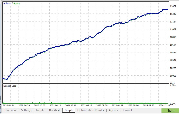
Test results on EURUSD/AUDUSD pair
This classic pair of instruments exhibits high historical correlation. Testing over the past 5 years has shown the following results:
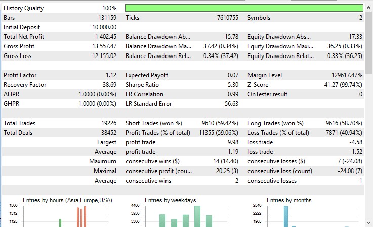
- Total profit: +14% to the initial deposit
- Maximum drawdown: 0.33%
- Percentage of profitable trades: 59%
- The average trade duration is 3 hours 42 minutes
- Sharpe Ratio: 5.3
The strategy has proven particularly efficient during periods of increased volatility, such as Brexit and the COVID-19 pandemic, when temporary deviations in correlation have created numerous trading opportunities.
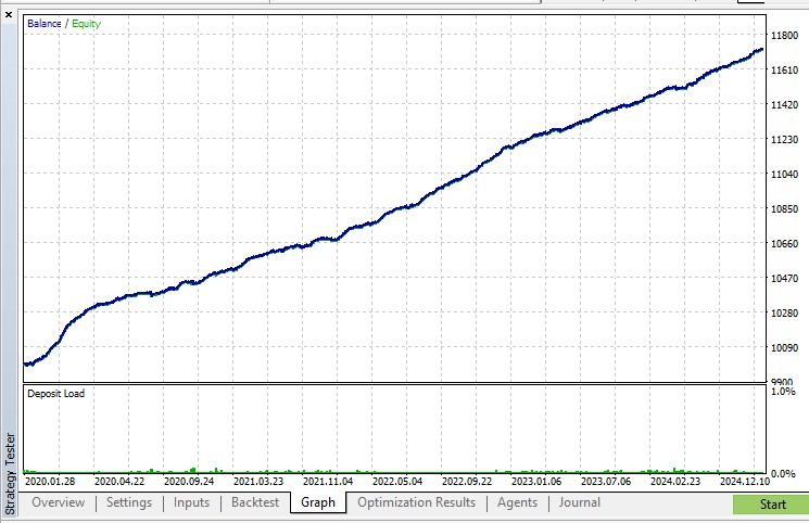
Results on AUDUSD/NZDUSD
The Australian and New Zealand dollar currency pairs also exhibit a high correlation due to the similar structure of their commodity-oriented economies. Test results:
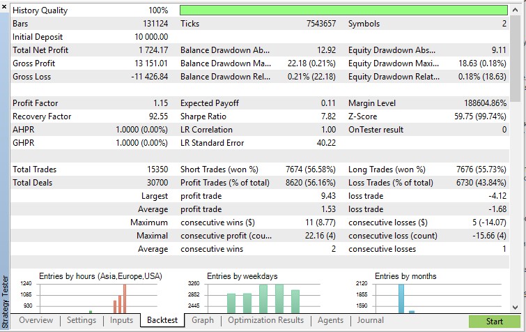
- Total profit: +17% to the initial deposit
- Maximum drawdown: 0.21%
- Percentage of profitable trades: 56%
- The average trade duration is 3 hours 26 minutes
- Sharpe Ratio: 7.82
An interesting feature of this pair is the shorter average trade duration, which is explained by the faster reversion to the mean of the correlation.
Setting parameters depending on the timeframe
The choice of the optimal timeframe depends on the trading time horizon. For medium-term trading (positions held from several days to several weeks), it is recommended to use a daily or 4-hour timeframe. For short-term trading (positions held from several hours to several days), an hourly or 15-minute timeframe is suitable.
When changing the timeframe, we need to adjust the parameters accordingly:
- On higher timeframes (D1, H4), the Z-score calculation period should be increased and entry/exit thresholds should be reduced.
- On lower timeframes (H1, M15), you should reduce the Z-score calculation period and increase entry/exit thresholds to filter out market noise.
Development prospects and further improvements
Although the current version of the algorithm already shows good results, there are several areas for further improvement.
Application of machine learning methods
One promising area is the integration of machine learning methods to predict the dynamics of correlation between instruments. Algorithms, such as LSTM (Long Short-Term Memory) neural networks, can effectively capture complex patterns in correlation relationships and predict their changes with high accuracy.
Extension to multi-currency portfolios
The current version of the algorithm works with a pair of currencies, but the concept can be expanded to a multi-currency portfolio, where correlations between several instruments are tracked simultaneously. This approach will allow us to more effectively utilize diversification and find trading opportunities across a wider range of market conditions.
Integration with fundamental analysis
Another promising direction is the integration of fundamental economic metrics into the decision-making algorithm. For example, taking into account differences in interest rates, inflation, and other macroeconomic indicators can help better predict long-term changes in the correlation relationships between currency pairs.
Conclusion
The presented pair trading algorithm with auto optimization demonstrates how relatively simple statistical principles can be transformed into an efficient trading system using modern algorithmic trading methods.
The key advantage of our approach is its adaptability: unlike systems with fixed parameters, our algorithm continuously adapts to changing market conditions, ensuring its long-term viability.
It is important to note that, despite the automation of the trading process, a deep understanding of the algorithm's operating principles and regular monitoring of its operation remain necessary conditions for the successful application of this strategy.
In the next article, we will explore further improvements to our algorithm, including the use of machine learning methods to predict correlation dynamics and parameter optimization using genetic algorithms.
Translated from Russian by MetaQuotes Ltd.
Original article: https://www.mql5.com/ru/articles/17800
Warning: All rights to these materials are reserved by MetaQuotes Ltd. Copying or reprinting of these materials in whole or in part is prohibited.
This article was written by a user of the site and reflects their personal views. MetaQuotes Ltd is not responsible for the accuracy of the information presented, nor for any consequences resulting from the use of the solutions, strategies or recommendations described.

- Free trading apps
- Over 8,000 signals for copying
- Economic news for exploring financial markets
You agree to website policy and terms of use
[T]he strategy in this article works best with Renko type chart
Renko charts are timeless, if you will. Even though each Renko brick still has a timestamp, the time scale of a custom Renko chart is not evenly incremented. Therefore, using Renko can potentially take the guesswork of manually selecting the best timeframe out of the trading process. Instead, you would be left to select the best brick size. Also, Renko inherently smooths out chart noise─every brick is the same size.
[W]hat are those above images about? What are you trying to tell us?
Although I can't read Chinese, I can read a pictograph. It appears that enabling "profit in pips for faster calculation" for this code is profitable in the Tester, while disabling it is unprofitable in the Tester.
Hello, Its an interesting strategy, I tried it on indices.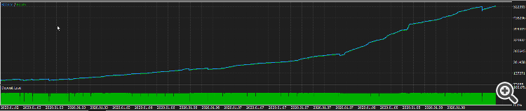
How to reduce the number of trades? Its taking too many until the Z score is below or above 2.