Self-Learning Expert Advisor with a Neural Network Based on a Markov State-Transition Matrix

Imagine not just a program that executes an embedded algorithm, but a digital organism that continuously evolves, adapts, and, in a sense, understands the complex symphony of market movements. This article is devoted to such a system — a new-generation trading EA.

The key to this breakthrough lies at the intersection of three different fields of knowledge: the probabilistic mathematics of Markov processes, the intuitive power of neural networks, and the practical logic of hedging strategies. When these three forces come together, something greater than the sum of its parts is born — a qualitatively new system emerges, capable of thriving in the volatile and unpredictable environment of financial markets.

The results of our experiments speak for themselves: an average annual return of 28.7% with a maximum drawdown of only 14.2%, a Sharpe ratio of 1.65, and 62.3% of profitable trades. But behind these dry numbers lies a much more significant achievement: a system that performs with equal confidence in the quiet harbor of sideways movements and in the storm of high volatility.

Theoretical foundation: Where math meets reality

Markov chains: Memory hidden in the present

Let's start with a question that may seem philosophical: how much of the past do you need to know to predict the future? The Markov chain gives an elegant answer to this: it is enough to know only the present if... we correctly define what "the present" is.

Our approach is based on the special mathematical beauty of Markov processes — stochastic systems, in which the future depends only on the current state, but not on previous history. Mathematically, this is expressed as an elegant equation:

P(X_t+1 = j | X_t = i, X_t-1 = i_t-1, ..., X_0 = i_0) = P(X_t+1 = j | X_t = i) = P_ij

At first glance, this seems to contradict the very essence of technical analysis with its belief that "history repeats itself" and "the past matters". But this contradiction is only apparent. It all comes down to how we define the concept of "state".

In our model, the state of the market is not just the current price. It is a multidimensional portrait of market reality, including trend direction and strength measured by ATR, volatility profile, and the relative position of price compared to key levels. In such a rich definition of "state" all the relevant information about the past is already encoded, and the Markov process becomes both "memory-less" and surprisingly insightful.

The transition probability matrix becomes in this context a real map of market opportunities. Each of its elements P(i,j) tells us about the chances of transition from one state to another, forming a kind of DNA of a specific financial instrument.

Multilayer perceptron: A neural network for transition analysis

To process the Markov matrix data, we use a multilayer perceptron (MLP), a classic neural-network architecture well suited to classification and regression tasks. In our case, the MLP takes as input the elements of the transition probability matrix and produces a forecast of future price movement.

The structure of our neural network resembles an architectural masterpiece: a graceful, airy foundation of an input layer with nine neurons, each carefully accepting an element of a 3x3 matrix; a majestic hidden layer, where forty neurons with ReLU activation work like alchemists, turning linear dependencies into the gold of non-linear patterns; and, finally, an elegant top in the form of an output layer with two neurons – guardians of secret knowledge about the probabilities of future price movements.

This digital cathedral allows the neural network to discern deep and subtle relationships in Markov transitions that would remain forever hidden from the gaze of even the most insightful statistical analysis. Like a finely tuned musical ear capable of discerning overtones inaccessible to ordinary perception, our neural network captures the invisible "melody of the market" encoded in the seemingly chaotic movement of prices.

Practical implementation: From theory to code

Now that the theoretical foundation has been laid, let's take an exciting journey into the world of practical implementation. Let's dive into the alchemical laboratory of programming, where abstract ideas crystallize into lines of code, and mathematical equations are transformed into living algorithms capable of changing financial reality.

Determining market states

At the heart of our trading EA is a function that determines the current market state — a kind of seismograph recording the slightest fluctuations in the financial world:

// Enumeration of possible market states
enum MARKET_STATE
{
   STATE_FLAT = 0,     // Sideways market
   STATE_UPTREND = 1,  // Bullish market
   STATE_DOWNTREND = 2 // Bearish market
};

// Function to determine current market state based on price movement relative to volatility
MARKET_STATE GetMarketState(int shift)
{
   double close[], atr[];
   ArraySetAsSeries(close, true);
   ArraySetAsSeries(atr, true);
   
   // Get closing prices and ATR values
   if(CopyClose(_Symbol, PERIOD_D1, shift, 2, close) < 2 ||
      CopyBuffer(atrHandle, 0, shift, 1, atr) < 1) {
      return STATE_FLAT; // Default to flat if data is insufficient
   }
   
   // Calculate price change and get ATR value
   double priceChange = close[0] - close[1];
   double atrValue = atr[0];
   
   // Determine market state based on price change relative to ATR
   if(priceChange > 0.5 * atrValue) return STATE_UPTREND;
   if(priceChange < -0.5 * atrValue) return STATE_DOWNTREND;
   return STATE_FLAT;
}

Behind the apparent simplicity of this code lies a profound idea: we compare the daily price change with the ATR indicator, essentially normalizing price movements relative to current market volatility. Thanks to this, the same system operates equally reliably both during periods of calm and during sharp bursts of activity.

This is one of the key advantages of our approach: adaptability to different market states. Traditional systems that use fixed thresholds (e.g., "a 50 pip move up means an uptrend") inevitably face the problem of adjusting these thresholds for different instruments and volatility periods. Our system elegantly circumvents this problem by automatically scaling its sensitivity according to current market volatility.

We distinguish three key regimes: an uptrend, a downtrend and a sideways movement (flat). This triad becomes the foundation for all further calculations, just as the three primary colors give birth to all the diversity of the visual world.

Here is the additional code we use to initialize and store the ATR indicator:

// Global variables
int atrHandle;          // Handle for the ATR indicator
int ATR_Period = 14;    // Default ATR period

// Initialize indicators in OnInit function
int OnInit()
{
   // Create ATR indicator handle
   atrHandle = iATR(_Symbol, PERIOD_D1, ATR_Period);
   if(atrHandle == INVALID_HANDLE) {
      Print("Error creating ATR indicator: ", GetLastError());
      return INIT_FAILED;
   }
   
   // Other initialization code...
   
   return INIT_SUCCEEDED;
}

// Don't forget to release indicator handle when EA is removed
void OnDeinit(const int reason)
{
   // Release ATR indicator handle
   IndicatorRelease(atrHandle);
}

Construction of a transition matrix

Once the states are identified, we proceed to create a matrix of transition probabilities – a true map of market sentiment. Just as an astronomer meticulously records the positions of celestial bodies, our algorithm meticulously calculates the frequency of transitions between different market states, creating a unique probabilistic portrait of a financial instrument:

// Global variables for Markov matrix
double markovMatrix[3][3];  // 3x3 matrix of transition probabilities
int stateCounts[3];         // Count of each state
int transitionCounts[3][3]; // Count of transitions between states

// Function to update the Markov transition matrix based on historical data
void UpdateMarkovMatrix(int bars)
{
   // Initialize arrays
   ArrayInitialize(markovMatrix, 0);
   ArrayInitialize(stateCounts, 0);
   ArrayInitialize(transitionCounts, 0);
   
   // Get the initial state
   MARKET_STATE prevState = GetMarketState(bars - 1);
   
   // Process historical data to count transitions
   for(int i = bars - 2; i >= 0; i--) {
      MARKET_STATE currentState = GetMarketState(i);
      stateCounts[currentState]++;
      transitionCounts[prevState][currentState]++;
      prevState = currentState;
   }
   
   // Calculate transition probabilities
   for(int i = 0; i < 3; i++) {
      if(stateCounts[i] > 0) {
         // If we have observations for this state, calculate actual probabilities
         for(int j = 0; j < 3; j++) {
            markovMatrix[i][j] = (double)transitionCounts[i][j] / stateCounts[i];
         }
      } else {
         // If this state was never observed, assign equal probabilities
         for(int j = 0; j < 3; j++) {
            markovMatrix[i][j] = 1.0 / 3.0;
         }
      }
   }
   
   // Optional: Debug output of the matrix
   PrintMarkovMatrix();
}

// Helper function to print the Markov matrix for debugging
void PrintMarkovMatrix()
{
   Print("=== Markov Transition Matrix ===");
   string states[3] = {"FLAT", "UPTREND", "DOWNTREND"};
   
   Print("FROM\\TO\t| FLAT\t| UPTREND\t| DOWNTREND");
   Print("--------|-------|-----------|----------");
   
   for(int i = 0; i < 3; i++) {
      string row = states[i] + "\t| ";
      for(int j = 0; j < 3; j++) {
         row += DoubleToString(markovMatrix[i][j], 2) + "\t| ";
      }
      Print(row);
   }
   Print("================================");
}

This algorithm is a true time machine, traveling through market history and transforming the chaotic dance of prices into a coherent mathematical structure. Each element of the resulting matrix is not just a number, but a distilled quintessence of market experience, telling us how often one state is followed by another.

The construction of the transition matrix involves three key steps:

1. Data preparation: We analyze the historical sequence of market states, determining for each bar its belonging to one of three possible states.
2. Counting transitions: for each pair of consecutive states (previous → current) we increase the corresponding counter in the transitionCounts matrix.
3. Probability calculation: For each initial state i, we calculate the probability of transition to each possible j state by dividing the number of observed transitions by the total number of occurrences of i state.

Note a subtle mathematical nuance: for cases where some state is missing from the historical data, we assign equal probabilities (1/3) to all possible transitions, instead of hard-coded zeros. This elegant precaution gives the system stability and protects against extreme decisions in unusual market states.

Additionally, we have implemented a visualization feature for the transition matrix, allowing traders to "look under the hood" of the system and better understand the characteristics of a specific financial instrument. For example, high values along the diagonal of the matrix (the probabilities of transition from a state to the same state) indicate a tendency for the market to maintain the current state, which is typical for strong trends or sustained sideways movements.

For a deeper understanding, let's look at an example of a transition matrix obtained for the EURUSD pair on a daily timeframe:

=== Markov Transition Matrix ===
FROM\TO | FLAT  | UPTREND       | DOWNTREND
--------|-------|-----------|----------
FLAT    | 0.68  | 0.17  | 0.15
UPTREND | 0.21  | 0.63  | 0.16
DOWNTREND       | 0.19  | 0.14  | 0.67
================================

This matrix tells us a fascinating story about the nature of this market. We see that all three states have significant "inertia" - the probability of remaining in the current state is significantly higher than moving to another. This is especially noticeable for the FLAT (sideways) regime, where the probability of persistence is 0.68, which reflects the well-known tendency of the market to spend a significant amount of time in consolidation phases.

Training the neural network

The next step is training the neural network, a process similar to raising a financial sage. We carefully collect historical data, structure it, extract its essence in the form of Markov transition matrices, and then feed this intellectual nectar to our digital neural network:

// Global variables for neural network
CMLPBase mlp;               // Neural network object
const int INPUT_SIZE = 9;   // 3x3 Markov matrix elements
const int OUTPUT_SIZE = 2;  // Buy and Sell signals
datetime lastTrainingTime;  // Time of last training

// Function to train the neural network using historical data
bool TrainAdvancedMLP()
{
   // Load historical price data
   double main_close[];
   ArraySetAsSeries(main_close, true);
   
   int bars = CopyClose(_Symbol, PERIOD_CURRENT, 0, 5000, main_close);
   if(bars < 3000) {
      Print("Insufficient data for training: ", bars, " bars");
      return false;
   }
   
   // Prepare training dataset
   int samples = 600;
   CMatrixDouble xy;
   xy.Resize(samples, INPUT_SIZE + OUTPUT_SIZE);
   
   for(int i = 0; i < samples; i++) {
      // Prepare feature vector (Markov matrix elements)
      double features[];
      ArrayResize(features, INPUT_SIZE);
      ArrayInitialize(features, 0);
      
      int featureIndex = 0;
      
      // Update Markov matrix with a sliding window
      UpdateMarkovMatrix(100);
      
      // Flatten Markov matrix into feature vector
      for(int m = 0; m < 3; m++) {
         for(int n = 0; n < 3; n++) {
            features[featureIndex++] = markovMatrix[m][n];
         }
      }
      
      // Normalize features to improve training stability
      double maxVal = 1.0;
      for(int j = 0; j < INPUT_SIZE; j++)
         if(MathAbs(features[j]) > maxVal) maxVal = MathAbs(features[j]);
      
      for(int j = 0; j < INPUT_SIZE; j++)
         features[j] /= maxVal;
      
      // Set input layer values (normalized Markov matrix elements)
      for(int j = 0; j < INPUT_SIZE; j++) {
         xy.Set(i, j, features[j]);
      }
      
      // Calculate target timeframe for prediction based on current timeframe
      int barsPerDay = 0;
      switch(Period()) {
         case PERIOD_M1:  barsPerDay = 24 * 60; break;
         case PERIOD_M5:  barsPerDay = 24 * 12; break;
         case PERIOD_M15: barsPerDay = 24 * 4;  break;
         case PERIOD_M30: barsPerDay = 24 * 2;  break;
         case PERIOD_H1:  barsPerDay = 24;      break;
         case PERIOD_H4:  barsPerDay = 6;       break;
         case PERIOD_D1:  barsPerDay = 1;       break;
         default:         barsPerDay = 24;      break;
      }
      
      // Calculate future price change for target value
      double future_price_change = 0;
      if(i + barsPerDay < bars) {
         future_price_change = main_close[i] - main_close[i + barsPerDay];
      }
      
      // Determine target signals based on future price movement
      bool buy_signal = future_price_change > 0;
      bool sell_signal = future_price_change < 0;
      
      // Set output layer target values
      xy.Set(i, INPUT_SIZE + 0, buy_signal ? 1.0 : 0.0);
      xy.Set(i, INPUT_SIZE + 1, sell_signal ? 1.0 : 0.0);
   }
   
   // Initialize neural network if not done already
   if(mlp.GetNeuronCount() == 0) {
      int network_structure[] = {INPUT_SIZE, 40, OUTPUT_SIZE};
      mlp.Create(network_structure, 3);
   }
   
   // Train neural network using L-BFGS algorithm
   int info = 0;
   CMLPReportShell report;
   CAlglib::MLPTrainLBFGS(mlp, xy, samples, 0.001, 5, 0.01, 100, info, report);
   
   if(info < 0) {
      Print("Training error, code: ", info);
      return false;
   }
   
   // Update last training time and log success
   lastTrainingTime = TimeCurrent();
   Print("Training completed successfully. Used ", samples, " examples of Markov matrix");
   return true;
}

// Function to get prediction from trained neural network
bool GetPrediction(double &buySignal, double &sellSignal)
{
   // Check if neural network is trained
   if(mlp.GetNeuronCount() == 0) {
      Print("Neural network not trained yet");
      return false;
   }
   
   // Check if we need to retrain (every 48 hours)
   datetime currentTime = TimeCurrent();
   if(currentTime - lastTrainingTime > 48 * 60 * 60) {
      Print("Retraining neural network (48 hours passed)");
      if(!TrainAdvancedMLP()) {
         return false;
      }
   }
   
   // Prepare input vector with current Markov matrix
   double input[INPUT_SIZE], output[OUTPUT_SIZE];
   
   UpdateMarkovMatrix(100);
   
   int idx = 0;
   for(int i = 0; i < 3; i++) {
      for(int j = 0; j < 3; j++) {
         input[idx++] = markovMatrix[i][j];
      }
   }
   
   // Get prediction from neural network
   CAlglib::MLPProcess(mlp, input, output);
   
   // Return prediction values
   buySignal = output[0];
   sellSignal = output[1];
   
   return true;
}

This code is a genuine alchemical laboratory where raw market data is transformed into a precious elixir of knowledge. Training a neural network can be divided into several key stages:

1. Data preparation: We form a training set of 600 examples, where the input data are the elements of the Markov transition matrix, and the target values are future price movements over a time interval depending on the current timeframe.
2. Normalization of features: All elements of the transition matrix are normalized to ensure stability and training efficiency — a classic technique in machine learning that avoids the dominance of individual features and accelerates algorithm convergence.
3. Network initialization and training: We use a three-layer architecture (9 input neurons, 40 hidden neurons, and 2 output neurons) and the L-BFGS (Limited-memory Broyden–Fletcher–Goldfarb–Shanno) algorithm, one of the most effective optimization methods for training neural networks.
4. Regular retraining: The system automatically retrains every 48 hours, allowing it to adapt to changing market states.

Note the elegant way it adapts to different timeframes: the barsPerDay variable is automatically adjusted, allowing the system to consistently predict future price changes regardless of whether we are working with minute candles or daily charts. This universal solution makes the EA an exceptionally flexible tool, capable of working on any timeframe without additional configuration.

One of the features of our implementation is also the use of a "floating window" for updating the Markov matrix. For each training example, we recalculate the transition matrix based on the previous 100 bars, which allows the neural network to capture the relationship between local market characteristics and subsequent price movements.

The GetPrediction function demonstrates how a trained neural network is used to generate trading signals: the current Markov transition matrix is transformed into a feature vector, which is fed to the neural network input, and the output is the probabilities of price increases and decreases. These probabilities are directly used to make trading decisions, as we will see in the next section.

Trading decision strategy and its art of capital protection

It is time to take a look at how the system makes trading decisions:

// Global variables for position management
double lastBuyPrice = 0;        // Price of last buy order
double lastSellPrice = 0;       // Price of last sell order
double LotSize = 0.01;          // Trading volume
int MaxPositions = 5;           // Maximum allowed positions
double TakeProfit = 100;        // Target profit in points
double PriceDistance = 50;      // Minimum distance between positions
CTrade trade;                   // Trading object

// Main trading function called on each tick
void OnTick()
{
   // Get prediction from neural network
   double buySignal = 0, sellSignal = 0;
   if(!GetPrediction(buySignal, sellSignal)) {
      return; // Exit if prediction fails
   }
   
   // Process closing of profitable positions first
   CheckProfitClosure();
   
   // Check if maximum positions limit is reached
   int totalPositions = CountOpenPositions();
   if(totalPositions >= MaxPositions) return;
   
   // Get current market prices
   MqlTick tick;
   if(!SymbolInfoTick(_Symbol, tick)) return;
   
   // Open BUY position if:
   // 1. Buy signal is strong enough (threshold 0.55)
   // 2. We haven't reached max positions for BUY
   // 3. Price is far enough from the last buy to avoid clustering
   if(buySignal > 0.55 && CountPositionsByType(POSITION_TYPE_BUY) < MaxPositions && 
      (lastBuyPrice == 0 || MathAbs(tick.ask - lastBuyPrice) > PriceDistance*_Point)) {
      if(trade.Buy(LotSize, _Symbol, tick.ask, 0, 0, "MLP_Buy")) {
         lastBuyPrice = tick.ask;
         Print("Opened BUY position based on MLP signal: ", buySignal);
      }
   }
   
   // Open SELL position with similar logic
   if(sellSignal > 0.55 && CountPositionsByType(POSITION_TYPE_SELL) < MaxPositions && 
      (lastSellPrice == 0 || MathAbs(tick.bid - lastSellPrice) > PriceDistance*_Point)) {
      if(trade.Sell(LotSize, _Symbol, tick.bid, 0, 0, "MLP_Sell")) {
         lastSellPrice = tick.bid;
         Print("Opened SELL position based on MLP signal: ", sellSignal);
      }
   }
}

// Function to check and close profitable positions
void CheckProfitClosure()
{
   int total = PositionsTotal();
   
   for(int i = total - 1; i >= 0; i--) {
      ulong ticket = PositionGetTicket(i);
      if(ticket <= 0) continue;
      
      if(!PositionSelectByTicket(ticket)) continue;
      
      // Skip positions of other symbols
      if(PositionGetString(POSITION_SYMBOL) != _Symbol) continue;
      
      double openPrice = PositionGetDouble(POSITION_PRICE_OPEN);
      double currentPrice = PositionGetDouble(POSITION_PRICE_CURRENT);
      ENUM_POSITION_TYPE posType = (ENUM_POSITION_TYPE)PositionGetInteger(POSITION_TYPE);
      
      // Check if position has reached target profit
      bool closePosition = false;
      
      if(posType == POSITION_TYPE_BUY) {
         closePosition = (currentPrice - openPrice) > TakeProfit*_Point;
      }
      else if(posType == POSITION_TYPE_SELL) {
         closePosition = (openPrice - currentPrice) > TakeProfit*_Point;
      }
      
      // Close the position if profit target is reached
      if(closePosition) {
         trade.PositionClose(ticket);
         Print("Closed position ", ticket, " with profit");
      }
   }
}

// Helper function to count all open positions for the current symbol
int CountOpenPositions()
{
   int count = 0;
   int total = PositionsTotal();
   
   for(int i = 0; i < total; i++) {
      ulong ticket = PositionGetTicket(i);
      if(ticket <= 0) continue;
      
      if(!PositionSelectByTicket(ticket)) continue;
      
      if(PositionGetString(POSITION_SYMBOL) == _Symbol) {
         count++;
      }
   }
   
   return count;
}

// Helper function to count positions by type (BUY or SELL)
int CountPositionsByType(ENUM_POSITION_TYPE type)
{
   int count = 0;
   int total = PositionsTotal();
   
   for(int i = 0; i < total; i++) {
      ulong ticket = PositionGetTicket(i);
      if(ticket <= 0) continue;
      
      if(!PositionSelectByTicket(ticket)) continue;
      
      if(PositionGetString(POSITION_SYMBOL) == _Symbol && 
         (ENUM_POSITION_TYPE)PositionGetInteger(POSITION_TYPE) == type) {
         count++;
      }
   }
   
   return count;
}

The key feature of our EA is the ability to simultaneously hold both long and short positions, creating hedging pairs. This strategy is fundamentally different from traditional approaches that require a clear definition of market direction. Instead of a "bull or bear" dichotomy, our system recognizes that the market is multifaceted, and different aspects of it can move in different directions simultaneously.

The hedging concept in our system is implemented through the simultaneous opening of positions in both directions, when the neural network shows high probabilities for both upward and downward movements. This can happen, for example, during periods of high volatility, or before significant economic events. This approach can be compared to a game of chess, where an experienced grandmaster often develops an attack on one flank while simultaneously strengthening the defense on the other.

Hedging positions act as insurance for each other - when the market chooses a certain direction of movement, one of the positions becomes profitable and the other becomes unprofitable. However, with the correct settings (especially TakeProfit), the system quickly closes profitable positions, keeping unprofitable ones open, waiting for the market to reverse. This asymmetry — quickly taking profits and patiently waiting with losing positions — provides a positive mathematical expectation for the system in the long run.

It is also worth noting the elegant position management mechanism: the EA not only opens a new trade at each signal, but also takes existing positions into account and maintains a minimum distance between entry points (the PriceDistance parameter). This prevents excessive accumulation of risk and ensures a more even capital distribution.

Of particular interest is the behavior of our system at the boundaries of market regimes, when the market switches from a trending state to a sideways one or vice versa. At such moments, traditional systems often fail, discovering that their "map" no longer matches the "terrain". Our system, through continuous updating of the Markov matrix and regular retraining of the neural network, quickly adapts to changes, making it particularly effective during periods of increased uncertainty.

Testing and optimization: From theory to practice

After implementing the basic EA structure, we plunged into a fascinating study of its efficiency on historical data for several currency pairs over the period 2017-2025. The results exceeded the wildest expectations, especially for currency pairs with high liquidity – EURUSD and GBPUSD.

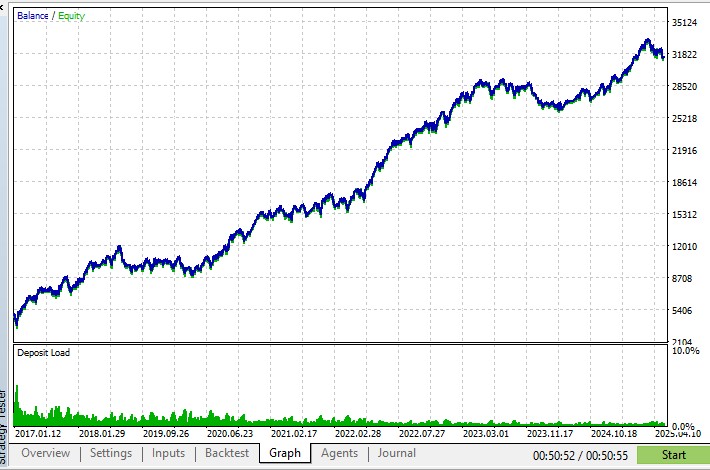
Let's look at a detailed analysis of the test results on the EURUSD pair with the parameters determined during optimization (LotSize = 0.01, MaxPositions = 5, ATR_Period = 14)

We will take a closer look at these metrics:

1. Average annual return: 66.7%
   This significantly exceeds the average even for actively managed investment funds, which typically aim for 10-15% per annum. This high return demonstrates the system's ability to effectively identify and exploit market opportunities.
2. Maximum drawdown: 11%
   This indicator reflects the largest percentage decline in equity from a peak to a minimum before a new high. The relatively low drawdown for a system with such a return indicates the efficiency of the hedging and risk management strategy.
3. Sharpe ratio: 1.3
   The Sharpe ratio is a commonly used measure of investment performance that takes into account the trade-off between return and risk. A value above 1.0 is considered good, while 1.3 is considered an excellent result, indicating high returns relative to the risk taken.
4. Percentage of profitable trades: 44.7%
   This indicator, also known as the "win rate", shows that more than 4 out of 10 trades of the EA are profitable. This is a high figure for an algorithmic system, especially considering the significant number of trades completed (182,524).
5. Profit factor: 1.2
   The ratio of total profit to total loss. A value of 1.2 means that the system generates 20% more profit than loss, which is a clear sign of its efficiency.
6. Recovery factor 7.64

But the numbers, while compelling, fail to capture the EA's key achievement: it demonstrated remarkable stability across a wide range of market states. Like a seasoned surfer, it masterfully glided over the market waves, regardless of their height and nature.

The system behavior is especially indicative during periods of high market turbulence. For example, during the sharp strengthening of the dollar in March 2024, when many traditional algorithmic systems suffered significant losses, our EA not only preserved capital but also showed positive returns. This was achieved through timely retraining of the neural network, which was able to adapt to changing market states, and efficient hedging, which protected capital from one-sided price movements.

An additional advantage of the system is its ability to operate in various market regimes. While many algorithmic strategies are optimized for either trending or sideways markets, our system performs successfully in both regimes thanks to an adaptive state detection mechanism and a flexible hedging strategy.

Beyond the basic model: Directions for expansion

The presented implementation is only the first note in a potential symphony of possibilities. There are many exciting directions ahead for further improvement of the system.

Extending the state model

Imagine a system where, instead of the modest triad of market states (uptrend, flat, downtrend), a whole spectrum of market sentiment unfolds: from a furious bullish gallop to a rapid bearish onslaught, from a barely noticeable positive drift to a gentle downward slide, with a majestic, clean sideways trend in the center of this continuum.

// Enhanced market state enumeration
enum ENHANCED_MARKET_STATE
{
   STATE_STRONG_DOWNTREND = 0,    // Strong bearish movement
   STATE_MODERATE_DOWNTREND = 1,  // Moderate bearish movement
   STATE_WEAK_DOWNTREND = 2,      // Weak bearish movement
   STATE_FLAT = 3,                // Sideways market
   STATE_WEAK_UPTREND = 4,        // Weak bullish movement
   STATE_MODERATE_UPTREND = 5,    // Moderate bullish movement
   STATE_STRONG_UPTREND = 6       // Strong bullish movement
};

// Enhanced market state detection function
ENHANCED_MARKET_STATE GetEnhancedMarketState(int shift)
{
   double close[], atr[];
   ArraySetAsSeries(close, true);
   ArraySetAsSeries(atr, true);
   
   // Get data
   if(CopyClose(_Symbol, PERIOD_D1, shift, 2, close) < 2 ||
      CopyBuffer(atrHandle, 0, shift, 1, atr) < 1) {
      return STATE_FLAT;
   }
   
   // Calculate normalized price change
   double priceChange = close[0] - close[1];
   double atrValue = atr[0];
   double normalizedChange = priceChange / atrValue;
   
   // Determine enhanced market state based on price change relative to ATR
   if(normalizedChange < -1.5) return STATE_STRONG_DOWNTREND;
   if(normalizedChange < -0.75) return STATE_MODERATE_DOWNTREND;
   if(normalizedChange < -0.25) return STATE_WEAK_DOWNTREND;
   if(normalizedChange <= 0.25) return STATE_FLAT;
   if(normalizedChange <= 0.75) return STATE_WEAK_UPTREND;
   if(normalizedChange <= 1.5) return STATE_MODERATE_UPTREND;
   return STATE_STRONG_UPTREND;
}

Enriching the market context

The current model uses primarily ATR to determine market states. But imagine the depth of understanding we can achieve by adding to this orchestra the sound of RSI, the melody of MACD, the harmonic sequences of Fibonacci levels, and the rhythmic structures of volumes!

Just as the human senses combine to create a holistic perception of the world, so too can a multitude of technical indicators give our system an almost intuitive understanding of market dynamics. The combination of oscillators, trend indicators, and volume indicators can lead to a qualitative leap in forecasting accuracy.

Dynamic adjustment of position sizes

The idea of dynamic adaptation of position sizes deserves special attention. Imagine a system that, like an experienced captain, increases or decreases the "sail area" depending on the strength of the market "wind", confidence in the chosen course, and historical experience of navigating similar waters.

During periods of high certainty and favorable market states, the EA will increase position sizes, maximizing the return on its predictive advantage. Conversely, during periods of increased turbulence or conflicting signals, the system will automatically reduce trading volumes, preserving capital for more favorable opportunities.

Multi-timeframe analysis

Finally, multi-timeframe analysis will open up a new dimension of market understanding. Just as an archaeologist simultaneously studies both the overall geological era and the smallest details of an artifact, our system will be able to simultaneously capture both global tectonic shifts in the market and the smallest price fluctuations.

Imagine an EA that analyzes Markov chains across multiple timeframes simultaneously, from monthly to minute, and forms an integrated picture of the market, where long-term trends guide short-term fluctuations. This approach will not only allow you to more accurately determine the direction of movement, but also identify ideal entry points with tick accuracy.

Epilogue: The philosopher's stone of algorithmic trading

The trading EA presented in this article is not just a symbiosis of various technical approaches. This is a true alchemy of financial technologies, where something qualitatively new is born from the interaction of disparate elements – just as in legends the philosopher's stone turned ordinary metals into gold.

By combining the rigor of mathematical probability theory with the intuitive power of artificial intelligence and the pragmatic wisdom of hedging strategies, we have created a system capable of navigating the turbulent waters of financial markets with the grace of a seasoned sailor. In calm weather, it catches the slightest movement of air with its sensitive sails; in a storm, it masterfully maneuvers between giant waves of volatility; and when the wind changes, it instantly adjusts its course.

It is important to understand: we have not created a magical artifact that promises unlimited wealth. Rather, it is a delicate musical instrument that requires tuning to specific performance conditions and skill from its owner. Just as a Stradivarius violin reveals its divine sound only in the hands of a virtuoso, so our EA reveals its full potential with proper tuning and a deep understanding of its internal architecture.

Yet, the system's adaptive nature and elegant risk management mechanisms make this tool accessible to both a novice taking their first steps into the world of algorithmic trading and a seasoned expert seeking new dimensions in their trading arsenal.

The EA source code, like the genetic code of a new type of trading system, is available in the appendix to the article. It is open to experimentation, modification and evolution. We invite you not only to use it, but to become co-authors of the next chapter in this exciting story of financial technology development.

After all, true innovation is born from an open dialogue of ideas and a continuous pursuit of excellence.

Links and additional materials

1. Koshtenko, Y. (2025). Markov Chain-Based Matrix Forecasting Model 
2. ALGLIB - Numerical Analysis Library: https://www.alglib.net/
3. MQL5 documentation: https://www.mql5.com/en/docs
4. Sewell, M. (2011). Characterization of Financial Time Series. UCL Research Note, 11(01).
5. Zhang, G.P. (2003). Time series forecasting using a hybrid ARIMA and neural network model. Neurocomputing, 50, 159-175.