MQL5 Wizard Techniques you should know (Part 58): Reinforcement Learning (DDPG) with Moving Average and Stochastic Oscillator Patterns

Introduction

From our last article, we tested 10 signal patterns from our 2 indicators (MA & Stochastic Oscillator).  Seven were able to forward-walk based on a 1-year test window. However, of these, only 2 did so by placing both long and short trades. This was down to our small test-window, which is why readers are urged to test this on more history before taking it any further. 

We are following a thesis here where the three main modes of machine learning can be used together, each in its own ‘phase’. These modes, to recap, are supervised-learning (SL), reinforcement-learning (RL), and inference-learning (IL). We dwelt on SL in the last article, where combined patterns of the moving average and stochastic oscillator were normalized to a binary vector of features. This was then fed into a simple neural network that we trained on the pair EUR USD for the year 2023 and subsequently performed forward tests for the year 2024. 

Since our approach is based on the thesis RL can be used to train models while in use, we want to demonstrate this in this article by using our earlier results & network from SL. RL, we are positing, is a form of back propagation when in deployment that carefully fine-tunes our buy-sell decisions so that they are not solely based on projected changes in price alone as was the case in the SL model. 

This ‘fine-tuning’ as we have seen in past RL articles, marries exploration and exploitation. So, in doing so, our policy network would from training in a live market environment determine which states should result in buy or sell actions. There could be cases where a bullish state would not necessarily mean a buying opportunity, and vice versa. This means that our RL model acts as an extra filter to the decisions made by the SL model. The states from our SL model were using single-dim continuous values, and this will be very similar to the action space we will be using.

DDPG

We have already considered a number of different RL algorithms, and for this article we are looking at Deep Deterministic Policy Gradient (DDPG). This particular algorithm, a bit like DQN that we considered in an earlier article, serves to make forecasts in continuous action spaces. Recall for most of the algorithms we have recently looked at, they were classifiers, looking to output probability distributions on whether the next course of action should be buy, sell, or hold (for example). 

This one is not a classifier but a regressor. We define an action space as a floating point value in the range 0.0 to 1.0. This approach can be used to calibrate a lot more options than simply:

• buying (anything above 0.5);
• selling (anything below 0.5);
• or holding (anything close to 0.5)

This could be achieved by introducing pending order types or even position sizing. These measures are left to the reader to explore as we will be sticking to the bare-bones implementation where 0.5 serves as a key threshold. 

In principle, DDPG uses neural networks to approximate Q-values (rewards from actions) and directly optimizes the policy (network that choose the next best action  when presented with environment-states); instead of just estimating Q-Values. Unlike DQN that can also be used for discrete/ classification actions like left or right, DDPG is purely for continuous action spaces. (Think steering angles or motor torques when, say, training robotics). How does it work?

Primarily, two neural networks are used. 

• One is the Actor network, whose role is to decide the best action for a given environment-state. 
• The other is the critic network, whose purpose is to evaluate how good the action selected by the actor is through estimating the potential rewards that can be reaped for carrying out that action. 

This estimate is also referred to as the Q-Value. Also, important within DDPG is the experience replay buffer. This stores past-experiences (a collective term to represent states, actions, rewards, and next-states) in a buffer. Random samples from this buffer are used to train the networks and reduce correlation between updates.

Besides the 2 mentioned networks above, their equivalent copies that are referred to as ‘targets’ are also engaged. These separate copies of the actor and critic networks get their weights updated at a slower pace, and this it is argued helps stabilize the training process by providing consistent targets. Finally, exploration, a key feature in reinforcement-learning, is taken a step further in DDPG by introducing a noise component to the actions via algorithms, most common of which is the Ornstein-Uhlenbeck noise.

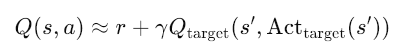
Training DDPG essentially covers 3 things. Firstly it involves improving the actor-network where the critic network guides the actor-network in defining which action is good/bad so that the actor network better adjusts its weight in picking actions that maximize rewards. Secondly, improving the critic-network where it learns to better estimate rewards/Q-Values using Bellman updates as laid out in the equation below:

Where:

• Q(s,a): The predicted Q-value (critic's estimate) for taking action a in state s.

• r: Immediate reward received after taking action a in state s.

• γ: Discount factor (0≤γ<1), which determines how much future-rewards are valued (closer to 0 = short-term focus, closer to 1 = long-term focus).

• s′: Next state observed after taking action a in state s.

• Qtarget(s′,⋅): Target Q-network's estimate of the Q-value for the next state s′(used to stabilize training).

• Actortarget(s′): Target actor's recommended action for the next state s′(deterministic policy).

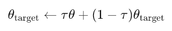
Finally, there are soft updates for the actor-target and critic-target, where updates are performed slowly to match the main networks in line with the following equation:

Where:

• θtarget: Parameters (weights) of the target network (either actor or critic).
• θ: Parameters of the main (online) network (either actor or critic).
• τ: Soft update rate (0≪τ≪1, e.g., 0.001). Controls how slowly the target networks are updated.
• Small τ = target networks change very slowly (more stable training).
• Large τ = target networks update faster (less stable but may adapt quicker).

Why DDPG? It is popular because it works well in high-dimensional, continuous action spaces, and it combines the stability of Q-Learning with the flexibility of policy-gradients. As shown in the robotics continuous action space example above, it is very popular in robotics, physics-based control and other similar complex tasks. This does not mean we cannot use it in financial time series, though, and that is what we will explore. 

We are implementing most of our code in Python 3.10 because of the efficiencies offered when training very deep networks. But in this field one learns something new every so often. In my case, it was that Python is actually able to pull off such fast computations in training networks (PyTorch & TensorFlow) thanks to anchor code and classes in C/C++ as well as CUDA. Now MQL5 is very similar to C and implementing OpenCL has been supported for some time. I think what this means is we simply lack a basic multiplication matrix code library (partly in OpenCL) to get similar performance in MQL5? This is something that might be worth exploring.

Replay Buffer

The replay buffer is a very important component in DDPG and other off-policy reinforcement learning algorithms. It mainly used to break temporal-correlations between consecutive samples, enable experience re-use so that learning can be more efficient,  provide a diverse set of transitions for stable training, and store past experiences (state, action, reward, next-state, done tuples) for use in the training/ network weight update process.

Its core implementation primarily starts with its initialization function:

def __init__(self, capacity):

    self.buffer = deque(maxlen=capacity)

We are using collections.deque with a fixed maximum capacity and automatically discarding old experiences when full via a First-In-First-Out behavior. It is very simple and memory efficient. Next is the push-operation, where the buffer stores complete transition tuples, and handles both successful and terminal transitions (by using the done flag). It provides a minimal overhead when adding new experiences.

def push(self, state, action, reward, next_state, done):

    self.buffer.append((state, action, reward, next_state, done))

The used sampling mechanism is a random uniform sampling that is very important for breaking correlations. It is efficient in that it uses batch processing via zip(*batch) which helps in separating the environment components. It returns all necessary components for Q-learning update.

def sample(self, batch_size):

    batch = random.sample(self.buffer, batch_size)

    states, actions, rewards, next_states, dones = zip(*batch)

Next in the replay buffer class is the tensor conversion and device handling for each of the environment components. These, as already shown above, are states, actions, rewards, next-states, and dones. The conversion is very robust. It handles both NumPy arrays and PyTorch tensors as input. This ensures tensors (which can be taken as arrays with gradient information attached) are detached from the computation graphs.

We move the data to the CPU to avoid device conflicts. We perform an explicit conversion to Float Tensor (float-32) that is a common prerequisite for neural networks. This data type that is smaller than the double often used in MQL5 is significantly more compute efficient. Finally, thanks to PyTorch (unlike TensorFlow), we can choose to move the data to a specific compute device such as a GPU if it's available.

states = torch.FloatTensor(

    np.array([s.detach().cpu().numpy() if torch.is_tensor(s) else s for s in states])

).to(device)

Our replay buffer class works well with DDPG since firstly it facilitates off-policy learning given that DDPG requires a replay buffer to learn from historical data. DDPG’s continuous action spaces are handled well with Float Tensor conversion. It gives DDPG some stability through random sampling that helps prevent correlated updates that could destabilize training. It also adds some flexibility by being able to work with both NumPy and torch inputs, the common Reinforcement-Learning pipelines.

Potential enhancements are changing to prioritized experience replay buffers to handle important transitions; using multistep returns or n-step learning; separating/ classifying different types of experiences; and having more efficient tensor conversions that avoid the NumPy intermediate.

On the whole though, our replay buffer class is robust given the use of type-checking with torch.is_tensor(), device handling to ensure CPU/GPU compatibility, and the clean separation of environment components. Performance is also not compromised since deque offers O(1) append and pop operations; uses batch processing to minimize overhead; and implements random sampling, which is efficient for moderate sized buffers. It is also maintainable, given the code has a clear & concise implementation; is straightforward to extend or modify; and provides good Type-consistency in output.

Main limitations and considerations could stem from memory usage. Storing complete transitions can be very large for high transition states. Also, the fixed capacity may need tuning for different environments. Another limitation is to do with sampling efficiency. Uniform sampling does not prioritize important experiences, since all are given equal weighting. There is also no handling of episode boundaries when sampling.

Possible alternatives that address some of these issues could be using disk-based storage for very large buffers; image-based states for storing compressed representations; and the addition of support for storing additional information like log probabilities. Such changes could provide a solid foundation for DDPG allowing it to be extended based on specific application needs while maintaining its core functionality.

Critic and Actor Networks

Both of these networks follow a similar Multi-Layer-Perceptron structure however, as one would expect in Reinforcement Learning, they serve distinct purposes in DDPG. The critic network which is also referred to as the Q-function estimates the value of state-action pairs (Q-Values or Rewards) while the actor network also referred to as the policy network determines the optimal action for a given state.

The initialization and layer structure of the critic network takes the following shape:

def __init__(self, state_dim, action_dim, hidden_dim):

    super(Critic, self).__init__()

    self.fc1 = nn.Linear(state_dim + action_dim, hidden_dim)

    self.fc2 = nn.Linear(hidden_dim, hidden_dim)

    self.fc3 = nn.Linear(hidden_dim, 1)

Key points here are that: it takes both states and action (as we have seen in previous RL algorithms) as input unlike value functions in other methods; we are implementing this network with three fully connected layers with hidden dim neurons in the first two layers; the final output layer outputs just one Q-value scalar; and the architecture is meant to estimate Q(s,a) for continuous action spaces.

The forward pass mechanics are as follows:

def forward(self, state, action):

    x = torch.cat([state, action], dim=1)

    x = self.relu(self.fc1(x))

    x = self.relu(self.fc2(x))

    q_value = self.fc3(x)

‘Critical’ components within this implementation are torch.cat that is essential for DDPG’s action-value estimation. It combines state and action input vectors before processing. The dim=1 sizing ensures proper concatenation for batch processing. Another noteworthy portion of our code could be the activation functions. ReLU is used for the hidden layers, as it helps mitigate the vanishing gradient problem. No activation is performed on the final layer, since Q-values can be any real number.

The information flow takes place from state-action pair to hidden-layers to the Q-value estimate. It represents the core of the Q-Learning function. The actor network also has the following initialization and structure:

def __init__(self, state_dim, action_dim, hidden_dim):

    super(Actor, self).__init__()

    self.fc1 = nn.Linear(state_dim, hidden_dim)

    self.fc2 = nn.Linear(hidden_dim, hidden_dim)

    self.fc3 = nn.Linear(hidden_dim, action_dim)

    self.tanh = nn.Tanh()

Key aspects that are noteworthy here are; it takes only state-dim as input, since the policy is state-dependent. For our purposes it follows a similar three-layer structure to the critic network above but with different output handling. The final layer size matches action space dimensionality. Tanh activation used for the output layer is important for bounded actions. The forward pass mechanics are defined by the following listing:

def forward(self, state):

    x = self.relu(self.fc1(state))

    x = self.relu(self.fc2(x))

    action = self.tanh(self.fc3(x))

Much simpler and more straightforward than the critic network, where the state processing takes only state as input (unlike critic) and then builds the state representation through the hidden layers. The action-generation is enabled by Tanh-activation which constrains outputs to [-1, 1]. This is vital for continuous action spaces of DDPG. This fixed range can be re-scaled to the environment’s action range, say [0, 1], etc. Also, noteworthy here is that the policy is inherently deterministic. A specific action is outputted rather than a probability distribution across a discrete set of actions as is often the case with stochastic policy methods.

DDPG specific design choices made for the critic network do tie in a bit with other Reinforcement-Learning algorithms, and they are: the joint handling of inputs since state and action are concatenated together; having a scalar output which works well in continuous action spaces; and having no activation preserves the full range of Q-value estimates. For the actor network DDPG design choices are bounded outputs via the use of Tanh that ensures actions are within a learnable range; deterministic nature since a more specific action weight is sought rather than stochastic policy; and action-space-matching where the final layer size directly aligns to the environment’s action dimensions.

Our DDPG example is using a 1-dim action space. The state space is also 1-dim space, since this was the output of the supervised learning network used in the last article. Shared architectural features are ReLU activations, which is an often common choice for hidden layers in deep Reinforcement-Learning. We have maintained consistent hidden sizes via uniform dimensionality throughout, and have also adopted an MLP structure that is suitable for low-dimensional state spaces.

Implementation strengths are not particularly stand-outs for PyTorch networks nonetheless they are: robustness in dimension handling & clear specification of input/ output dimensions; activation management where there is proper separation of hidden/ output activations; and batch processing support since all operations (in their tensors) maintain a batch dimension. In addition, some considerations that boost these network performance are ReLU efficiency since this activation is faster compared to other activation types, linear-layer simplicity (without any convolutions or recurrences), and minimal operations given streamlined forward passes.

Potential enhancements for the critical network are: layer-normalization which could stabilize learning; duelling architecture where state values; and multiple Q-outputs like in TD3 for clipped double Q-learning. For the actor network, improvements could be noise injection for exploration (though DDPG uses external noise); batch normalization to help with varying state scales; and spectral normalization for more stable training. 

For the integration of these two in the DDPG context: the critic-network’s role in training is to provide Q-value estimates for policy updates, which are then used to compute the temporal difference targets for itself. It needs to accurately assess its inputs, state-action values, in order to quantify by how much the policy (actor network weights & biases) needs to be adjusted. The actor’s role in training is to provide actions for both environment functioning and Q-value calculation, update gradient ascent on critic’s Q-values, and learn smooth deterministic policies for continuous control.

Conclusion

We are meant to look at the DDPG Agent class and the Environment data class before reviewing strategy tester reports for our 7 patterns that were able to walk forward from the last article. However, we will cover those in the next piece since this one is already sizable. A lot of the material covered here is in python, with the intention of exporting ONNX networks to integrate in MQL5 as a resource.

Python is important right now because it is more efficient in training than raw MQL5, however there could be workarounds that use OpenCL that we could explore in future articles as well. The typical attached code that we use in wizard assembly from signal classes will also be looked at in the following piece and as such we have no attachments for this article.

Name	Description
wz_58_ddpg.py	Script file of Reinforcement-Learning DDPG implementation in Python