Reimagining Classic Strategies (Part 14): Multiple Strategy Analysis

In our previous discussion from our sister series of articles on Self-Optimizing Expert Advisors, we took up the challenge of building an ensemble of multiple strategies and blending them into a single, more powerful strategy than what we initially had.

We decided to have our strategies work collaboratively through a form of democracy, where each strategy was allowed a single vote. The weight of each vote became a tuning parameter, which, as we discussed earlier, we let the genetic optimizer tune to maximize the profitability of our trading strategy. We then eliminated the strategy that was assigned the smallest weight by the genetic optimizer, leaving us with the two strategies that we are now going to analyze and build statistical models around.

In this discussion, we extracted the market data using an MQL5 script, based on the best results identified by our genetic optimizer. Remember, we selected results that were stable in both the back test and the forward test, and used that as our deciding factor.

However, upon closer inspection of the returns generated by the 2 strategies selected by the genetic optimizer, we found that the strategies were highly correlated with each other. In other words, both strategies tended to profit and lose at around the same times. Having two highly correlated trading strategies is effectively no better than having just one strategy, and having only one strategy defeats the entire purpose of multiple strategy analysis.

There are many things that could go wrong when trying to employ artificial intelligence to help build trading strategies and it appears the genetic optimizer exploited the framework we provided and  selected the most correlated strategies. From a purely mathematical perspective, this can be seen as a clever move: it becomes easier for the genetic optimizer to anticipate the overall balance of the account when the dominant strategies are correlated.

Initially, I expected the genetic optimizer would assign higher weights to the most profitable strategies and smaller weights to the less profitable ones. However, given that we only had 3 strategies to chose from, and this optimization procedure was only performed once, we cannot rule out that all of this may have happened by chance. That is to say, if we repeated optimization of the vote weights using a slow and complete optimization algorithm, then maybe our optimizer would not have selected correlated strategies. 

This insight prompted me to revise the approach we use to select the optimal settings for our strategies. It appears we should initially keep all the weights of each vote fixed to one. This forces the genetic optimizer to focus solely on finding the most profitable settings for each indicator we use. As we shall see through our journey together, this revised approach proves to be better than our initial plan. When two correlated strategies are used for multiple strategy analysis, no real progress is made, therefore, we have learned a better way of framing the objective problem of multiple strategy analysis: "How best can we select multiple strategies that have uncorrelated returns and maximize the profitability of our account?". 

Getting Started in MQL5

We shall first write a script to fetch historical market data using the settings that we observed to maximize our returns during our previous test, in which we selected the two strategies we are using so far. Our system will rely on a few fixed parameters that we learned from the genetic optimization tests discussed earlier. These parameters of our dream strategy will remain fixed while we fetch the data.

//+------------------------------------------------------------------+
//|                                                      ProjectName |
//|                                      Copyright 2020, CompanyName |
//|                                       http://www.companyname.net |
//+------------------------------------------------------------------+
#property copyright "Copyright 2024, MetaQuotes Ltd."
#property link      "https://www.mql5.com"
#property version   "1.00"
#property script_show_inputs

//--- Define our moving average indicator
#define MA_PERIOD  100               //--- Period for our moving average
#define MA_TYPE    MODE_EMA          //--- Type of moving average we have 
#define RSI_PERIOD 24                //--- Period For Our RSI Indicator
#define RSI_PRICE  PRICE_CLOSE       //--- Applied Price For our RSI Indicator
#define HORIZON    38                //--- Holding period
#define TF PERIOD_H3                 //--- Time Frame

Our system will depend on several important global variables responsible for keeping track of our technical indicator readings, stored in the appropriate handles and buffers we will call during the run of our script. In addition, we will define other variables, such as the name of the output file and the amount of data to request.

//--- Our handlers for our indicators
int ma_handle,ma_o_handle,rsi_handle;

//--- Data structures to store the readings from our indicators
double ma_reading[],ma_o_reading[],rsi_reading[];

//--- File name
string file_name = Symbol() + " Market Data As Series Multiple Strategy Analysis.csv";

//--- Amount of data requested
input int size = 3000;

The body of our script encompasses the main tasks we aim to complete today. We will initialize our indicators and set the indicator readings as series, ensuring the values are organized chronologically from the oldest dates to the most recent. This is how we intend to structure and share our data. From there, we will write out all the market data and perform a few arithmetic calculations to track historical changes in market data, using the horizon parameter tuned by our genetic optimizer in our previous discussion.

//+------------------------------------------------------------------+
//| Our script execution                                             |
//+------------------------------------------------------------------+
void OnStart()
  {
  int fetch = size + (HORIZON * 2);
//---Setup our technical indicators
   ma_handle = iMA(_Symbol,TF,MA_PERIOD,0,MA_TYPE,PRICE_CLOSE);
   ma_o_handle = iMA(_Symbol,TF,MA_PERIOD,0,MA_TYPE,PRICE_OPEN);
   rsi_handle = iRSI(_Symbol,TF,RSI_PERIOD,RSI_PRICE);

//---Set the values as series
   CopyBuffer(ma_handle,0,0,fetch,ma_reading);
   ArraySetAsSeries(ma_reading,true);
   CopyBuffer(ma_o_handle,0,0,fetch,ma_o_reading);
   ArraySetAsSeries(ma_o_reading,true);
   CopyBuffer(rsi_handle,0,0,fetch,rsi_reading);
   ArraySetAsSeries(rsi_reading,true);

//---Write to file
   int file_handle=FileOpen(file_name,FILE_WRITE|FILE_ANSI|FILE_CSV,",");

   for(int i=size;i>=1;i--)
     {
      if(i == size)
        {
         FileWrite(file_handle,"Time","True Open","True High","True Low","True Close","True MA C","True MA O","True RSI","Open","High","Low","Close","MA Close","MA Open","RSI");
        }

      else
        {
         FileWrite(file_handle,
                   iTime(_Symbol,TF,i), 
                   iOpen(_Symbol,TF,i),
                   iHigh(_Symbol,TF,i),
                   iLow(_Symbol,TF,i),
                   iClose(_Symbol,TF,i),
                   ma_reading[i],
                   ma_o_reading[i],
                   rsi_reading[i],
                   iOpen(_Symbol,TF,i)   - iOpen(_Symbol,TF,(i + HORIZON)), 
                   iHigh(_Symbol,TF,i)   - iHigh(_Symbol,TF,(i + HORIZON)),
                   iLow(_Symbol,TF,i)    - iLow(_Symbol,TF,(i + HORIZON)),
                   iClose(_Symbol,TF,i)  - iClose(_Symbol,TF,(i + HORIZON)),
                   ma_reading[i] - ma_reading[(i + HORIZON)],
                   ma_o_reading[i] - ma_o_reading[(i + HORIZON)],
                   rsi_reading[i] - rsi_reading[(i + HORIZON)]
                   );
        }
     }
//--- Close the file
   FileClose(file_handle);
  }
//+------------------------------------------------------------------+

Analyzing the data in Python

We are now ready to begin analyzing our market data using some numerical libraries available in Python. To start, we will load pandas to read in the market data.

#Load our libraries
import pandas as pd

We will then label the actions our training strategy would have taken under the given market conditions and calculate the profit or loss each action would have produced.

#Read in the data
data = pd.read_csv("EURUSD Market Data As Series Multiple Strategy Analysis.csv")

#The optimal holding period suggested by our MT5 Genetic optimizer
HORIZON = 38

#Calculate the true market return
data['Return'] = data['True Close'].shift(-HORIZON) - data['True Close']

#The action suggested by our first strategy, MA Cross
data['Action 1'] = 0

#The action suggested by our second strategy, RSI Strategy
data['Action 2'] = 0

#Buy conditions
data.loc[data['True MA C'] > data['True MA O'],'Action 1'] = 1
data.loc[data['True RSI'] > 50,'Action 2'] = 1

#Sell conditions
data.loc[data['True MA C'] < data['True MA O'],'Action 1'] = -1
data.loc[data['True RSI'] < 50,'Action 2'] = -1

#Perform a linear transformation of the true market return, using our trading stragies
data['Return 1'] = data['Return'] * data['Action 1']
data['Return 2'] = data['Return'] * data['Action 2']

data = data.iloc[:-HORIZON,:]

This is an essential step in any statistical modeling and trading setup. We must ensure our model is not overfitted to all the data; otherwise, any analysis or testing becomes meaningless because the model has been compromised.

#Drop our back test data
_    = data.iloc[-((365 * 2 * 6)):,:]
data = data.iloc[:-((365 * 2 * 6)),:]

Labeling our targets is a key part of any supervised machine learning project. For visualization, we will label our targets to show whether the return generated by strategy 1 was greater than that of strategy 2, or vice versa. Our target will inform us if strategy 2 produced a greater return than strategy 1. For comparison, we will benchmark this against our model’s ability to forecast future market returns directly.

#Gether inputs
X = data.iloc[:,1:15]

#Both Strategies will earn equal reward
data['Target 1'] = 0 
data['Target 2'] = 0 

#Strategy 1 is more profitable
data.loc[data['Return 1'] > data['Return 2'],'Target 1'] = 1

#Strategy 2 is more profitable
data.loc[data['Return 2'] > data['Return 1'],'Target 2'] = 1

#Classical Target
data['Classical Target'] = 0

data.loc[data['Return'] > 0,'Classical Target'] = 1

We will now load our scikit-learn libraries to help analyze the numerical properties of the market data we have collected.

#Loading our scikit learn libraries
from sklearn.model_selection import TimeSeriesSplit,cross_val_score
from sklearn.linear_model import LinearRegression,LogisticRegression
from sklearn.ensemble import RandomForestClassifier
from sklearn.discriminant_analysis import LinearDiscriminantAnalysis
from sklearn.neural_network import MLPRegressor
from sklearn.model_selection import RandomizedSearchCV

We will begin by creating time series validation objects with five splits, ensuring the gap matches the optimal horizon found by our genetic optimizer. Next, we will calculate the column means and standard deviations to standardize our dataset so that it has a mean of zero and a standard deviation of one.

#Prepare the data for time series modelling
tscv = TimeSeriesSplit(n_splits=5,gap=HORIZON)

Z1 = X.mean()
Z2 = X.std()

X = ((X-X.mean()) / X.std())

We will now measure the accuracy of predicting the new targets we have set up and compare this against the accuracy of predicting the classical target of future price returns directly. Using the scikit-learn cross-validation objects, we will evaluate accuracy with a linear classifier. We will then store these results in an array and create a bar plot. As observed, our accuracy on the classical target is close to 50%, whereas our accuracy predicting which of the two strategies will be more profitable is around 90%, clearly outperforming the classical target.

#Measuring our accuracy on our new target
res = []

model = LinearDiscriminantAnalysis()

res.append(np.mean(np.abs(cross_val_score(model,X,data['Classical Target'],cv=tscv,scoring='accuracy'))))

model = LinearDiscriminantAnalysis()

res.append(np.mean(np.abs(cross_val_score(model,X,data['Target 1'],cv=tscv,scoring='accuracy'))))

model = LinearDiscriminantAnalysis()

res.append(np.mean(np.abs(cross_val_score(model,X,data['Target 2'],cv=tscv,scoring='accuracy',n_jobs=-1))))

sns.barplot(res,color='black')
plt.xticks([0,1,2],['Classical Target','MA Cross Over Target','RSI Target'])
plt.axhline(res[0],linestyle=':',color='red')
plt.ylabel('5-Fold Percentage Accuracy %')
plt.title('Outperforming The Classical Target of Direct Price Prediction')

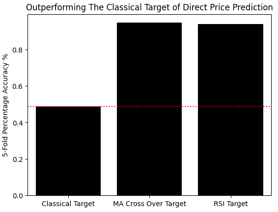
Figure 1: We are making improvements over the classical task of direct price prediction, by modelling the relationship between our strategy and the market

Finally, we can use the scikit-learn random search library to help us build a neural network for our market data. We will begin by initializing our neural network with default settings we wish to keep fixed, such as the shuffle and early stopping parameters.

#Use random search to build a neural network for our market data

#Initialize the model
model = MLPRegressor(shuffle=False,early_stopping=False)


distributions = {'solver':['lbfgs','adam','sgd'],
                 'hidden_layer_sizes':[(X.shape[1],2,10,20),(X.shape[1],30,50,10),(X.shape[1],14,14,14),(X.shape[1],5,20,2),(X.shape[1],1,2,3,4,5,6,10),(X.shape[1],1,14,14,1)],
                 'activation':['relu','identity','logistic','tanh']
                 }

rscv = RandomizedSearchCV(model,distributions,n_jobs=-1,n_iter=50)

rscv.fit(X,data.loc[:,['Target 1','Target 2']])

We are now ready to export our trained neural network to ONNX format. To begin exporting our neural network into our next format, we will first load the ONNX library and then load the necessary converters. Remember that ONNX, which stands for Open Neural Network Exchange, is an open-source protocol that allows us to easily build and export our machine learning models in a manner that is model agnostic.

#Exporting our model to ONNX 
import onnx
from skl2onnx import convert_sklearn
from skl2onnx.common.data_types import FloatTensorType

initial_types = [('float_input',FloatTensorType([1,X.shape[1]]))]
final_types = [('float_output',FloatTensorType([2,1]))]

model = rscv.best_estimator_

model.fit(X,data.loc[:,['Target 1','Target 2']])

onnx_proto = convert_sklearn(model=model,initial_types=initial_types,final_types=final_types,target_opset=12)

onnx.save(onnx_proto,'EURUSD NN MSA.onnx')

To get started viewing our ONNX graph of our neural network, we will first import the Netron library and then simply use the netron.start function and pass the path of the ONNX model in order to view it. 

#Viewing our ONNX graph in netron
import netron
netron.start('../EURUSD NN MSA.onnx')

In Figure 2 below, we have attached the meta-properties of our ONNX model. We can see that our ONNX model has 14 inputs and 2 outputs, both of which are floats, as well as other important metadata such as the producer and the ONNX version.

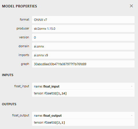
Figure 2: Visualizing the metadata associated with our ONNX model to validate the correct input and output sizes were specified

Our ONNX model represents machine learning models as graphs of computational nodes and edges, which show information being passed from one computational node to the next. In this manner, all machine learning models can be translated into a universal format, which is the ONNX graph, depicted below in Figure 3. This graph represents our neural network that we built using the random search procedure provided by the sklearn library.

Figure 3: Visualizing the computational graph that represents our deep neural network using the Netron library

Building Our Expert Advisor in MQL5

The first step in building our Expert Advisor is to load the ONNX model that we created in the previous step.

//+------------------------------------------------------------------+
//|                                                   MSA Test 1.mq5 |
//|                                               Gamuchirai Ndawana |
//|                    https://www.mql5.com/en/users/gamuchiraindawa |
//+------------------------------------------------------------------+
#property copyright "Gamuchirai Ndawana"
#property link      "https://www.mql5.com/en/users/gamuchiraindawa"
#property version   "1.00"

//+------------------------------------------------------------------+
//| ONNX Model                                                       |
//+------------------------------------------------------------------+
#resource "\\Files\\EURUSD NN MSA.onnx" as uchar onnx_buffer[];

The column means and standard deviations that we measured in Python for each column will be stored in appropriate arrays named Z1 and Z2. Recall that we are going to use these values to scale and standardize each of our inputs before getting predictions from our ONNX model.

//+------------------------------------------------------------------+
//| ONNX Parameters                                                  |
//+------------------------------------------------------------------+
double Z1[] = { 1.18932220e+00,  1.19077958e+00,  1.18786462e+00,  1.18931542e+00,
                1.18994040e+00,  1.18994674e+00,  4.94395259e+01, -4.99204879e-04,
                -5.00701302e-04, -4.97575935e-04, -4.98995739e-04, -4.70848300e-04,
                -4.70289373e-04, -1.84697724e-02
                };

double Z2[] = {1.09599015e-01, 1.09698934e-01, 1.09479324e-01, 1.09593123e-01,
               1.09413744e-01, 1.09419007e-01, 1.00452009e+01, 1.31269558e-02,
               1.31336302e-02, 1.31513465e-02, 1.31174740e-02, 6.88794916e-03,
               6.89036979e-03, 1.28550006e+01
              };

Important system constants will be defined and maintained throughout the lifetime of our program. Remember that these constants were selected in the previous discussion using our genetic optimizer.

//+------------------------------------------------------------------+
//| System constants                                                 |
//+------------------------------------------------------------------+
#define MA_SHIFT         0
#define MA_TYPE          MODE_EMA
#define RSI_PRICE        PRICE_CLOSE
#define ONNX_INPUTS      14
#define ONNX_OUTPUTS     2
#define HORIZON 38 

Important strategy parameters, such as the moving average period and the RSI period, were selected for us using the genetic optimizer, and we will keep them constant throughout our program.

//+------------------------------------------------------------------+
//| Strategy Parameters                                              |
//+------------------------------------------------------------------+
int             MA_PERIOD                       =        100;  //Moving Average Period
int             RSI_PERIOD                      =         24;  //RSI Period
ENUM_TIMEFRAMES STRATEGY_TIME_FRAME             =  PERIOD_H3;  //Strategy Timeframe
int             HOLDING_PERIOD                  =         38;  //Position Maturity Period

We require quite a number of dependencies in order for our application to be complete. Some dependencies, such as the trade library, should be obvious to readers. Others, such as the strategies we developed together in our sister series of articles, should also be familiar to you by now if you have been following along. Otherwise, the strategies we are loading are necessary for our trading application to run.

//+------------------------------------------------------------------+
//| Dependencies                                                     |
//+------------------------------------------------------------------+
#include <Trade\Trade.mqh>
#include <VolatilityDoctor\Time\Time.mqh>
#include <VolatilityDoctor\Trade\TradeInfo.mqh>
#include <VolatilityDoctor\Strategies\OpenCloseMACrossover.mqh>
#include <VolatilityDoctor\Strategies\RSIMidPoint.mqh>

We will have important global variables that are going to be used throughout our program, but fortunately, we only require a handful of them. For example, we require global variables for some of the custom classes that we have built, such as the trade and time classes, the RSI strategy, and the crossover strategy classes. Other global variables will be necessary for us to get readings from our ONNX model and to store the predictions it makes

//+------------------------------------------------------------------+
//| Global Variables                                                 |
//+------------------------------------------------------------------+
//--- Custom Types
CTrade               Trade;
Time                 *TradeTime;
TradeInfo            *TradeInformation;
RSIMidPoint          *RSIMid;
OpenCloseMACrossover *MACross;
long                 onnx_model;
vectorf onnx_output;

//--- Our handlers for our indicators
int ma_handle,ma_o_handle,rsi_handle;

//--- Data structures to store the readings from our indicators
double ma_reading[],ma_o_reading[],rsi_reading[];

//--- System Types
int                  position_timer;

Whenever our application is initialized for the first time, we will create new instances of the dynamic objects that we need. For example, we have a class dedicated to keeping track of time and trading information. We will create new instances of this class, as well as new instances of the appropriate indicator handlers that we will need. From there, we will create our ONNX model from the buffer that we loaded and validate that the model has been loaded correctly.

//+------------------------------------------------------------------+
//| Expert initialization function                                   |
//+------------------------------------------------------------------+
int OnInit()
  {
//--- Create dynamic instances of our custom types
   TradeTime        = new Time(Symbol(),STRATEGY_TIME_FRAME);
   TradeInformation = new TradeInfo(Symbol(),STRATEGY_TIME_FRAME);
   MACross          = new OpenCloseMACrossover(Symbol(),STRATEGY_TIME_FRAME,MA_PERIOD,MA_SHIFT,MA_TYPE);
   RSIMid           = new RSIMidPoint(Symbol(),STRATEGY_TIME_FRAME,RSI_PERIOD,RSI_PRICE);
   onnx_model       = OnnxCreateFromBuffer(onnx_buffer,ONNX_DEFAULT);
   onnx_output      = vectorf::Zeros(ONNX_OUTPUTS);

//---Setup our technical indicators
   ma_handle        = iMA(_Symbol,STRATEGY_TIME_FRAME,MA_PERIOD,0,MA_TYPE,PRICE_CLOSE);
   ma_o_handle      = iMA(_Symbol,STRATEGY_TIME_FRAME,MA_PERIOD,0,MA_TYPE,PRICE_OPEN);
   rsi_handle       = iRSI(_Symbol,STRATEGY_TIME_FRAME,RSI_PERIOD,RSI_PRICE);
   if(onnx_model != INVALID_HANDLE)
     {
      Print("Preparing ONNX model");

      ulong input_shape[] = {1,ONNX_INPUTS};

      if(!OnnxSetInputShape(onnx_model,0,input_shape))
        {
         Print("Failed To Specify ONNX model input shape");
         return(INIT_FAILED);
        }

      ulong output_shape[] = {ONNX_OUTPUTS,1};

      if(!OnnxSetOutputShape(onnx_model,0,output_shape))
        {
         Print("Failed To Specify ONNX model output shape");
         return(INIT_FAILED);
        }
     }

//--- Everything was fine
   Print("Successfully loaded all components for our Expert Advisor");
   return(INIT_SUCCEEDED);
  }
//--- End of OnInit Scope

When our application is no longer in use, we will delete any memory that we are no longer using and free up those resources for other applications, in order to safely deactivate our application.

//+------------------------------------------------------------------+
//| Expert deinitialization function                                 |
//+------------------------------------------------------------------+
void OnDeinit(const int reason)
  {
//--- Delete the dynamic objects
   delete TradeTime;
   delete TradeInformation;
   delete MACross;
   delete RSIMid;
   OnnxRelease(onnx_model);
   IndicatorRelease(ma_handle);
   IndicatorRelease(ma_o_handle);
   IndicatorRelease(rsi_handle);
  }
//--- End of Deinit Scope

Whenever new price levels are received in the OnTick and the OnExpertStart function, we will first check if a new daily candle has fully formed by calling the new_candle function inside the ChangeTime class. If a candle has indeed been formed, then we will update the parameters of our strategy before checking for an opportunity to trade. If opportunities to trade do exist, we will take them. Otherwise, we will wait for our position to reach maturity before closing it.

//+------------------------------------------------------------------+
//| Expert tick function                                             |
//+------------------------------------------------------------------+
void OnTick()
  {
//--- Check if a new daily candle has formed
   if(TradeTime.NewCandle())
     {
      //--- Update strategy
      Update();

      //--- If we have no open positions
      if(PositionsTotal() == 0)
        {
         //--- Reset the position timer
         position_timer = 0;

         //--- Check for a trading signal
         CheckSignal();
        }

      //--- Otherwise
      else
        {
         //--- The position has reached maturity
         if(position_timer == HOLDING_PERIOD)
            Trade.PositionClose(Symbol());
         //--- Otherwise keep holding
         else
            position_timer++;
        }
     }
  }
//--- End of OnTick Scope

Our update method takes in a few important parameters, such as the forecasting horizon that we selected using our genetic optimizer. From there, it updates the strategies we're using and the technical indicator readings stored in our buffers.

//+------------------------------------------------------------------+
//| Update our technical indicators                                  |
//+------------------------------------------------------------------+
void Update(void)
  {
   int fetch = (HORIZON * 2);

//--- Update the strategy
   RSIMid.Update();
   MACross.Update();

//---Set the values as series
   CopyBuffer(ma_handle,0,0,fetch,ma_reading);
   ArraySetAsSeries(ma_reading,true);
   CopyBuffer(ma_o_handle,0,0,fetch,ma_o_reading);
   ArraySetAsSeries(ma_o_reading,true);
   CopyBuffer(rsi_handle,0,0,fetch,rsi_reading);
   ArraySetAsSeries(rsi_reading,true);
  }
//--- End of Update Scope

Getting a prediction from our ONNX model. To get a prediction from the ONNX model, we use the ONNX run function. But before calling it, we must first update the input variables that will be passed to the model, then scale and standardize these values by subtracting the mean and dividing by the standard deviation.

//+------------------------------------------------------------------+
//| Get A Prediction from our ONNX model                             |
//+------------------------------------------------------------------+
void OnnxPredict(void)
  {
   vectorf   input_variables =
     {
      iOpen(_Symbol,STRATEGY_TIME_FRAME,0),
      iHigh(_Symbol,STRATEGY_TIME_FRAME,0),
      iLow(_Symbol,STRATEGY_TIME_FRAME,0),
      iClose(_Symbol,STRATEGY_TIME_FRAME,0),
      ma_reading[0],
      ma_o_reading[0],
      rsi_reading[0],
      iOpen(_Symbol,STRATEGY_TIME_FRAME,0)   - iOpen(_Symbol,STRATEGY_TIME_FRAME,(0 + HORIZON)),
      iHigh(_Symbol,STRATEGY_TIME_FRAME,0)   - iHigh(_Symbol,STRATEGY_TIME_FRAME,(0 + HORIZON)),
      iLow(_Symbol,STRATEGY_TIME_FRAME,0)    - iLow(_Symbol,STRATEGY_TIME_FRAME,(0 + HORIZON)),
      iClose(_Symbol,STRATEGY_TIME_FRAME,0)  - iClose(_Symbol,STRATEGY_TIME_FRAME,(0 + HORIZON)),
      ma_reading[0] - ma_reading[(0 + HORIZON)],
      ma_o_reading[0] - ma_o_reading[(0 + HORIZON)],
      rsi_reading[0] - rsi_reading[(0 + HORIZON)]
     };

   for(int i = 0; i < ONNX_INPUTS;i++)
     {
      input_variables[i] = ((input_variables[i] - Z1[i])/ Z2[i]);
     }

   OnnxRun(onnx_model,ONNX_DEFAULT,input_variables,onnx_output);
  }

Checking for a trading signal using our crossover strategy begins by first getting a prediction from the ONNX model. The model will predict which strategy it believes will be most profitable. From there, we check that particular strategy to see if there is a corresponding entry signal available. We only enter a signal if the model expects the strategy to be profitable and the strategy is offering us a valid trading opportunity.

//+------------------------------------------------------------------+
//| Check for a trading signal using our cross-over strategy         |
//+------------------------------------------------------------------+
void CheckSignal(void)
  {

   OnnxPredict();

//--- MA Strategy is profitable
   if((onnx_output[0] > 0.5) && (onnx_output[1] < 0.5))
     {
      //--- Long positions when the close moving average is above the open
      if(MACross.BuySignal())
        {
         Trade.Buy(TradeInformation.MinVolume(),Symbol(),TradeInformation.GetAsk(),0,0,"");
         return;
        }

      //--- Otherwise short
      else
         if(MACross.SellSignal())
           {
            Trade.Sell(TradeInformation.MinVolume(),Symbol(),TradeInformation.GetBid(),0,0,"");
            return;
           }
     }

//--- RSI strategy is profitable
   else
      if((onnx_output[0] < 0.5) && (onnx_output[1] > 0.5))
        {

         if(RSIMid.BuySignal())
           {
            Trade.Buy(TradeInformation.MinVolume(),Symbol(),TradeInformation.GetAsk(),0,0,"");
            return;
           }

         //--- Otherwise short
         else
            if(MACross.SellSignal())
              {
               Trade.Sell(TradeInformation.MinVolume(),Symbol(),TradeInformation.GetBid(),0,0,"");
               return;
              }
        }
  }
//--- End of CheckSignal Scope

Towards the end of our system, we will undefine all system constants that we defined at the beginning of our application.

//+------------------------------------------------------------------+
//| Undefine system constants                                        |
//+------------------------------------------------------------------+
#undef MA_SHIFT
#undef RSI_PRICE
#undef MA_TYPE
#undef ONNX_INPUTS
#undef ONNX_OUTPUTS
#undef HORIZON
//+------------------------------------------------------------------+

Selecting the appropriate back testing days is straightforward. Recall that we want to test our new application during the forward testing phase used in our previous test. Therefore, the test dates have been adjusted accordingly.

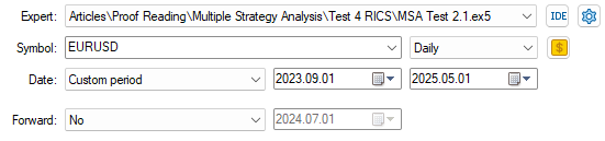
Figure 4: Selecting our back test days so that they align with the forward test we performed earlier

As always, we want to use the most realistic settings possible, so we choose the random delay setting.

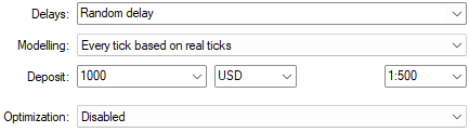
Figure 5: Selecting our modelling conditions to be based on "Random Delay" for the most realistic settings possible

Now, to my surprise, the new settings applied to our application—by including statistical models—actually degraded our performance considerably. This is normally a strong indication that something has gone wrong in our plan.

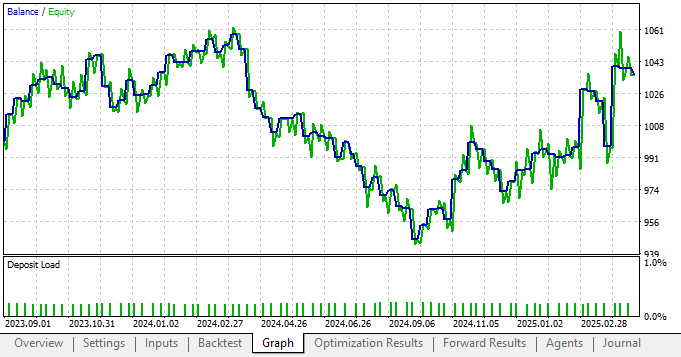
Figure 6: The new equity curve we have produced is in poor health when compared to our performance without statistical modelling

By taking a closer look at the detailed analysis of our application’s performance, we see that the total net profit has fallen along with the Sharpe ratio, which are not good signs. This shows that our application is not receiving the intended benefits of the statistical modeling tools we chose.

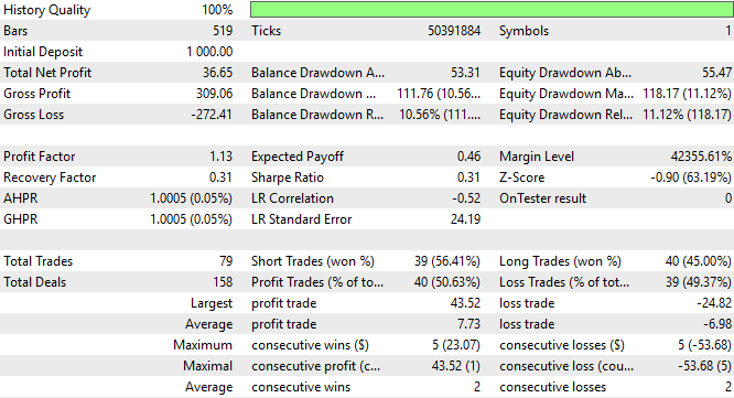
Figure 7: A detailed analysis of the performance of our new trading strategy that relies on statistical models

Revising Our Market Data in Python

Upon further revision of our market data in Python, I wanted to take a closer look at what could be the source of error. So I started by importing the standard libraries we use to visualize market data. I then plotted the cumulative sum of some of the returns generated by the two strategies, and immediately the problem became clear.

import numpy as np
import seaborn as sns
import matplotlib.pyplot as plt

As we can see from the plot below, our two strategies have remarkably similar characteristics and slopes. The two strategies tend to rise and fall in unison, almost as if we were following one strategy.

fig , axs = plt.subplots(2,1,sharex=True)

fig.suptitle('Visualizing The Individual Cumulative Return of our 2 Strategies')

sns.lineplot(data['Return 1'].cumsum(),ax=axs[0],color='black')

sns.lineplot(data['Return 2'].cumsum(),ax=axs[1],color='black')

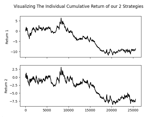
Figure 8: Our Genetic Optimizer appears to have selected highly correlated strategies and assigned them the largest voting weights

Additionally, when we plot the rolling amount of risk in the returns generated by our strategies, we see another cause for concern. The risk profile for our two strategies is almost indistinguishable from that of the market itself. Again, it appears that we are simply using the same strategy. It’s hard to distinguish between strategy one and strategy two if I had not labeled the columns of our plot.

fig , axs = plt.subplots(3,1,sharex=True)

fig.suptitle('Visualizing The Risk In Our 2 Strategies')

sns.lineplot(data['Return'].rolling(window=HORIZON).var(),ax=axs[0],color='black')
axs[0].axhline(data['Return'].var(),color='red',linestyle=':')

sns.lineplot(data['Return 1'].rolling(window=HORIZON).var(),ax=axs[1],color='black')
axs[1].axhline(data['Return 1'].var(),color='red',linestyle=':')

sns.lineplot(data['Return 2'].rolling(window=HORIZON).var(),ax=axs[2],color='black')
axs[2].axhline(data['Return 2'].var(),color='red',linestyle=':')

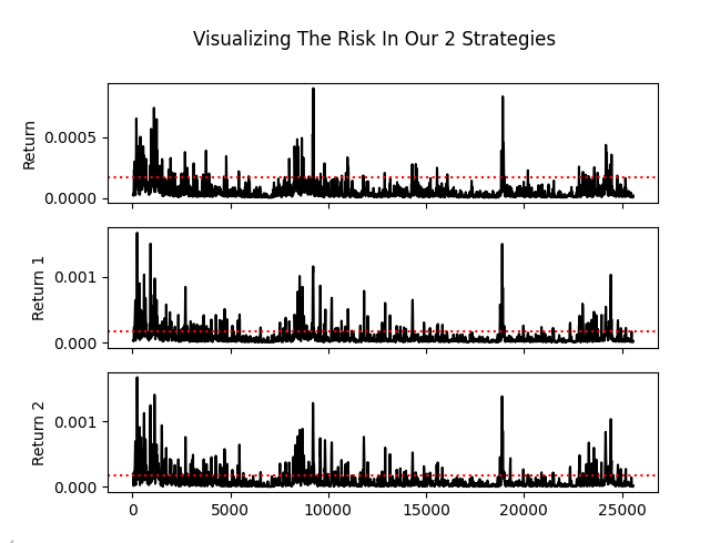
Figure 9: The 2 strategies are almost identical in their levels of risk and reward, this undermines the idea behind multiple strategy analysis

The final nail in the coffin is buried when we calculate the correlation matrix produced by the three returns: the market return, the return from the moving average crossover strategy, and the return from our RSI strategy. We can clearly see that the moving average crossover and RSI strategy have a correlation of about 0.75, which is very strong. This was the final suggestion that convinced me the genetic optimizer was not necessarily adjusting the vote weights to maximize profitability. Rather, it appears that it was tuning the weights to isolate truly correlated strategies—because that makes its job easier.

plt.title('Correlation Between Market Return And Strategy Returns')
sns.heatmap(data.loc[:,['Return','Return 1','Return 2']].corr(),annot=True)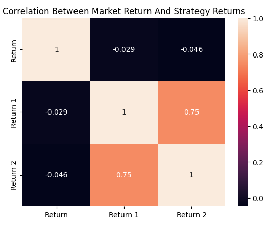

Figure 10: The correlation matrix produced by our trading strategies and the EURUSD market

Making Improvements

Armed with what we know now, we can try again to improve our application. First, we will revert to the earlier version of our trading strategy that included all three strategies we want to use.  

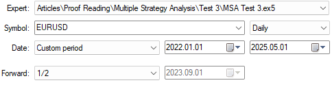
Figure 11: Selecting the back test days for our optimization procedure

As always, we will use random delay settings for our back test.

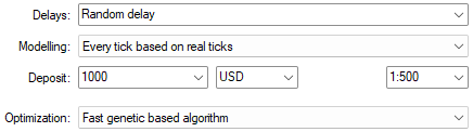
Figure 12: Ensure that you use "Random delay" if you intend to follow along

However, unlike in earlier tests, we will now fix all vote weights to 1 to ensure that the genetic optimizer can only make changes that increase the overall profitability of the strategy. Additionally, we want to force the optimizer to use all three strategies and not cherry-pick correlated ones, as that goes against our intended outcome.

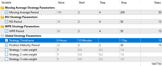
Figure 13: Remember that this time we want to fix all our vote weights at 1, because we suspect the Genetic Optimizer is out smarting us

Upon reviewing the optimization results, we can already see improvements from the initial vectors we performed. Initially, we were observing profitability levels somewhere around $40 to $50 when using all three strategies. However, we are now seeing clear improvements in profitability.

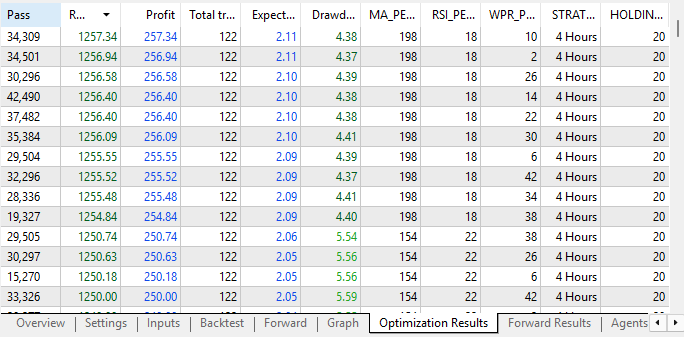
Figure 14: Our optimization results have improved considerably from the previous iteration

Additionally, when we consider the forward test results, we again see increased profit levels. Our tests are now profitable both in the back test and the forward test, which is a strong sign of stability in the configuration. Most importantly, our genetic optimizer is now able to give us batches of strategy configurations that were profitable in both tests. These were the results we were failing to obtain earlier when we allowed the optimizer to alter the weights as it chose. This reinforces our belief that our application is stable in this configuration.

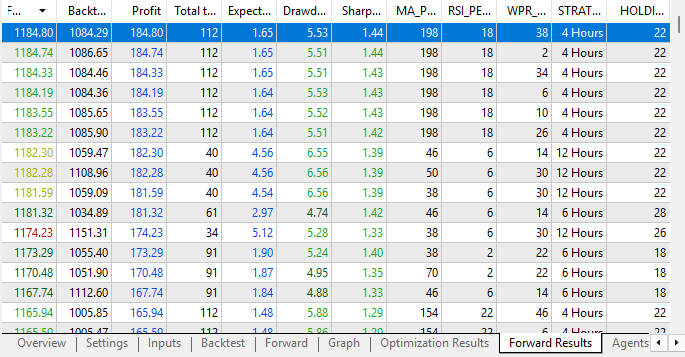
Figure 15: Our Forward results are now demonstrating strong signs of stability and profitability

Lastly, when we run a backtest using the most profitable settings we found from the forward results, we can clearly see that our new parameter settings are profitable in both back test and forward test, with an upward trend—which is what we want to see.

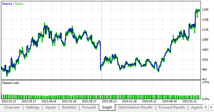
Figure 16: The equity curve produced by our new trading strategy with fixed votes is considerably more profitable

Conclusion

From this discussion, we’ve learned several valuable lessons. First, we’ve seen that the challenge of reward hacking is pervasive and can occur whether we’re aware of it or not. Our AI tools—such as genetic optimizers—are fast and smart, sometimes even smarter than us, and we must always remain vigilant to ensure these tools aren’t outsmarting us by generating invalid solutions that merely satisfy the success conditions we’ve defined.

By carefully reviewing the returns of the strategies selected by the optimizer, we’ve learned that we must avoid selecting correlated strategies, as this defeats the purpose of a multi-strategy analysis.

The reader should note that genetic optimizers are constrained only by the amount of time we are willing to spend. Otherwise, our discussion does not necessarily provide evidence that the MetaTrader 5 genetic optimizer will always hack the rewards given to it. Because we selected only a small number of strategies and performed this optimization just once, there is always the possibility that repeating the process would yield different results.

Rather, this is evidence that I, the writer, may not have been careful enough in how I framed the problem for the genetic optimizer. A better approach would have been to first force the optimizer to use all available strategies, and then adjust the voting weights more thoughtfully.

Most importantly, we conclude this exercise knowing that in our next article, we must carefully consider how to outperform the profitability achieved using uniform weights of 1. The performance we obtained with these uniform weights serves as a solid benchmark—one that we aim to exceed in our upcoming discussion using the statistical models we originally intended to apply in this article.

File Name	File Description
Fetch Data MSA.mq5	The MQL5 script we used to fetch data on the 2 strategies our Genetic Optimizer selected.
MSA Test 2.1.mq5	The Expert Advisor we built using the 2 strategies selected, and our ONNX model in unison.
Analyzing Multiple Strategies I.ipynb	The Jupyter Notebook we wrote together to analyze the market data we fetched using our MQL5 script.
EURUSD NN MSA.onnx	Our deep neural network that we built using the sklearn random-search library.