
Neural Networks in Trading: A Complex Trajectory Prediction Method (Traj-LLM)

Introduction
Forecasting future price movements in financial markets plays a critical role in traders' decision-making processes. High-quality forecasts enable traders to make more informed decisions and minimize risks. However, forecasting future price trajectories faces numerous challenges due to the chaotic and stochastic nature of the markets. Even the most advanced forecasting models often fail to adequately account for all the factors influencing market dynamics, such as sudden shifts in participant behavior or unexpected external events.
In recent years, the development of artificial intelligence, particularly in the field of large language models (LLMs), has opened new avenues for solving a variety of complex tasks. LLMs have demonstrated remarkable capabilities in processing complex information and modeling scenarios in ways that resemble human reasoning. These models are successfully applied in various fields, from natural language processing to time series forecasting, making them promising tools for analyzing and predicting market movements.
I would like to introduce you to the Traj-LLM algorithm, as described in the paper "Traj-LLM: A New Exploration for Empowering Trajectory Prediction with Pre-trained Large Language Models". Traj-LLM was developed to solve tasks in the field of autonomous vehicle trajectory prediction. The authors propose using LLMs to enhance the accuracy and adaptability of forecasting future trajectories of traffic participants.
Moreover, Traj-LLM combines the power of large language models with innovative approaches for modeling temporal dependencies and interactions between objects, enabling more accurate trajectory predictions even under complex and dynamic conditions. This model not only improves forecasting accuracy but also offers new ways to analyze and understand potential future scenarios. We expect that employing the methodology proposed by the authors will be effective in addressing our tasks and will enhance the quality of our forecasts for future price movements.
1. Traj-LLM Algorithm
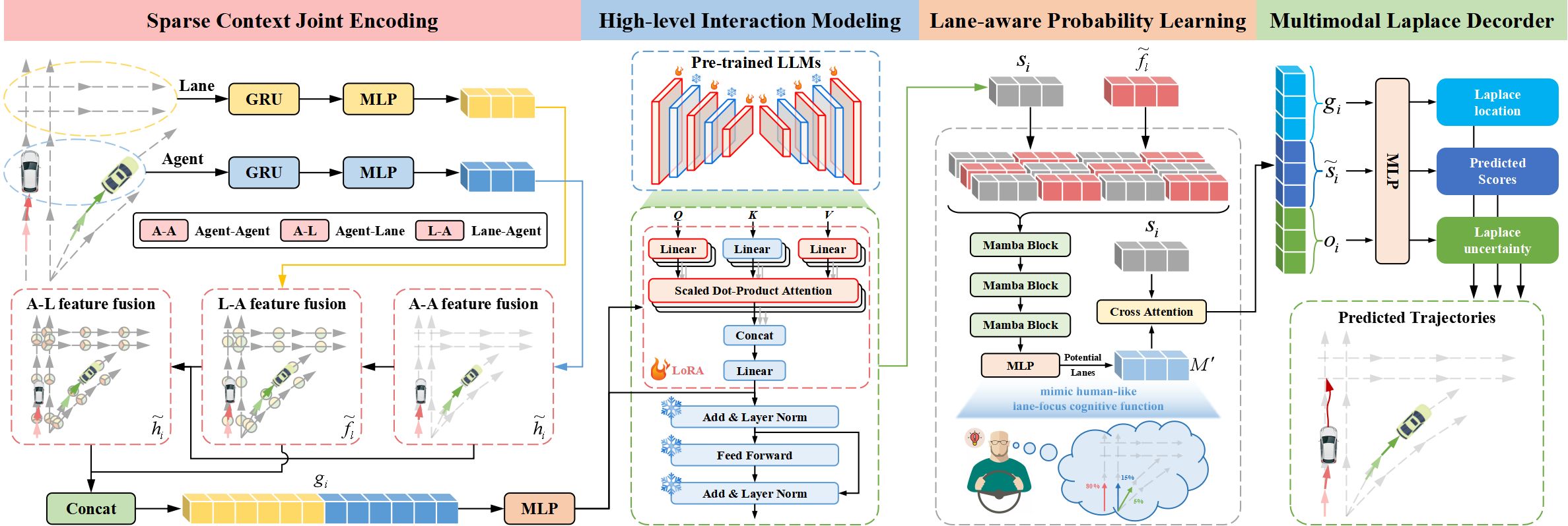
The Traj-LLM architecture consists of four integral components:
- Sparse contextual joint encoding,
- High-level interaction modeling,
- Lane-aware probabilistic learning,
- Laplace multi-modal decoder.
The authors of Traj-LLM method suggest using LLM capabilities for trajectory prediction, eliminating the need for explicit real-time feature engineering. The sparse contextual joint encoding initially transforms agent and scene features into a form interpretable by LLMs. These representations are then input into pre-trained LLMs to handle high-level interaction modeling. To mimic human-like cognitive functions and further enhance scene understanding in Traj-LLM, lane-aware probabilistic learning is introduced via a Mamba module. Finally, the Laplace multi-modal decoder is employed to generate reliable predictions.
The first step in Traj-LLM is encoding the scene's spatio-temporal raw data, such as agent states and lane information. For each of these, an embedding model comprising a recurrent layer and MLP is used to extract multi-dimensional features. The resulting tensors hi and fl are then passed into a Fusion submodule, facilitating complex information exchange between agent states and lanes in localized areas. This process uses a token embedding mechanism to align with the LLM architecture.
Specifically, the fusion process employs a multi-head Self-Attention mechanism to merge Agent-Agent features. Additionally, merging Agent-Lane and Lane-Agent features includes updating Agent and Lane views using a multi-head cross-attention mechanism with skip connections. Formally, this process can be represented as follows:
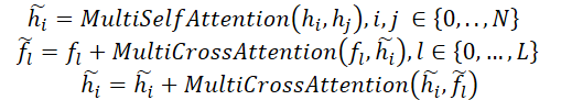
Afterward, hi and fl are combined to form sparse contextual joint encodings gi, intuitively capturing dependencies relevant to the local receptive fields of vectorized entities. This encoding approach is designed to enable LLMs to effectively interpret trajectory data, thus extending LLM capabilities.
Trajectory transitions follow patterns governed by high-level constraints derived from various scene elements. To study these interactions, the authors explore LLMs' abilities to model dependencies inherent in trajectory prediction tasks. Despite similarities between trajectory data and natural language texts, directly using LLMs to process sparse contextual joint encodings is deemed inefficient. Because pre-trained LLMs are primarily optimized for text data. One alternative proposal is a comprehensive retraining of all LLMs. This process requires significant computational resources, making it somewhat unfeasible. Another more effective solution is to use the Parameter-Efficient Fine-Tuning method (PEFT) to fine-tune pre-trained LLMs.
Traj-LLM authors use parameters from pretrained NLP transformer architectures, particularly GPT-2, for high-level interaction modeling. They propose to freeze all pre-trained parameters and introduce new trainable ones using a Low-Rank Adaptation technique (LoRA). LoRA is applied to Query and Key entities of the LLM attention mechanism.
Thus, the sparse contextual joint encodings gi are input into an LLM consisting of a series of pre-trained Transformer blocks enhanced with LoRA. This procedure yields high-level interaction representations zi.
![]()
The outputs of the pre-trained LLM are transformed via an MLP to match the dimensions of gi, resulting in final high-level interaction states si.
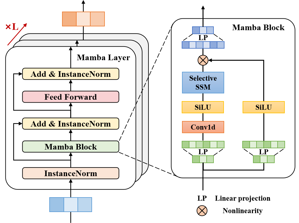
Most experienced drivers focus on a limited number of relevant lane segments that significantly influence their future actions. To replicate this human-like cognitive function and further improve scene understanding in Traj-LLM, the method authors use lane-aware probabilistic learning to continuously assess the likelihood of aligning motion states with lane segments. The model aligns the target agent's trajectory with lane information at each time step t∈{1,…,tf} using a Mamba layer. Acting as a selective structured state-space model (SSM), Mamba refines and generalizes relevant information. This is similar to how human drivers selectively process crucial environmental cues such as potential lanes to make their choices.
In the proposed architecture, the Mamba layer includes a Mamba block, triple-layer normalization, and a position-wise feed-forward network. The Mamba block first expands the dimensionality via linear projections, creating distinct representations for two parallel data flows. One branch undergoes convolution and SiLU activation to capture lane-aware dependencies. At its core, the Mamba block incorporates a selective state-space model with discretized parameters, based on the input data. To improve stability, instance normalization and residual connections are added, resulting in latent representations.
Subsequently, a position-wise FeedForward network enhances modeling of lane-aligned assessments in the hidden dimension. Again, instance normalization and residual connections are applied to produce lane-aware training vectors, which are then passed to an MLP layer.
As mentioned, experienced drivers focus on key lane segments to make efficient decisions. Therefore, top candidate lanes are carefully selected and combined into a set ℳ.
Lane-aware probabilistic learning is modeled as a classification task, using binary cross-entropy loss ℒlane to optimize probability estimation.
Authors' visualization of the Traj-LLM method is presented below.
2. Implementation in MQL5
After considering the theoretical aspects of the Traj-LLM method, we move on to the practical part of our article, in which we implement our vision of the proposed approaches using MQL5. The Traj-LLM algorithm is a complex framework that integrates multiple architectural components, some of which we have already encountered in previous work. Thus, we can utilize existing modules when constructing the algorithm. However, additional modifications will be necessary.
2.1 Adjusting the LSTM Block Algorithm
Let's look at the visualization of the Traj-LLM method presented above. Raw input data first passes through the sparse contextual joint encoding block, comprising a recurrent layer and MLP. Our library already includes the recurrent layer CNeuronLSTMOCL. However, it processes the input data as a single, unified environmental state representation. In contrast, the method authors propose independent encoding of individual agents and lane states. Therefore, we must organize independent encoding for each data channel. Well, we could instantiate a separate CNeuronLSTMOCL object for each channel. However, this would lead to an uncontrollable increase in internal objects and sequential processing, negatively affecting model performance.
A second solution is to modify the existing CNeuronLSTMOCL recurrent layer class. This requires changes on the OpenCL program side. The feed-forward pass of our recurrent layer is implemented in the LSTM_FeedForward kernel. To implement operations within univariate sequences, we we will not make changes to the external parameters of the kernel. To organize parallel processing of data of individual univariate sequences, we will add one more dimension to the task space.
__kernel void LSTM_FeedForward(__global const float *inputs, int inputs_size,
                               __global const float *weights,
                               __global float *concatenated,
                               __global float *memory, __global float *output)
  {
   uint id = (uint)get_global_id(0);
   uint total = (uint)get_global_size(0);
   uint id2 = (uint)get_local_id(1);
   uint idv = (uint)get_global_id(2);
   uint total_v = (uint)get_global_size(2);
Let me remind you that the operation of the LSTM block is based on four entities, whose values are computed by internal layers:
- Forget Gate — responsible for discarding irrelevant information
- Input Gate — responsible for incorporating new information
- Output Gate — responsible for generating the output signal
- New Content — representing the candidate values for updating the cell state
The algorithm for computing these entities is uniform and follows the structure of a fully connected layer. The only difference lies in the activation functions applied at each stage. Therefore, in our implementation, we have designed the computation of these entities to be processed in parallel threads within a workgroup. To enable data exchange between threads, we use an array allocated in local memory.
__local float Temp[4];
Next we define the shift constants in the global data buffers.
   float sum = 0;
   uint shift_in = idv * inputs_size;
   uint shift_out = idv * total;
   uint shift = (inputs_size + total + 1) * (id2 + id);
Please pay attention to the following points. We implement the process of working of the recurrent block with independent channels. However, according to the Traj-LLM algorithm construction logic, all independent information channels contain comparable data, whether it is information on the state of various agents or existing traffic lanes. Therefore, it is quite logical to use one weight matrix to encode information from different data channels, which will allow us to obtain comparable embeddings at the output.
Thus, the channel identifier affects the offset in the source and result buffers. But it does not affect the shift in the weight matrix.
Next, we create a loop to calculate the weighted sum of the hidden state.
   for(uint i = 0; i < total; i += 4)
     {
      if(total - i > 4)
         sum +=
            dot((float4)(output[shift_out + i], output[shift_out + i + 1],
                         output[shift_out + i + 2], output[shift_out + i + 3]),
                (float4)(weights[shift + i], weights[shift + i + 1],
                         weights[shift + i + 2], weights[shift + i + 3]));
      else
         for(uint k = i; k < total; k++)
            sum += output[shift_out + k] * weights[shift + k];
     }
And we add the influence of the input data.
   shift += total;
   for(uint i = 0; i < inputs_size; i += 4)
     {
      if(total - i > 4)
         sum +=
            dot((float4)(inputs[shift_in + i], inputs[shift_in + i + 1],
                         inputs[shift_in + i + 2], inputs[shift_in + i + 3]),
                (float4)(weights[shift + i], weights[shift + i + 1],
                         weights[shift + i + 2], weights[shift + i + 3]));
      else
         for(uint k = i; k < total; k++)
            sum += inputs[shift_in + k] * weights[shift + k];
     }
   sum += weights[shift + inputs_size];
We apply the corresponding activation function to the obtained value.
   if(isnan(sum) || isinf(sum))
      sum = 0;
   if(id2 < 3)
      sum = Activation(sum, 1);
   else
      sum = Activation(sum, 0);
After that, we save the results of the operations and synchronize the workgroup threads.
   Temp[id2] = sum;
   concatenated[4 * shift_out + id2 * total + id] = sum;
//---
   barrier(CLK_LOCAL_MEM_FENCE);
Now we just need to calculate the result of the LSTM block work that is simultaneously the hidden state of a given cell.
   if(id2 == 0)
     {
      float mem = memory[shift_out + id + total_v * total] = memory[shift_out + id];
      float fg = Temp[0];
      float ig = Temp[1];
      float og = Temp[2];
      float nc = Temp[3];
      //---
      memory[shift_out + id] = mem = mem * fg + ig * nc;
      output[shift_out + id] = og * Activation(mem, 0);
     }
  }
The results of the operations are saved in the corresponding elements of the global data buffers.
We made similar edits to the backpropagation pass kernels. The most significant of them were in the LSTM_HiddenGradient kernel. As in the feed-forward kernel, we do not change the composition of external parameters and only adjust the task space.
__kernel void LSTM_HiddenGradient(__global float *concatenated_gradient, __global float *inputs_gradient,
                                  __global float *weights_gradient, __global float *hidden_state,
                                  __global float *inputs, __global float *weights, __global float *output,
                                  const int hidden_size, const int inputs_size)
  {
   uint id = get_global_id(0);
   uint total = get_global_size(0);
   uint idv = (uint)get_global_id(1);
   uint total_v = (uint)get_global_size(1);
All independent channels work with one weight matrix. Therefore, for the weighting coefficients we have to collect the error gradients from all independent channels. Each data channel operates in its own thread, which we will combine into working groups. To exchange data between threads, we will use an array in local memory.
   __local float Temp[LOCAL_ARRAY_SIZE];
   uint ls = min(total_v, (uint)LOCAL_ARRAY_SIZE);
Next we define offsets in the data buffers.
   uint shift_in = idv * inputs_size;
   uint shift_out = idv * total;
   uint weights_step = hidden_size + inputs_size + 1;
We create a loop over the concatenated buffer of the input data. First we just update the hidden state.
   for(int i = id; i < (hidden_size + inputs_size); i += total)
     {
      float inp = 0;
      if(i < hidden_size)
        {
         inp = hidden_state[shift_out + i];
         hidden_state[shift_out + i] = output[shift_out + i];
        }
And then we determine the error gradient at the input level.
      else
        {
         inp = inputs[shift_in + i - hidden_size];
         float grad = 0;
         for(uint g = 0; g < 3 * hidden_size; g++)
           {
            float temp = concatenated_gradient[4 * shift_out + g];
            grad += temp * (1 - temp) * weights[i + g * weights_step];
           }
         for(uint g = 3 * hidden_size; g < 4 * hidden_size; g++)
           {
            float temp = concatenated_gradient[4 * shift_out + g];
            grad += temp * (1 - pow(temp, 2.0f)) * weights[i + g * weights_step];
           }
         inputs_gradient[shift_in + i - hidden_size] = grad;
        }
Here we also calculate the error gradient at the weight level. First, we reset the values of the local array.
      for(uint g = 0; g < 3 * hidden_size; g++)
        {
         float temp = concatenated_gradient[4 * shift_out + g];
         if(idv < ls)
            Temp[idv % ls] = 0;
         barrier(CLK_LOCAL_MEM_FENCE);
Make sure to synchronize the work of the workgroup threads.
Next, we collect the total error gradient from all data channels. In the first step, we save individual values in a local array.
         for(uint v = 0; v < total_v; v += ls)
           {
            if(idv >= v && idv < v + ls)
               Temp[idv % ls] += temp * (1 - temp) * inp;
            barrier(CLK_LOCAL_MEM_FENCE);
           }
We assume that there will be a relatively small number of independent channels in the analyzed data. Therefore, we collect the sum of the array values in one thread and then save the resulting value in the global data buffer.
         if(idv == 0)
           {
            temp = Temp[0];
            for(int v = 1; v < ls; v++)
               temp += Temp[v];
            weights_gradient[i + g * weights_step] = temp;
           }
         barrier(CLK_LOCAL_MEM_FENCE);
        }
Similarly, we collect the error gradient for the New Content weights.
      for(uint g = 3 * hidden_size; g < 4 * hidden_size; g++)
        {
         float temp = concatenated_gradient[4 * shift_out + g];
         if(idv < ls)
            Temp[idv % ls] = 0;
         barrier(CLK_LOCAL_MEM_FENCE);
         for(uint v = 0; v < total_v; v += ls)
           {
            if(idv >= v && idv < v + ls)
               Temp[idv % ls] += temp * (1 - pow(temp, 2.0f)) * inp;
            barrier(CLK_LOCAL_MEM_FENCE);
           }
         if(idv == 0)
           {
            temp = Temp[0];
            for(int v = 1; v < ls; v++)
               temp += Temp[v];
            weights_gradient[i + g * weights_step] = temp;
           }
         barrier(CLK_LOCAL_MEM_FENCE);
        }
     }
Please note here that during the execution of the main loop operations, we lost sight of the Bayesian bias weighting factors. To compute the corresponding error gradients, we implement additional operations according to the above scheme.
   for(int i = id; i < 4 * hidden_size; i += total)
     {
      if(idv < ls)
         Temp[idv % ls] = 0;
      barrier(CLK_LOCAL_MEM_FENCE);
      float temp = concatenated_gradient[4 * shift_out + (i + 1) * hidden_size];
      if(i < 3 * hidden_size)
        {
         for(uint v = 0; v < total_v; v += ls)
           {
            if(idv >= v && idv < v + ls)
               Temp[idv % ls] += temp * (1 - temp);
            barrier(CLK_LOCAL_MEM_FENCE);
           }
        }
      else
        {
         for(uint v = 0; v < total_v; v += ls)
           {
            if(idv >= v && idv < v + ls)
               Temp[idv % ls] += 1 - pow(temp, 2.0f);
            barrier(CLK_LOCAL_MEM_FENCE);
           }
        }
      if(idv == 0)
        {
         temp = Temp[0];
         for(int v = 1; v < ls; v++)
            temp += Temp[v];
         weights_gradient[(i + 1) * weights_step] = temp;
        }
      barrier(CLK_LOCAL_MEM_FENCE);
     }
  }
Special attention should be given to thread synchronization points. Their number must be minimally sufficient to ensure the correct functioning of the algorithm. Excessive synchronization points will degrade the performance and slow down operations. Moreover, improperly placed synchronization points, where not all threads reach them, may cause the program to stop responding.
With this, we conclude our review of the OpenCL code adjustments necessary to organize LSTM block operations under independent data channels. As for specific edits on the side of the main program, I encourage you to explore those independently. The full code of the updated CNeuronLSTMOCL class and all its methods is provided in the attachment.
2.2 Building the Mamba Block
The next step in our preparatory work is the construction of the Mamba block. The name of this block is intentionally reminiscent of the method we discussed in the previous article. The authors of Traj-LLM extend the use of state-space models (SSM) and propose a block architecture that can be compared to a Transformer Encoder. But in this case, Self-Attention is replaced by the Mamba architecture.
To implement the proposed algorithm, we will create a new class CNeuronMambaBlockOCL, whose structure is presented below.
class CNeuronMambaBlockOCL :  public   CNeuronBaseOCL
  {
protected:
   uint              iWindow;
   CNeuronMambaOCL   cMamba;
   CNeuronBaseOCL    cMambaResidual;
   CNeuronConvOCL    cFF[2];
   //---
   virtual bool      feedForward(CNeuronBaseOCL *NeuronOCL) override;
   //---
   virtual bool      calcInputGradients(CNeuronBaseOCL *NeuronOCL) override;
   virtual bool      updateInputWeights(CNeuronBaseOCL *NeuronOCL) override;
   //---

public:
                     CNeuronMambaBlockOCL(void) {};
                    ~CNeuronMambaBlockOCL(void) {};
   //---
   virtual bool      Init(uint numOutputs, uint myIndex, COpenCLMy *open_cl,
                          uint window, uint window_key, uint units_count,
                          ENUM_OPTIMIZATION optimization_type, uint batch);
   //---
   virtual int       Type(void) override  const   {  return defNeuronMambaBlockOCL; }
   //---
   virtual bool      Save(int const file_handle) override;
   virtual bool      Load(int const file_handle) override;
   //---
   virtual bool      WeightsUpdate(CNeuronBaseOCL *source, float tau) override;
   virtual void      SetOpenCL(COpenCLMy *obj) override;
  };
The core functionality will be inherited from the base fully connected layer class CNeuronBaseOCL. We will override the familiar list of virtual methods.
Within the structure of our new class, we can highlight internal objects, whose functionality we will explore step by step as we proceed with method implementation. All objects are declared statically. This allows us to leave the class constructor and destructor "empty". Initialization of all internal objects and variables will be handled inside the Init method.
As mentioned earlier, the Mamba block, by its architecture, resembles a Transformer Encoder. This resemblance is also evident in the parameters of the initialization method, which provide a clear and structured definition of the block's internal architecture.
bool CNeuronMambaBlockOCL::Init(uint numOutputs, uint myIndex, COpenCLMy *open_cl,
                                uint window, uint window_key, uint units_count,
                                ENUM_OPTIMIZATION optimization_type, uint batch)
  {
   if(!CNeuronBaseOCL::Init(numOutputs, myIndex, open_cl, window * units_count, optimization_type, batch))
      return false;
Within the body of the method, we call the method of the same name from the parent class, which already contains a minimally necessary block for parameter validation and the initialization of all inherited objects.
Upon successful execution of the parent class initialization method, we save the data analysis window size in a local variable for further use.
iWindow = window;
Then we move on to initializing internal objects. First we initialize the Mamba state space layer.
   if(!cMamba.Init(0, 0, OpenCL, window, window_key, units_count, optimization, iBatch))
      return false;
This is followed by a fully connected layer, whose buffer we intend to use for storing the normalized results of the selective state-space analysis with residual connection.
   if(!cMambaResidual.Init(0, 1, OpenCL, window * units_count, optimization, iBatch))
      return false;
   cMambaResidual.SetActivationFunction(None);
After that we add a FeedForward block.
   if(!cFF[0].Init(0, 2, OpenCL, window, window, 4 * window, units_count, 1, optimization, iBatch))
      return false;
   cFF[0].SetActivationFunction(LReLU);
   if(!cFF[1].Init(0, 2, OpenCL, 4 * window, 4 * window, window, units_count, 1, optimization, iBatch))
      return false;
   cFF[1].SetActivationFunction(None);
Then we organize the substitution of pointers to data buffers in order to eliminate unnecessary copying operations.
   SetActivationFunction(None);
   SetGradient(cFF[1].getGradient(), true);
//---
   return true;
  }
Note that here we are only replacing the pointer to the error gradient buffer. This is due to the fact that during the feed-forward pass, before transferring the results to the layer output, an additional residual connection and normalization of the obtained results will be organized.
Don't forget to monitor the results of the operations at each step. At the end of the method we return the logical result of the performed operations to the calling program.
After initializing the class object, we move on to constructing the feed-forward pass algorithm, which is implemented in the feedForward method. It is quite straightforward.
bool CNeuronMambaBlockOCL::feedForward(CNeuronBaseOCL *NeuronOCL)
  {
   if(!cMamba.FeedForward(NeuronOCL))
      return false;
In the method parameters, we receive a pointer to the object of the previous layer, which passes us the input data. And in the body of the method, we immediately pass the received pointer to the selective model of the state space.
After successfully completing the operations of the direct pass method of the inner layer, we sum up the obtained results and the original data, followed by normalization of the values.
   if(!SumAndNormilize(cMamba.getOutput(), NeuronOCL.getOutput(), cMambaResidual.getOutput(), iWindow, true))
      return false;
Next comes the FeedForward block.
   if(!cFF[0].FeedForward(cMambaResidual.AsObject()))
      return false;
   if(!cFF[1].FeedForward(cFF[0].AsObject()))
      return false;
We organize the residual connection with subsequent data normalization.
   if(!SumAndNormilize(cMambaResidual.getOutput(), cFF[1].getOutput(), getOutput(), iWindow, true))
      return false;
//---
   return true;
  }
Backpropagation methods also have quite a simple algorithm, and I suggest leaving them for independent study. Let me remind you that in the attachment, you will find the full code of this class and all its methods.
With this we complete the preparatory work and move on to constructing the general algorithm of the Traj-LLM method.
2.3 Assembling Individual Blocks into a Coherent Algorithm
Above we have done the preparatory work and supplemented our library with the missing "building blocks" that we will use to build the Traj-LLM algorithm within the CNeuronTrajLLMOCL class. The structure of the new class is shown below.
class CNeuronTrajLLMOCL :  public CNeuronBaseOCL
  {
protected:
   //--- State Encoder
   CNeuronLSTMOCL                cStateRNN;
   CNeuronConvOCL                cStateMLP[2];
   //--- Variables Encoder
   CNeuronTransposeOCL           cTranspose;
   CNeuronLSTMOCL                cVariablesRNN;
   CNeuronConvOCL                cVariablesMLP[2];
   //--- Context Encoder
   CNeuronLearnabledPE           cStatePE;
   CNeuronLearnabledPE           cVariablesPE;
   CNeuronMLMHAttentionMLKV      cStateToState;
   CNeuronMLCrossAttentionMLKV   cVariableToState;
   CNeuronMLCrossAttentionMLKV   cStateToVariable;
   CNeuronBaseOCL                cContext;
   CNeuronConvOCL                cContextMLP[2];
   //---
   CNeuronMLMHAttentionMLKV      cHighLevelInteraction;
   CNeuronMambaBlockOCL          caMamba[3];
   CNeuronMLCrossAttentionMLKV   cLaneAware;
   CNeuronConvOCL                caForecastMLP[2];
   CNeuronTransposeOCL           cTransposeOut;
   //---
   virtual bool      feedForward(CNeuronBaseOCL *NeuronOCL) override;
   //---
   virtual bool      calcInputGradients(CNeuronBaseOCL *NeuronOCL) override;
   virtual bool      updateInputWeights(CNeuronBaseOCL *NeuronOCL) override;
   //---

public:
                     CNeuronTrajLLMOCL(void) {};
                    ~CNeuronTrajLLMOCL(void) {};
   //---
   virtual bool      Init(uint numOutputs, uint myIndex, COpenCLMy *open_cl,
                          uint window, uint window_key, uint heads, uint units_count, uint forecast,
                          ENUM_OPTIMIZATION optimization_type, uint batch);
   //---
   virtual int       Type(void)   const   {  return defNeuronTrajLLMOCL; }
   //---
   virtual bool      Save(int const file_handle);
   virtual bool      Load(int const file_handle);
   //---
   virtual bool      WeightsUpdate(CNeuronBaseOCL *source, float tau);
   virtual void      SetOpenCL(COpenCLMy *obj);
  };
As can be seen, in the class structure we override the same virtual methods. However, this class is distinguished by a significantly larger number of internal objects, which is quite expected for such a complex architecture. The purpose of these declared objects will become clear as we proceed with the implementation of the class methods.
All internal objects of the class are declared as static. Consequently, the constructor and destructor remain empty. The initialization of all declared objects is performed in the Init method.
In the method parameters we receive the main constants that will be used to initialize the nested objects. Here we see the names of the parameters that are already familiar to us. However, please note that some of them may carry different functionality for individual internal objects.
bool CNeuronTrajLLMOCL::Init(uint numOutputs, uint myIndex, COpenCLMy *open_cl,
                             uint window, uint window_key, uint heads, uint units_count, uint forecast,
                             ENUM_OPTIMIZATION optimization_type, uint batch)
  {
   if(!CNeuronBaseOCL::Init(numOutputs, myIndex, open_cl, window * forecast, optimization_type, batch))
      return false;
Following an already established tradition, the first step within the Init method is to call the parent class method of the same name. As you know, this method already performs basic parameter validation and initialization of all inherited objects. After the successful execution of the parent class method, we proceed to initialize the declared internal objects.
Based on the experience gained from building previous models, we assume that the input to the model is a matrix describing the current market situation. Each row of this matrix contains a set of parameters characterizing an individual market candlestick, including the corresponding values of the analyzed indicators.
According to the Traj-LLM algorithm, the obtained input data are first passed to the Sparse Context Encoder block, which includes an agent encoder and a lane encoder. In our case, these correspond to encoders for environmental states (individual bar data) and historical trajectories of analyzed parameters (indicators).
The state encoder will be constructed from a recurrent block for analyzing individual bars and two subsequent convolutional layers, which will implement the MLP operation within independent information channels.
//--- State Encoder
   if(!cStateRNN.Init(0, 0, OpenCL, window_key, units_count, optimization, iBatch) ||
      !cStateRNN.SetInputs(window))
      return false;
   if(!cStateMLP[0].Init(0, 1, OpenCL, window_key, window_key, 4 * window_key, units_count,
                                                                          optimization, iBatch))
      return false;
   cStateMLP[0].SetActivationFunction(LReLU);
   if(!cStateMLP[1].Init(0, 2, OpenCL, 4 * window_key, 4 * window_key, window_key, units_count,
                                                                          optimization, iBatch))
      return false;
The method parameters include the main constants used for initializing embedded objects. Here, we see familiar parameter names, but it is important to note that some of them may serve different functions for specific internal objects.
//--- Variables Encoder
   if(!cTranspose.Init(0, 3, OpenCL, units_count, window, optimization, iBatch))
      return false;
   if(!cVariablesRNN.Init(0, 4, OpenCL, window_key, window, optimization, iBatch) ||
      !cVariablesRNN.SetInputs(units_count))
      return false;
   if(!cVariablesMLP[0].Init(0, 5, OpenCL, window_key, window_key, 4 * window_key, window,
                                                                         optimization, iBatch))
      return false;
   cVariablesMLP[0].SetActivationFunction(LReLU);
   if(!cVariablesMLP[1].Init(0, 6, OpenCL, 4 * window_key, 4 * window_key, window_key, window,
                                                                         optimization, iBatch))
      return false;
It is important to note that, according to the Traj-LLM algorithm, a joint analysis of Agents and Lanes is subsequently performed. Therefore, the output of the encoders produces vectors representing individual elements of the sequences (environmental states or historical trajectories of analyzed indicators) of identical dimensions. At the same time, differences in sequence lengths are allowed, since the number of analyzed environmental states is often not equal to the number of analyzed parameters describing those states.
Following the next step in the Traj-LLM algorithm, the outputs of the encoders are passed to the Fusion block, where a comprehensive analysis of the interdependencies between individual sequence elements is carried out using Self-Attention and Cross-Attention mechanisms. However, it is well known that to improve the efficiency of attention mechanisms, positional encoding tags must be added to the sequence elements. To achieve this functionality, we will introduce two trainable positional encoding layers.
//--- Position Encoder
   if(!cStatePE.Init(0, 7, OpenCL, cStateMLP[1].Neurons(), optimization, iBatch))
      return false;
   if(!cVariablesPE.Init(0, 8, OpenCL, cVariablesMLP[1].Neurons(), optimization, iBatch))
      return false;
And only then we analyze the dependencies between individual states in the Self-Attention block.
//--- Context
   if(!cStateToState.Init(0, 9, OpenCL, window_key, window_key, heads, heads / 2, units_count, 2, 1,
                                                                                optimization, iBatch))
      return false;
Then we perform cross-dependency analysis in the next 2 cross-attention blocks.
   if(!cStateToVariable.Init(0, 10, OpenCL, window_key, window_key, heads, window_key, heads / 2,
                                                      units_count, window, 2, 1, optimization, iBatch))
      return false;
   if(!cVariableToState.Init(0, 11, OpenCL, window_key, window_key, heads, window_key, heads / 2,
                                                       window, units_count, 2, 1, optimization, iBatch))
      return false;
The enriched representations of states and trajectories are concatenated into a single tensor.
   if(!cContext.Init(0, 12, OpenCL, window_key * (units_count + window), optimization, iBatch))
      return false;
After that the data goes through another MLP.
   if(!cContextMLP[0].Init(0, 13, OpenCL, window_key, window_key, 4 * window_key, window + units_count,
                                                                                   optimization, iBatch))
      return false;
   cContextMLP[0].SetActivationFunction(LReLU);
   if(!cContextMLP[1].Init(0, 14, OpenCL, 4 * window_key, 4 * window_key, window_key, window + units_count,
                                                                                    optimization, iBatch))
      return false;
Next comes the high-level interaction modeling block. Here are the authors of the Traj-LLM method use a pre-trained language model, which we will replace with a Transformer block.
   if(!cHighLevelInteraction.Init(0, 15, OpenCL, window_key, window_key, heads, heads / 2,
                                                        window + units_count, 4, 2, optimization, iBatch))
      return false;
Next comes the cognitive block of learning the probabilities of subsequent movement, taking into account the existing traffic lanes. Here we use 3 consecutive Mamba blocks having the same architectures.
   for(int i = 0; i < int(caMamba.Size()); i++)
     {
      if(!caMamba[i].Init(0, 16 + i, OpenCL, window_key, 2 * window_key, window + units_count,
                                                                         optimization, iBatch))
         return false;
     }
The obtained values are compared with historical trajectories in the cross-attention block.
   if(!cLaneAware.Init(0, 19, OpenCL, window_key, window_key, heads, window_key, heads / 2, window,
                                                  window + units_count, 2, 1, optimization, iBatch))
      return false;
And finally we use MLP to predict subsequent trajectories of independent data channels.
   if(!caForecastMLP[0].Init(0, 20, OpenCL, window_key, window_key, 4 * forecast, window, optimization, iBatch))
      return false;
   caForecastMLP[0].SetActivationFunction(LReLU);
   if(!caForecastMLP[1].Init(0, 21, OpenCL, 4 * forecast, 4 * forecast, forecast, window, optimization, iBatch))
      return false;
   caForecastMLP[1].SetActivationFunction(TANH);
   if(!cTransposeOut.Init(0, 22, OpenCL, window, forecast, optimization, iBatch))
      return false;
Note that the predicted trajectory tensor is transposed to bring the information into the representation of the original data.
   SetOutput(cTransposeOut.getOutput(), true);
   SetGradient(cTransposeOut.getGradient(), true);
   SetActivationFunction((ENUM_ACTIVATION)caForecastMLP[1].Activation());
//---
   return true;
  }
We also use data buffer pointer substitution to avoid unnecessary copy operations. After that we return the logical result of the method operations to the calling program.
After completing the work on the class initialization method, we move on to constructing the feed-forward pass algorithm, which we implement in the feedForward method.
bool CNeuronTrajLLMOCL::feedForward(CNeuronBaseOCL *NeuronOCL)
  {
//--- State Encoder
   if(!cStateRNN.FeedForward(NeuronOCL))
      return false;
   if(!cStateMLP[0].FeedForward(cStateRNN.AsObject()))
      return false;
   if(!cStateMLP[1].FeedForward(cStateMLP[0].AsObject()))
      return false;
In the method parameters we receive a pointer to an object with the initial data, which we immediately pass through the state encoder block.
Then we transpose the original data and encode the historical trajectories of the analyzed parameters describing the state of the environment.
//--- Variables Encoder
   if(!cTranspose.FeedForward(NeuronOCL))
      return false;
   if(!cVariablesRNN.FeedForward(cTranspose.AsObject()))
      return false;
   if(!cVariablesMLP[0].FeedForward(cVariablesRNN.AsObject()))
      return false;
   if(!cVariablesMLP[1].FeedForward(cVariablesMLP[0].AsObject()))
      return false;
We add positional encoding to the obtained data.
//--- Position Encoder
   if(!cStatePE.FeedForward(cStateMLP[1].AsObject()))
      return false;
   if(!cVariablesPE.FeedForward(cVariablesMLP[1].AsObject()))
      return false;
After which we enrich the data with the context of interdependencies.
//--- Context
   if(!cStateToState.FeedForward(cStatePE.AsObject()))
      return false;
   if(!cStateToVariable.FeedForward(cStateToState.AsObject(), cVariablesPE.getOutput()))
      return false;
   if(!cVariableToState.FeedForward(cVariablesPE.AsObject(), cStateToVariable.getOutput()))
      return false;
The enriched data is concatenated into a single tensor.
   if(!Concat(cStateToVariable.getOutput(), cVariableToState.getOutput(), cContext.getOutput(),
                                      cStateToVariable.Neurons(), cVariableToState.Neurons(), 1))
      return false;
And then it is processed by an MLP.
   if(!cContextMLP[0].FeedForward(cContext.AsObject()))
      return false;
   if(!cContextMLP[1].FeedForward(cContextMLP[0].AsObject()))
      return false;
Next comes the block of high-level dependency analysis.
//--- Lane aware
   if(!cHighLevelInteraction.FeedForward(cContextMLP[1].AsObject()))
      return false;
And the state space model.
   if(!caMamba[0].FeedForward(cHighLevelInteraction.AsObject()))
      return false;
   for(int i = 1; i < int(caMamba.Size()); i++)
     {
      if(!caMamba[i].FeedForward(caMamba[i - 1].AsObject()))
         return false;
     }
Then we compare historical trajectories with the results of our analysis.
   if(!cLaneAware.FeedForward(cVariablesPE.AsObject(), caMamba[caMamba.Size() - 1].getOutput()))
      return false;
And based on the data obtained, we make a forecast of the most likely upcoming change in the analyzed parameters.
//--- Forecast
   if(!caForecastMLP[0].FeedForward(cLaneAware.AsObject()))
      return false;
   if(!caForecastMLP[1].FeedForward(caForecastMLP[0].AsObject()))
      return false;
After that we transpose the predicted values into the input data representation.
   if(!cTransposeOut.FeedForward(caForecastMLP[1].AsObject()))
      return false;
//---
   return true;
  }
Finally, the method returns to the calling program a boolean value indicating the success or failure of the performed operations.
The next stage of our work involves building backpropagation algorithms. Here, we must implement the distribution of error gradients across all objects in accordance with their influence on the final output, as well as subsequent adjustment of trainable parameters aimed at minimizing the error.
While updating the parameters is relatively straightforward — since all trainable parameters are contained within the internal (nested) objects, and thus, it is sufficient to sequentially call the parameter update methods of these internal objects — distributing the error gradients presents a much more complex and intricate challenge.
The distribution of error gradients is carried out in full accordance with the algorithm of the feed-forward pass, but in reverse order. And here, it should be noted that our feed-forward pass is not so "forward", if you'll pardon the wordplay. Several parallel information streams can be identified in the forward pass. And we must now gather the error gradients from all these streams.
The error gradient distribution algorithm will be implemented in the calcInputGradients method. The parameters of this method include a pointer to the previous layer object, into which we must pass the error gradient, distributed in accordance with the influence of the initial input data on the final model output. At the very beginning of the method, we immediately check the validity of the received pointer, since if the pointer is not correct, the entire subsequent process becomes meaningless.
bool CNeuronTrajLLMOCL::calcInputGradients(CNeuronBaseOCL *NeuronOCL)
  {
   if(!NeuronOCL)
      return false;
It is important to recall that by the moment this method is invoked, the error gradient of the current layer has already been stored in its gradient buffer. This value was written during the execution of the corresponding method in the subsequent layer of our model. Moreover, thanks to the pointer substitution mechanism we organized earlier, this same error gradient is also present in the buffer of our internal layer that transposes the prediction results. Thus, we begin the gradient distribution process by passing this gradient through the MLP responsible for predicting future movement.
//--- Forecast
   if(!caForecastMLP[1].calcHiddenGradients(cTransposeOut.AsObject()))
      return false;
   if(!caForecastMLP[0].calcHiddenGradients(caForecastMLP[1].AsObject()))
      return false;
Once this is completed, we propagate the error gradient to the layer that aligns the historical trajectories of analyzed parameters with the results of cognitive analysis.
//--- Lane aware
   if(!cLaneAware.calcHiddenGradients(caForecastMLP[0].AsObject()))
      return false;
Here it is critical to note that the cross-attention block matches data from two separate information streams. Accordingly, we must distribute the error gradient into these two streams, proportionally to their influence on the final model output.
   if(!cVariablesPE.calcHiddenGradients(cLaneAware.AsObject(), caMamba[caMamba.Size() - 1].getOutput(),
                                                               caMamba[caMamba.Size() - 1].getGradient(),
                                              (ENUM_ACTIVATION)caMamba[caMamba.Size() - 1].Activation()))
      return false;
Next, we pass the error gradient through the state-space model.
   for(int i = int(caMamba.Size()) - 2; i >= 0; i--)
      if(!caMamba[i].calcHiddenGradients(caMamba[i + 1].AsObject()))
         return false;
Then - through the high-level dependency analysis block.
   if(!cHighLevelInteraction.calcHiddenGradients(caMamba[0].AsObject()))
      return false;
Using the context MLP, we push the error gradient one level deeper - to the concatenated data buffer of states and trajectories.
   if(!cContextMLP[1].calcHiddenGradients(cHighLevelInteraction.AsObject()))
      return false;
   if(!cContextMLP[0].calcHiddenGradients(cContextMLP[1].AsObject()))
      return false;
   if(!cContext.calcHiddenGradients(cContextMLP[0].AsObject()))
      return false;
And now comes the most intricate and crucial part. Here utmost attention is required to avoid overlooking any detail.
At this point, we need to split the gradient of the concatenated buffer into two separate streams. There is nothing complicated about it. We can simply run the de-concatenation method, specifying the appropriate data buffers. In our case, these are the two cross-attention layers: trajectories-to-states and states-to-trajectories. However, the challenge lies in the next step. Once we begin passing the error gradient through the trajectories-to-states cross-attention block, this block will also generate a gradient that needs to be passed further to the states-to-trajectories cross-attention layer. Thus, to ensure we do not lose any part of the gradient information during this multi-step process, we must save it in a temporary buffer. But within this class, we have created quite a lot of objects even without auxiliary buffers. And among these objects, many are just waiting for their turn. So, let's use them for temporary storage of information. Let's use the positional encoding layer associated with the states-to-trajectories cross-attention block as a temporary holder for this partial gradient.
   if(!DeConcat(cStatePE.getGradient(), cVariableToState.getGradient(), cContext.getGradient(),
                                        cStateToVariable.Neurons(), cVariableToState.Neurons(), 1))
      return false;
Moreover, we remember that the gradient buffer of the positional encoding layer for trajectories already contains useful error gradients. To avoid losing this valuable information, we temporarily transfer it to the gradient buffer of the MLP within the corresponding encoder.
   if(!SumAndNormilize(cVariablesPE.getGradient(), cVariablesPE.getGradient(),
                                    cVariablesMLP[1].getGradient(), 1, false))
      return false;
Once we've ensured the preservation of all necessary gradient information, we proceed to distribute the error gradient through the cross-attention block aligning trajectories to states.
   if(!cVariablesPE.calcHiddenGradients(cVariableToState.AsObject(), cStateToVariable.getOutput(),
                                                                     cStateToVariable.getGradient(),
                                                    (ENUM_ACTIVATION)cStateToVariable.Activation()))
      return false;
Now, we can sum the error gradients at the level of the cross-attention block aligning states to trajectories, accumulating them from both steams.
   if(!SumAndNormilize(cStateToVariable.getGradient(), cStatePE.getGradient(),
                       cStateToVariable.getGradient(), 1, false, 0, 0, 0, 1))
      return false;
However, in the next step, we need to pass the error gradient back to the positional encoding layer for trajectories, for the third time. Therefore, we first aggregate the existing error gradients from both data streams.
   if(!SumAndNormilize(cVariablesPE.getGradient(), cVariablesMLP[1].getGradient(),
                            cVariablesMLP[1].getGradient(), 1, false, 0, 0, 0, 1))
      return false;
Only after this aggregation, we invoke the gradient distribution method of the cross-attention block aligning states to trajectories.
   if(!cStateToState.calcHiddenGradients(cStateToVariable.AsObject(), cVariablesPE.getOutput(),
                                                                      cVariablesPE.getGradient(),
                                                     (ENUM_ACTIVATION)cVariablesPE.Activation()))
      return false;
At this point, we can finally sum up all error gradients at the positional encoding layer for trajectories, combining them from three different sources.
   if(!SumAndNormilize(cVariablesPE.getGradient(), cVariablesMLP[1].getGradient(),
                                cVariablesPE.getGradient(), 1, false, 0, 0, 0, 1))
      return false;
Next, we propagate the error gradient down to the positional encoding layer for states.
   if(!cStatePE.calcHiddenGradients(cStateToState.AsObject()))
      return false;
It’s worth noting that the positional encoding layers operate in two independent, parallel data streams, and we must propagate the respective error gradients down to the appropriate encoders in each stream:
//--- Position Encoder
   if(!cStateMLP[1].calcHiddenGradients(cStatePE.AsObject()))
      return false;
   if(!cVariablesMLP[1].calcHiddenGradients(cVariablesPE.AsObject()))
      return false;
Next, we pass the error gradients through two parallel encoders, each working on the same input tensor of raw data. Here, we encounter the need to merge the error gradients from these two parallel streams into a single gradient buffer. We again need an auxiliary data buffer, which we did not create. Moreover, at this stage, all our internal objects are already filled with essential data that we cannot overwrite.
Yet, there is a subtle but critical nuance. The data transposition layer, which we use to rearrange raw input data before trajectory encoding, contains no trainable parameters. Its error gradient buffer is only utilized for passing data to the previous layer. Moreover, the size of this buffer perfectly matches our needs, as we are dealing with the same data but in a different order. Wonderful. We propagate the error gradient through the trajectory encoding block.
//--- Variables Encoder
   if(!cVariablesMLP[0].calcHiddenGradients(cVariablesMLP[1].AsObject()))
      return false;
   if(!cVariablesRNN.calcHiddenGradients(cVariablesMLP[0].AsObject()))
      return false;
   if(!cTranspose.calcHiddenGradients(cVariablesRNN.AsObject()))
      return false;
   if(!NeuronOCL.FeedForward(cTranspose.AsObject()))
      return false;
And we transfer the obtained error gradient to the buffer of the data transposition layer.
   if(!SumAndNormilize(NeuronOCL.getGradient(), NeuronOCL.getGradient(), cTranspose.getGradient(), 1, false))
      return false;
Similarly, we pass the error gradient through the state encoder.
//--- State Encoder
   if(!cStateMLP[0].calcHiddenGradients(cStateMLP[1].AsObject()))
      return false;
   if(!cStateRNN.calcHiddenGradients(cStateMLP[0].AsObject()))
      return false;
   if(!NeuronOCL.calcHiddenGradients(cStateRNN.AsObject()))
      return false;
Afterward, we sum up the error gradients from both streams.
   if(!SumAndNormilize(cTranspose.getGradient(), NeuronOCL.getGradient(),
                           NeuronOCL.getGradient(), 1, false, 0, 0, 0, 1))
      return false;
//---
   return true;
  }
Finally, we return the logical result of all operations to the calling program, indicating success or failure.
This concludes the description of the CNeuronTrajLLMOCL class algorithms. You can find the complete code of this class and all its methods in the attachment.
2.4 Model Architecture
We can now seamlessly integrate this class into our model to evaluate the practical efficiency of the proposed approach using real historical data. The Traj-LLM algorithm is specifically designed for forecasting future trajectories. We use similar methods in the Environmental State Encoder.
Please note that our interpretation of the practical application of Traj-LLM has been implemented within a unified composite block. This allows us to maintain a clean and straightforward external model structure without sacrificing functionality.
As usual, raw, unprocessed data describing the current market situation is fed into the model's input.
bool CreateEncoderDescriptions(CArrayObj *&encoder)
  {
//---
   CLayerDescription *descr;
//---
   if(!encoder)
     {
      encoder = new CArrayObj();
      if(!encoder)
         return false;
     }
//--- Encoder
   encoder.Clear();
//--- Input layer
   if(!(descr = new CLayerDescription()))
      return false;
   descr.type = defNeuronBaseOCL;
   int prev_count = descr.count = (HistoryBars * BarDescr);
   descr.activation = None;
   descr.optimization = ADAM;
   if(!encoder.Add(descr))
     {
      delete descr;
      return false;
     }
The primary data processing is performed in the batch normalization layer.
//--- layer 1
   if(!(descr = new CLayerDescription()))
      return false;
   descr.type = defNeuronBatchNormOCL;
   descr.count = prev_count;
   descr.batch = 1e4;
   descr.activation = None;
   descr.optimization = ADAM;
   if(!encoder.Add(descr))
     {
      delete descr;
      return false;
     }
After that the data is immediately transferred to our new Traj-LLM block. It is difficult to call such a complex architectural solution a neural layer.
//--- layer 2
   if(!(descr = new CLayerDescription()))
      return false;
   descr.type = defNeuronTrajLLMOCL;
   descr.window = BarDescr;                          //window
   descr.window_out = EmbeddingSize;                 //Inside Dimension
   descr.count = HistoryBars;                        //Units
   prev_count = descr.layers = NForecast;            //Forecast
   descr.batch = 1e4;
   descr.activation = None;
   descr.optimization = ADAM;
   if(!encoder.Add(descr))
     {
      delete descr;
      return false;
     }
At the output of the block, we already have predicted values, to which we add the statistical parameters of the original values.
//--- layer 3
   if(!(descr = new CLayerDescription()))
      return false;
   descr.type = defNeuronRevInDenormOCL;
   descr.count = BarDescr * NForecast;
   descr.activation = None;
   descr.optimization = ADAM;
   descr.layers = 1;
   if(!encoder.Add(descr))
     {
      delete descr;
      return false;
     }
Then we align the results in the frequency domain.
//--- layer 4
   if(!(descr = new CLayerDescription()))
      return false;
   descr.type = defNeuronFreDFOCL;
   descr.window = BarDescr;
   descr.count =  NForecast;
   descr.step = int(true);
   descr.probability = 0.7f;
   descr.activation = None;
   descr.optimization = ADAM;
   if(!encoder.Add(descr))
     {
      delete descr;
      return false;
     }
//---
   return true;
  }
The architecture of the other models remained unchanged. As well as the code of all programs used. You can study them in the code attached below. We are moving on to the next stage of our work.
3. Testing
We have completed substantial work implementing the Traj-LLM approach in MQL5. And now it's time to evaluate the practical outcomes. Our goal is to train the models on real historical data and assess their performance on previously unseen datasets.
As mentioned earlier, the changes to the model's architecture did not affect the structure of the input data or the format of its outputs. This allows us to rely on previously compiled training datasets for pre-training purposes.
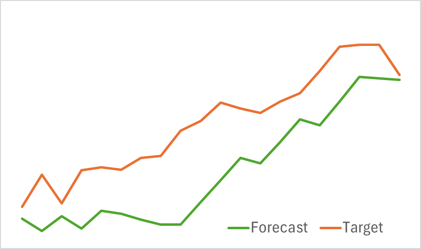
At the first stage, we train the Environmental State Encoder to forecast upcoming price movements. Training continues until the prediction error stabilizes at an acceptable level. Notably, we do not refresh or modify the training dataset during this phase. At this stage, the model demonstrated promising results. It showed a good ability to identify upcoming price trends.
In the second phase, we conduct iterative training of the Actor's behavioral policy and the Critic's reward function. The Critic model training serves a supporting role. It provided adjustments to the Actor's actions. However, our primary goal is to develop a profitable policy for the Actor. To ensure reliable evaluation of Actor's actions, we periodically update the training dataset during this phase. After several iterations, we successfully developed a policy capable of generating profits on the test dataset.
Let me remind you that all models are trained using historical data of the EURUSD symbol for 2023, H1 timeframe. Testing is performed on data from January 2024 while keeping all other parameters unchanged.
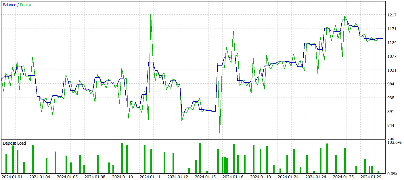
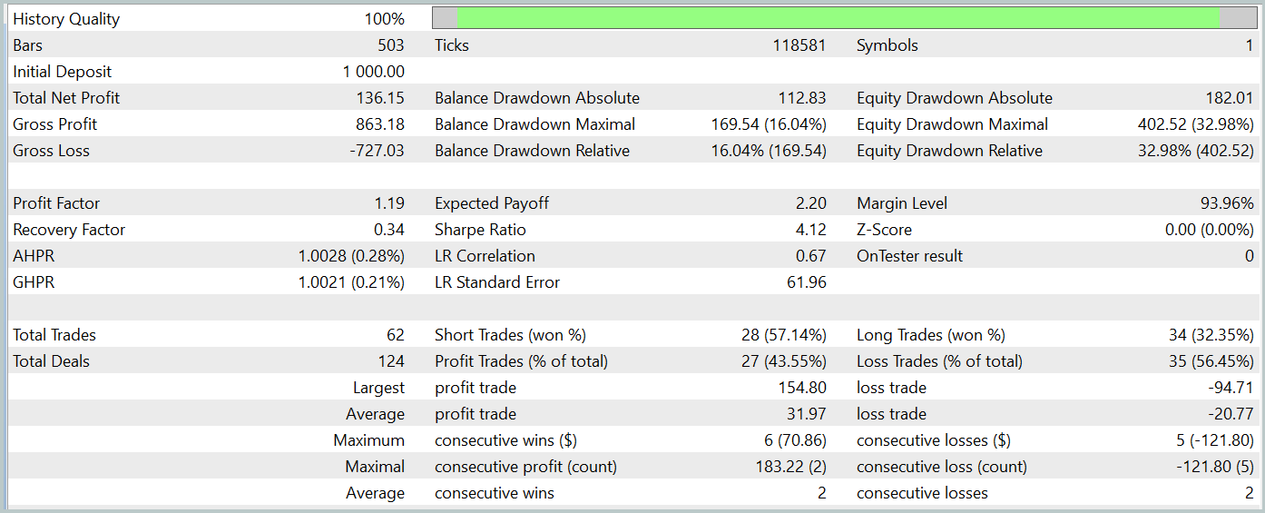
During the testing period, our model executed 62 trades and 27 of them (43.55%) were closed with a profit. However, due to the fact that the maximum and average profitable trades are more than half the same variables for losing trades, overall, a profit of 13.6% was obtained during the testing period. And the profit factor was at 1.19. However, a significant concern is the equity drawdown, which reached almost 33%. Clearly, in its current form, the model is not yet suitable for real-world trading and requires further improvements.
Conclusion
In this article, we explored the new Traj-LLM method, whose authors propose a novel perspective on applying large language models (LLMs). This method demonstrates how LLM capabilities can be adapted for forecasting future values of various time series, thus enabling more accurate and adaptive predictions under conditions of uncertainty and chaos.
In the practical section, we implemented our own interpretation of the proposed approach and tested it on real historical data. Although the results are not yet perfect, they are promising and indicate potential for further development.
References
- Traj-LLM: A New Exploration for Empowering Trajectory Prediction with Pre-trained Large Language Models
- Other articles from this series
Programs used in the article
| # | Issued to | Type | Description |
|---|---|---|---|
| 1 | Research.mq5 | EA | Example collection EA |
| 2 | ResearchRealORL.mq5 | EA | EA for collecting examples using the Real-ORL method |
| 3 | Study.mq5 | EA | Model training EA |
| 4 | StudyEncoder.mq5 | EA | Encoder training EA |
| 5 | Test.mq5 | EA | Model testing EA |
| 6 | Trajectory.mqh | Class library | System state description structure |
| 7 | NeuroNet.mqh | Class library | A library of classes for creating a neural network |
| 8 | NeuroNet.cl | Code Base | OpenCL program code library |
Translated from Russian by MetaQuotes Ltd.
Original article: https://www.mql5.com/ru/articles/15595
Warning: All rights to these materials are reserved by MetaQuotes Ltd. Copying or reprinting of these materials in whole or in part is prohibited.
This article was written by a user of the site and reflects their personal views. MetaQuotes Ltd is not responsible for the accuracy of the information presented, nor for any consequences resulting from the use of the solutions, strategies or recommendations described.

- Free trading apps
- Over 8,000 signals for copying
- Economic news for exploring financial markets
You agree to website policy and terms of use