Neural Networks in Trading: State Space Models

Introduction

In recent times, the paradigm of adapting large models to new tasks has become increasingly widespread. These models are pre-trained on extensive datasets containing arbitrary raw data from a broad spectrum of domains, including text, images, audio, time series, and more.

Although this concept is not tied to any specific architectural choice, most models are based on a single architecture – Transformer and its core layer Self-Attention. The efficiency of Self-Attention is attributed to its ability to densely direct information within a contextual window, enabling the modeling of complex data. However, this property has fundamental limitations: the inability to model anything beyond the finite window and the quadratic scaling with respect to the window length.

For sequence modeling tasks, an alternative solution involves using structured sequence models in state space (Space Sequence Models, SSM). These models can be interpreted as a combination of recurrent neural networks (RNNs) and convolutional neural networks (CNNs). This class of models can be computed very efficiently with linear or near-linear scaling of sequence length. Furthermore, it possesses inherent mechanisms for modeling long-range dependencies in specific data modalities.

One algorithm that enables the use of state space models for time series forecasting was introduced in the paper "Mamba: Linear-Time Sequence Modeling with Selective State Spaces". This paper presents a new class of selective state space models.

The authors identify a key limitation of existing models: the ability to effectively filter information based on input data (i.e., to focus on specific input data or ignore them). They develop a simple selection mechanism that makes SSM parameters dependent on input data. This allows the model to filter out irrelevant information and retain relevant information indefinitely.

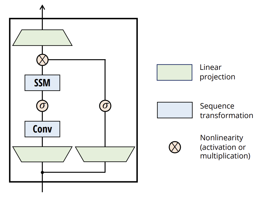
The authors simplify previous deep sequence model architectures by integrating the SSM architectural design with MLP into a single block, resulting in a simple and homogeneous architecture (Mamba) that incorporates selective state spaces.

Selective SSMs and, consequently, the Mamba architecture are fully recurrent models with key properties that make them suitable as the foundation for general-purpose sequence-based models.

1. High quality: Selectivity ensures high performance in dense modalities.
2. Fast training and inference: Computation and memory scale linearly with sequence length during training, while autoregressive model deployment during inference requires only constant time per step since it does not need to cache previous elements.
3. Long-term context: The combination of quality and efficiency enhances performance when handling large sequences.

1. Mamba Algorithm

The authors of Mamba argue that the fundamental challenge in sequence modeling is compressing context into a smaller state. The trade-offs of popular sequence models can be viewed from this perspective. For example, attention is simultaneously efficient and inefficient because it does not explicitly compress context at all. This is evident from the fact that autoregressive inference requires explicitly storing the entire context (i.e. the Key-Value cache), leading to slow linear-time inference and quadratic-time Transformer training.

Conversely, recurrent models are efficient because they maintain a finite state, implying constant-time inference and linear-time training. However, their efficiency is constrained by how well this state compresses the context.

To illustrate this principle, the authors focus on solving two synthetic tasks:

• Selective Copying Task. It requires content-aware reasoning to remember relevant tokens and filter out irrelevant ones.
• Induction Head Task. It explains most LLM capabilities in contextual learning. Solving this task requires context-dependent reasoning to determine when to retrieve the correct output in the appropriate context.

These tasks reveal failure modes in LTI models. From a recurrent perspective, their fixed dynamics prevent them from selecting the right information from their context or influencing the hidden state transmitted through the sequence based on input data. From a convolutional perspective, global convolutions can solve a vanilla copying task because it only requires awareness of time, but they struggle with selective copying due to a lack of content awareness. Specifically, the distance between inputs and outputs varies and cannot be modeled with static convolutional kernels.

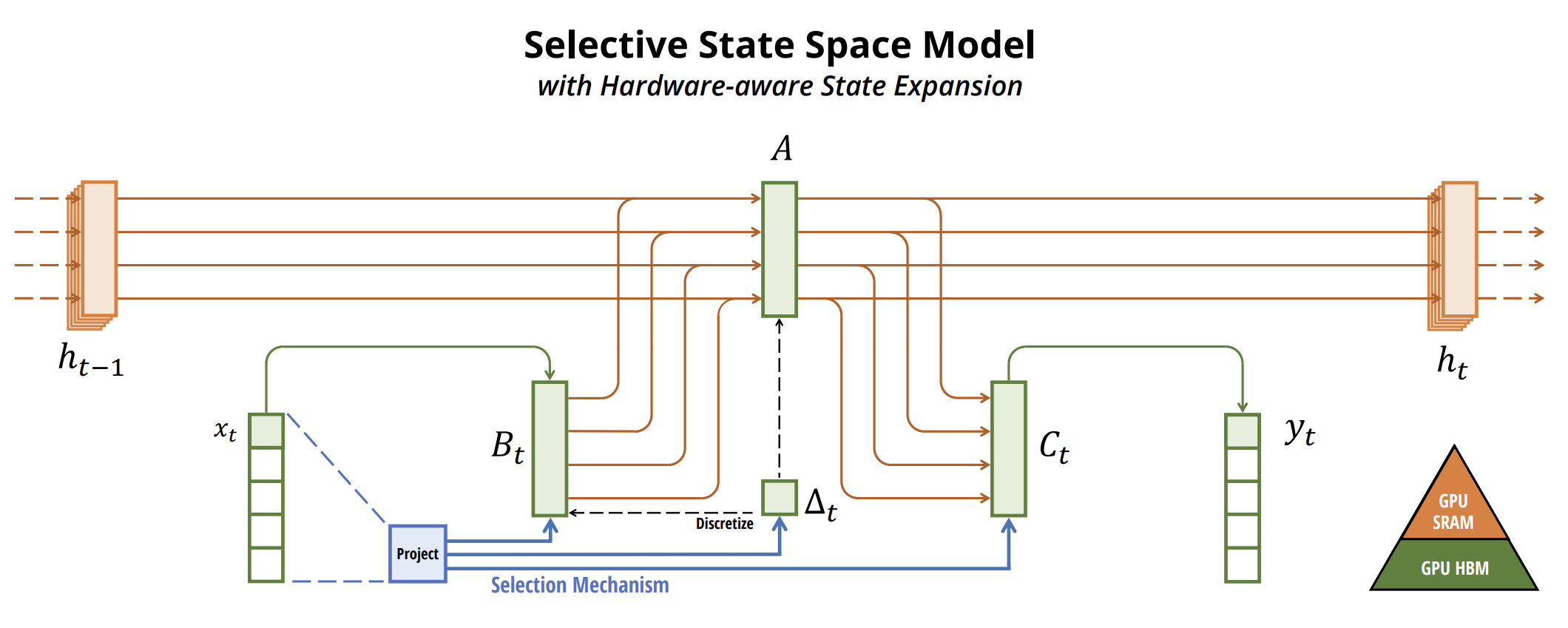
Thus, the efficiency trade-off in sequence models is characterized by how well they compress their state. In turn, the authors propose that the fundamental principle in designing sequence models is selectivity, or the context-dependent ability to focus on or filter out input data in sequential states. The selection mechanism controls how information propagates or interacts along the sequence dimension.

One method for incorporating selection mechanisms into models is to make parameters affecting sequence interactions dependent on input data. The key distinction is to simply make several parameters Δ B, C functions of the input data, along with corresponding changes in tensor shapes. Specifically, these parameters now have a length dimension L. This means the model transitions from being time-invariant to time-varying. 

The authors specifically choose:

• SB(x) = LinearN(x)
• SC(x) = LinearN(x)
• SΔ(x) = BroadcastD(Linear1(x))
• τΔ = SoftPlus

The choice of SΔ and τΔ is motivated by their connection to RNN gating mechanisms.

The authors aim to make selective SSMs efficient on modern hardware (GPUs). At a high level, recurrent models like SSMs always balance between efficiency and speed: models with higher hidden state dimensionality should be more efficient but slower. Thus, the challenge for Mamba was to maximize the hidden state dimension without sacrificing model speed or increasing memory consumption.

The selection mechanism overcomes limitations of LTI models. However, the computational challenge of SSMs remains. The authors address this with three classical techniques: kernel fusion, parallel scanning, and recomputation. They make two key observations:

• Naive recurrent computations use O(BLDN)FLOP, while convolutional computation requires O(BLD log(L)) FLOP. The former has a lower coefficient. Thus, for long sequences and not-too-large state dimensions N, the recurrent mode can actually use fewer FLOPs.
• The two main challenges are the sequential nature of recurrence and high memory usage. To address the latter, as with convolutional mode, they attempt to avoid computing the full state h.

The key idea is to leverage modern accelerators (GPUs) to compute h only at more efficient levels of the memory hierarchy. Most operations are memory bandwidth-bound, including scanning. The authors use kernel fusion to reduce memory I/O operations, significantly accelerating execution compared to a standard implementation.

Additionally, they carefully apply a classical recomputation technique to reduce memory requirements: intermediate states are not stored but recomputed in reverse during input processing.

Selective SSMs function as autonomous sequence transformations that can be flexibly embedded into neural networks.

The selection mechanism is a broader concept that can be applied differently to other parameters or through various transformations.

Selectivity allows us to remove irrelevant noise tokens that may occur among the relevant input data. An example of this is the selective copy problem, which occurs throughout common data modalities, especially for discrete data. This property arises because the model can mechanically filter out any specific input data Xt.

Empirical observations show that many sequence models do not improve with longer context, despite the principle that more context should strictly enhance performance. The explanation is that many sequence models cannot effectively ignore irrelevant context when necessary.

Conversely, selection models can reset their state at any moment to discard extraneous history, ensuring their performance improves monotonically with longer context.

The original visualization of the method is shown below.

2. Implementation in MQL5

After reviewing the theoretical aspects of the Mamba method, we move on to the practical implementation of the proposed approaches using MQL5. This work is divided into two stages. First, we construct the class implementing the SSM algorithm, which serves as one of the nested layers of the comprehensive Mamba method. Then, we build the top-level algorithmic processes.

2.1 SSM Implementation

There are numerous algorithms for constructing SSMs. For this experiment, I deviated slightly from the original Mamba implementation, creating one of the simplest state space selection models. This was implemented in the class CNeuronSSMOCL. As a parent object, we use the fully connected neural layer base class CNeuronBaseOCL. The structure of the new class is shown below.

class CNeuronSSMOCL  :  public CNeuronBaseOCL
  {
protected:
   uint              iWindowHidden;
   CNeuronBaseOCL    cHiddenStates;
   CNeuronConvOCL    cA;
   CNeuronConvOCL    cB;
   CNeuronBaseOCL    cAB;
   CNeuronConvOCL    cC;
   //---
   virtual bool      feedForward(CNeuronBaseOCL *NeuronOCL) override;
   //---
   virtual bool      calcInputGradients(CNeuronBaseOCL *NeuronOCL) override;
   virtual bool      updateInputWeights(CNeuronBaseOCL *NeuronOCL) override;
   //---

public:
                     CNeuronSSMOCL(void)  {};
                    ~CNeuronSSMOCL(void)  {};
   //---
   virtual bool      Init(uint numOutputs, uint myIndex, COpenCLMy *open_cl,
                          uint window, uint window_key, uint units_count, 
                          ENUM_OPTIMIZATION optimization_type, uint batch);
   //---
   virtual int       Type(void)   const   {  return defNeuronSSMOCL; }
   //---
   virtual bool      Save(int const file_handle);
   virtual bool      Load(int const file_handle);
   //---
   virtual bool      WeightsUpdate(CNeuronBaseOCL *source, float tau);
   virtual void      SetOpenCL(COpenCLMy *obj);
  };

In the presented structure, we see the declaration of one constant that defines the dimension of the hidden state of one element (iWindowHidden), and 5 internal neural layers. We will look at their functionality during the implementation.

The set of overridable methods in our class is quite standard. And I think you've already guessed their functional purpose.

All internal objects of the class are declared statically, which allows us to leave the class constructor and destructor empty. The initialization of all declared and inherited objects is carried out in the Init method. In the parameters of this method, we receive constants that allow us to clearly determine what object the user wanted to create.

bool CNeuronSSMOCL::Init(uint numOutputs, uint myIndex, COpenCLMy *open_cl, 
                         uint window, uint window_key, uint units_count, 
                         ENUM_OPTIMIZATION optimization_type, uint batch)
  {
   if(!CNeuronBaseOCL::Init(numOutputs, myIndex, open_cl, window * units_count, optimization_type, batch))
      return false;

There are 3 such parameters here:

• window – the vector size of one element in the sequence;
• window_key – size of the vector of internal representation of one element in the sequence;
• units_count – the size of the sequence being analyzed.

As I have already mentioned, in this experiment we are using a simplified SSM algorithm. In particular, it does not implement splitting a multimodal sequence into independent channels.

Within the method body, we immediately call the method of the same name from the parent class, which already contains the initialization of inherited objects and variables, as well as performing minimal and necessary validation of parameters received from the external program.

Once the parent class method has been successfully executed, we proceed to initialize the objects declared in this class. First, we initialize the internal layer responsible for storing the hidden state.

   if(!cHiddenStates.Init(0, 0, OpenCL, window_key * units_count, optimization, iBatch))
      return false;
   cHiddenStates.SetActivationFunction(None);
   iWindowHidden = window_key;

We also immediately store the size of the internal state vector of a single sequence element in a local variable.

It is important to note that we deliberately save this parameter value without performing any validation. The idea here is that we consciously initialized the internal layer first, whose size is determined by this parameter. If the user specifies an incorrect value, errors would occur during the class initialization stage itself. Thus, careful initialization of the internal layer implicitly performs parameter validation. This makes additional checks redundant at this stage.

It is also worth mentioning that the cHiddenStates object is used solely for temporary data storage, and we explicitly disable the activation function within it.

Next, we initialize two data projection layers that control how the input data influences the result. First, we initialize the hidden state projection layer:

   if(!cA.Init(0, 1, OpenCL, iWindowHidden, iWindowHidden, iWindowHidden, units_count, 1, optimization, iBatch))
      return false;
   cA.SetActivationFunction(SIGMOID);

Here, we use a convolutional layer, which allows us to perform independent projections of the hidden state for each sequence element. To regulate the influence of each element on the final result, we use a sigmoid as the activation function of this layer. As you know, the sigmoid function maps values into the range [0, 1]. With "0", the element does not influence the overall result.

We then initialize the input data projection layer in a similar way:

   if(!cB.Init(0, 2, OpenCL, window, window, iWindowHidden, units_count, 1, optimization, iBatch))
      return false;
   cB.SetActivationFunction(SIGMOID);

Note that both projection layers return tensors matching the size of the hidden state, even though their input tensors may have different dimensions. This is evident from the size of the data window and its step when initializing the objects.

To compute the combined influence of the input data and the hidden state on the result, we will use weighted summation. To optimize and reduce the number of operations, we decided to combine this step with the projection to the target result dimension. Therefore, we first concatenate the data into a common tensor along the sequence element dimension.

   if(!cAB.Init(0, 3, OpenCL, 2 * iWindowHidden * units_count, optimization, iBatch))
      return false;
   cAB.SetActivationFunction(None);

Next, we apply another internal convolutional layer.

   if(!cC.Init(0, 4, OpenCL, 2*iWindowHidden, 2*iWindowHidden, window, units_count, 1, optimization, iBatch))
      return false;
   cC.SetActivationFunction(None);

Finally, at the end of the initialization method, we redirect the pointers to the result and gradient buffers of our class to point to the equivalent buffers of the internal result projection layer. This simple step allows us to avoid unnecessary data copying during both forward and backward passes.

   SetActivationFunction(None);
   if(!SetOutput(cC.getOutput()) || !SetGradient(cC.getGradient()))
      return false;
//---
   return true;
  }

Naturally, we also monitor the success of all operations performed, and at the end of the method, we return a boolean value indicating success to the calling program.

After completing the initialization of the class, we move on to building the feed-forward pass algorithm. As you know, this functionality is implemented in the overridden feedForward method. Here everything is quite straightforward.

bool CNeuronSSMOCL::feedForward(CNeuronBaseOCL *NeuronOCL)
  {
   if(!cA.FeedForward(cHiddenStates.AsObject()))
      return false;
   if(!cB.FeedForward(NeuronOCL))
      return false;

The method parameters include a pointer to the preceding neural layer object, which provides the input data.

Inside the method, we immediately perform two projections (of the input data and the hidden state) to a compatible format. This is done using the forward pass methods of the corresponding internal convolutional layers.

The obtained projections are concatenated into a single tensor along the sequence element dimension.

   if(!Concat(cA.getOutput(), cB.getOutput(), cAB.getOutput(), iWindowHidden, iWindowHidden, 
                                                               cA.Neurons() / iWindowHidden))
      return false;

Finally, we project the concatenated layer to the required result dimension.

   if(!cC.FeedForward(cAB.AsObject()))
      return false;

There are two points to note here. First, we do not copy the result into the result buffer of the current layer – this operation is not needed since we redirect the data buffer pointers.

Second, you may have noticed that we did not update the hidden state. Thus, at this point, the forward pass method appears incomplete. However, the issue lies in the fact that we will still need the current hidden state for backpropagation purposes. Therefore, it makes sense to update the hidden state during the backpropagation pass, as it is only used within the algorithm of the current layer.

But there is a downside: during model inference (deployment), we do not use backpropagation methods. If we postpone the hidden state update to the backpropagation pass, it would never get updated during inference, violating the entire algorithm's logic.

Thus, we check the current operating mode of the model, and only during inference do we update the hidden state. We achieve this by summing and normalizing the projections of the previous hidden state and input data.

   if(!bTrain)
      if(!SumAndNormilize(cA.getOutput(), cB.getOutput(), cHiddenStates.getOutput(), iWindowHidden, true))
      return false;
//---
   return true;
  }

With this, our forward pass method becomes complete, and we return a boolean status of operation success to the calling program.

After implementing the feed-forward pass, we proceed to the backpropagation pass methods. As usual, we override two methods:

• calcInputGradients — for error gradient distribution.
• updateInputWeights — for model parameter updates.

The error gradient distribution algorithm mirrors the feed-forward pass in reverse order. I suggest you examine this method on your own - it is provided in the attached code. However, the parameter update method deserves special attention. Because we included the hidden state update process as part of model training.

bool CNeuronSSMOCL::updateInputWeights(CNeuronBaseOCL *NeuronOCL)
  {
   if(!cA.UpdateInputWeights(cHiddenStates.AsObject()))
      return false;
   if(!SumAndNormilize(cA.getOutput(), cB.getOutput(), cHiddenStates.getOutput(), iWindowHidden, true))
      return false;

Here, we first adjust the parameters of the internal hidden state projection layer. Only after that do we update the hidden state itself.

Notice that we do not check the model's operating mode here, as this method is only called during training.

Next, we call the corresponding parameter update methods of the remaining internal objects with learnable parameters.

   if(!cB.UpdateInputWeights(NeuronOCL))
      return false;
   if(!cC.UpdateInputWeights(cAB.AsObject()))
      return false;
//---
   return true;
  }

Upon completion of all operations, the method returns a boolean status to the calling program.

This concludes the discussion of the SSM implementation class methods. You can find the full code of all these methods in the attachment.

2.2 Mamba Method Class

We have implemented the class for the SSM layer. Now, we can move on to building the top-level algorithm of the Mamba method. To implement the method, we will create a class CNeuronMambaOCL, which, like the previous one, will inherit base functionality from the fully connected layer class CNeuronBaseOCL. The structure of the new class is shown below.

class CNeuronMambaOCL   :  public CNeuronBaseOCL
  {
protected:
   CNeuronConvOCL    cXProject;
   CNeuronConvOCL    cZProject;
   CNeuronConvOCL    cInsideConv;
   CNeuronSSMOCL     cSSM;
   CNeuronBaseOCL    cZSSM;
   CNeuronConvOCL    cOutProject;
   CBufferFloat      Temp;
   //---
   virtual bool      feedForward(CNeuronBaseOCL *NeuronOCL) override;
   //---
   virtual bool      calcInputGradients(CNeuronBaseOCL *NeuronOCL) override;
   virtual bool      updateInputWeights(CNeuronBaseOCL *NeuronOCL) override;
   //---

public:
                     CNeuronMambaOCL(void) {};
                    ~CNeuronMambaOCL(void) {};
   //---
   virtual bool      Init(uint numOutputs, uint myIndex, COpenCLMy *open_cl, 
                          uint window, uint window_key, uint units_count, 
                          ENUM_OPTIMIZATION optimization_type, uint batch);
   //---
   virtual int       Type(void)   const   {  return defNeuronMambaOCL; }
   //---
   virtual bool      Save(int const file_handle);
   virtual bool      Load(int const file_handle);
   //---
   virtual bool      WeightsUpdate(CNeuronBaseOCL *source, float tau);
   virtual void      SetOpenCL(COpenCLMy *obj);
  };

Here, we can see a familiar set of overridable methods and the declaration of internal neural network layers, whose functionalities we will explore during the implementation of class methods.

At the same time, there are no internal variables declared to store constants. We will discuss the decisions that allowed us to avoid saving constants during the implementation phase.

As usual, all internal objects are declared statically. Therefore, both the constructor and destructor of the class remain empty. The initialization of objects is performed in the Init method.

bool CNeuronMambaOCL::Init(uint numOutputs, uint myIndex, COpenCLMy *open_cl, 
                           uint window, uint window_key, uint units_count, 
                           ENUM_OPTIMIZATION optimization_type, uint batch)
  {
   if(!CNeuronBaseOCL::Init(numOutputs, myIndex, open_cl, window * units_count, optimization_type, batch))
      return false;

A list of parameters in this method is similar to the method of the same name in the previously discussed CNeuronSSMOCL class. It is not difficult to guess that they have similar functions.

In the method body, we first call the parent class initialization method, which handles inherited objects and variables.

As you may recall from the theoretical explanation of the Mamba method, the input data here follows two parallel streams. For both streams, we perform data projections that will be executed using convolutional layers.

   if(!cXProject.Init(0, 0, OpenCL, window, window, window_key + 2, units_count, 1, optimization, iBatch))
      return false;
   cXProject.SetActivationFunction(None);
   if(!cZProject.Init(0, 1, OpenCL, window, window, window_key, units_count, 1, optimization, iBatch))
      return false;
   cZProject.SetActivationFunction(SIGMOID);

In the first stream, we use a convolutional layer and an SSM block. In the second, we apply an activation function, after which the data proceeds to the merging stage. Consequently, the outputs of both streams must be tensors of comparable size. To achieve this, we slightly increase the projection size of the first stream, which is compensated for by data compression during convolution.

Note that the activation function is used only for the projection of the second stream.

The next step is initializing the convolutional layer.

   if(!cInsideConv.Init(0, 2, OpenCL, 3, 1, 1, window_key, units_count, optimization, iBatch))
      return false;
   cInsideConv.SetActivationFunction(SIGMOID);

Here, we perform independent convolution within individual sequence elements. Therefore, we specify the size of the hidden state tensor as the number of convolution elements. We also add the number of sequence elements as independent variables.

The convolution window size and stride align with our increased projection size for the first data stream.

At this point, we also add an activation function to ensure the comparability of data across both streams.

Next comes our SSM block, which performs state selection.

   if(!cSSM.Init(0, 3, OpenCL, window_key, window_key, units_count, optimization, iBatch))
      return false;

To complete the algorithm and introduce non-linearity to the merging of the two data streams, we concatenate the outputs into a unified tensor.

   if(!cZSSM.Init(0, 4, OpenCL, 2 * window_key * units_count, optimization, iBatch))
      return false;
   cZSSM.SetActivationFunction(None);

We then project the resulting data to the required size within each sequence element using another convolutional layer.

   if(!cOutProject.Init(0, 5, OpenCL, 2*window_key, 2*window_key, window, units_count, 1, optimization, iBatch))
      return false;
   cOutProject.SetActivationFunction(None);

Additionally, we allocate a buffer to store intermediate results.

   if(!Temp.BufferInit(window * units_count, 0))
      return false;
   if(!Temp.BufferCreate(OpenCL))
      return false;

And we perform pointer swapping to reference these buffers.

   if(!SetOutput(cOutProject.getOutput()))
      return false;
   if(!SetGradient(cOutProject.getGradient()))
      return false;
   SetActivationFunction(None);
//---
   return true;
  }

Finally, the method returns a boolean result of the performed operations to the calling program.

After completing the class initialization method, we move on to implementing the feed-forward algorithm in the feedForward method. A part of this algorithm was already mentioned during the initialization method's creation. Now let's look at its implementation in code.

bool CNeuronMambaOCL::feedForward(CNeuronBaseOCL *NeuronOCL)
  {
   if(!cXProject.FeedForward(NeuronOCL))
      return false;
   if(!cZProject.FeedForward(NeuronOCL))
      return false;

The method receives a pointer to the previous layer's object, whose buffer contains our input data. Within the method body, we immediately project the incoming data by calling the forward pass methods of our projection convolutional layers.

At this point, we complete the operations of the second information stream. However, we still need to process the main data stream. Here, we start with data convolution.

   if(!cInsideConv.FeedForward(cXProject.AsObject()))
      return false;

After which we perform state selection.

   if(!cSSM.FeedForward(cInsideConv.AsObject()))
      return false;

Once both streams' operations are finished, we merge the results into a unified tensor.

   if(!Concat(cSSM.getOutput(), cZProject.getOutput(), cZSSM.getOutput(), 1, 1, cSSM.Neurons()))
      return false;

It is important to note that we did not store the dimension of an individual sequence element's internal state. That is not a problem. We know that the tensors from both information streams are of equal dimensions. Therefore, we can sequentially combine one element from each tensor without disrupting the overall structure.

Finally, we project the data to the desired output dimension.

   if(!cOutProject.FeedForward(cZSSM.AsObject()))
      return false;
//---
   return true;
  }

The method concludes by returning a boolean result to the calling program, indicating the success of operations.

As you can see, the feed-forward pass algorithm is not particularly complex. The same applies to the backpropagation pass methods. Therefore, we will not consider in detail their algorithms within this article. The complete code of this class and all its methods is included in the attached files.

2.3 Model Architecture

In the previous sections, we implemented our interpretation of the approaches proposed by the Mamba authors. However, the work done should produce results. To evaluate the efficiency of the implemented algorithms, we need to integrate them into our model. You might have already guessed that we will add the newly created layers to the Environment State Encoder model. After all, this is the model we train within the framework of predicting future price movements.

The architecture of this model is presented in the CreateEncoderDescriptions method.

bool CreateEncoderDescriptions(CArrayObj *&encoder)
  {
//---
   CLayerDescription *descr;
//---
   if(!encoder)
     {
      encoder = new CArrayObj();
      if(!encoder)
         return false;
     }

The method receives a pointer to a dynamic array, into which we will write the architecture description of the model being created.

In the method body, we check the relevance of the received pointer and, if necessary, create a new instance of the object. After this preparatory step, we proceed to describe the model architecture.

The first layer is intended for inputting raw data into the model. As usual, we use a fully connected layer of sufficient size.

//--- Encoder
   encoder.Clear();
//--- Input layer
   if(!(descr = new CLayerDescription()))
      return false;
   descr.type = defNeuronBaseOCL;
   int prev_count = descr.count = (HistoryBars * BarDescr);
   descr.activation = None;
   descr.optimization = ADAM;
   if(!encoder.Add(descr))
     {
      delete descr;
      return false;
     }

Usually we input "raw" initial data to the model in the form in which we receive it from the terminal. Naturally, these inputs belong to different distributions. We know that any model's efficiency improves significantly when working with normalized and comparable values. Therefore, to bring the diverse input data to a comparable scale, we use a batch normalization layer.

//--- layer 1
   if(!(descr = new CLayerDescription()))
      return false;
   descr.type = defNeuronBatchNormOCL;
   descr.count = prev_count;
   descr.batch = 1e4;
   descr.activation = None;
   descr.optimization = ADAM;
   if(!encoder.Add(descr))
     {
      delete descr;
      return false;
     }

Next, we create a block of three identical Mamba layers. For this, we define a single architecture description for the block and add it to the array the required number of times.

   if(!(descr = new CLayerDescription()))
      return false;
   descr.type = defNeuronMambaOCL;
   descr.window = BarDescr;                                       //window
   descr.window_out = 4 * BarDescr;                               //Inside Dimension
   prev_count = descr.count = HistoryBars;                        //Units
   descr.batch = 1e4;
   descr.activation = None;
   descr.optimization = ADAM;
   for(int i = 2; i <= 4; i++)
      if(!encoder.Add(descr))
        {
         delete descr;
         return false;
        }

Note that the size of the analyzed data window corresponds to the number of elements describing a single sequence element, and the size of the internal representation is four times larger. This follows the authors' recommendation to perform an expanding projection in the Mamba method.

The number of sequence elements corresponds to the depth of the analyzed history.

As I mentioned during the class implementation, in this version we did not allocate separate information channels. Nevertheless, our algorithm processes independent sequence elements. If you need to analyze independent channels, you can pre-transpose the data and adjust the layer parameters accordingly. But this is a topic for another experiment.

However, we will predict sequences across independent channels. Therefore, after the Mamba block, we transpose the data.

//--- layer 5
   if(!(descr = new CLayerDescription()))
      return false;
   descr.type = defNeuronTransposeOCL;
   descr.count = prev_count;
   descr.window = BarDescr;
   descr.activation = None;
   descr.optimization = ADAM;
   if(!encoder.Add(descr))
     {
      delete descr;
      return false;
     }

We then apply two convolutional layers to forecast the next values for the independent channels.

//--- layer 6
   if(!(descr = new CLayerDescription()))
      return false;
   descr.type = defNeuronConvOCL;
   descr.count = BarDescr;
   descr.window = prev_count;
   descr.window_out = 4 * NForecast;
   descr.activation = LReLU;
   descr.optimization = ADAM;
   if(!encoder.Add(descr))
     {
      delete descr;
      return false;
     }
//--- layer 7
   if(!(descr = new CLayerDescription()))
      return false;
   descr.type = defNeuronConvOCL;
   descr.count = BarDescr;
   descr.window = 4 * NForecast;
   descr.window_out = NForecast;
   descr.activation = TANH;
   descr.optimization = ADAM;
   if(!encoder.Add(descr))
     {
      delete descr;
      return false;
     }

After that, we return the predicted values to their original representation.

//--- layer 8
   if(!(descr = new CLayerDescription()))
      return false;
   descr.type = defNeuronTransposeOCL;
   descr.count = BarDescr;
   descr.window = NForecast;
   descr.activation = None;
   descr.optimization = ADAM;
   if(!encoder.Add(descr))
     {
      delete descr;
      return false;
     }

Additionally, we append statistical characteristics of the original data distribution, obtained during normalization.

//--- layer 9
   if(!(descr = new CLayerDescription()))
      return false;
   descr.type = defNeuronRevInDenormOCL;
   descr.count = BarDescr * NForecast;
   descr.activation = None;
   descr.optimization = ADAM;
   descr.layers = 1;
   if(!encoder.Add(descr))
     {
      delete descr;
      return false;
     }

The final step of our model is adjusting the results in the frequency domain.

//--- layer 10
   if(!(descr = new CLayerDescription()))
      return false;
   descr.type = defNeuronFreDFOCL;
   descr.window = BarDescr;
   descr.count =  NForecast;
   descr.step = int(true);
   descr.probability = 0.7f;
   descr.activation = None;
   descr.optimization = ADAM;
   if(!encoder.Add(descr))
     {
      delete descr;
      return false;
     }
//---
   return true;
  }

The architectures of the Actor and Critic models remain unchanged. Also, programs for interaction with the environment did not require modifications. However, we did have to introduce some targeted changes in the model training programs. This is because using the hidden state within the SSM block requires adjusting the sequence of input data in a manner characteristic of recurrent models. Such adjustments are standard whenever models with hidden states are used, where information accumulates over time. I encourage you to study them in the attachment. The complete code for all programs and classes used in preparing this article is included there. With this, we conclude the description of the implementation and move on to practical testing on real historical data.

3. Testing

Our work is nearing completion, and we are moving to the final stage – training the models and testing the achieved results. The models are trained on historical EURUSD data for 2023 with an H1 timeframe. The parameters of all indicators are set to default.

In the first stage, we train the Environment State Encoder to forecast future price movements over a specified time horizon. This model analyzes only historical price data, fully ignoring Actor's actions. This allows us to conduct comprehensive model training using previously collected datasets without needing to update them. However, such updates may be necessary if the historical training period is changed or extended.

The first observation is that the model turned out to be compact and fast. The training process was relatively stable and robust. The model showed interesting results.

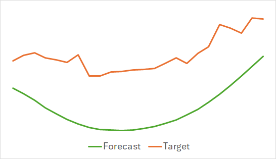
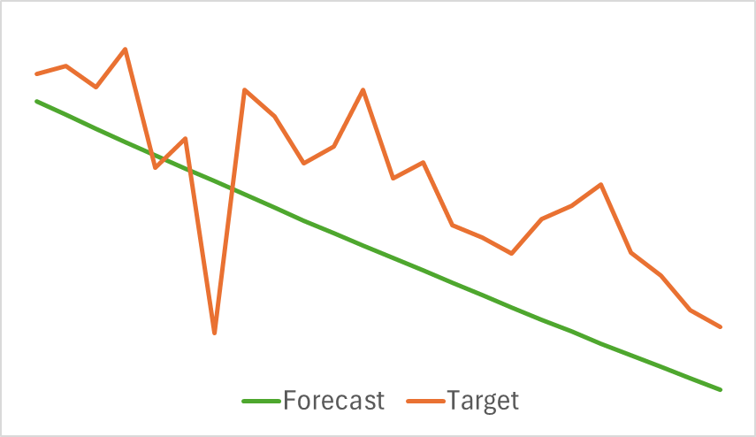
The above graphs display the predicted price movements for the next 24 hours. Notably, in the first graph the forecast line smoothly indicates a trend change, while in the second case, it almost linearly reflects the ongoing trend.

In the second stage, we performed iterative Actor policy training. We also trained the Critic value function. The Critic's role is to guide the Actor in improving its policy efficiency.

As mentioned earlier, the second training phase is iterative. This means that throughout the training, we periodically update the training dataset to include data relevant to the current Actor policy. Maintaining an up-to-date training set is crucial for proper model training.

However, during the training process, we did not achieve a policy with a clearly defined deposit growth trend. Although the model managed to generate profit on the historical test data for January 2024, no consistent trend was observed.

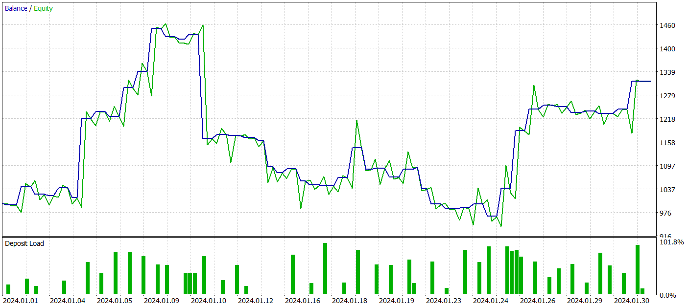
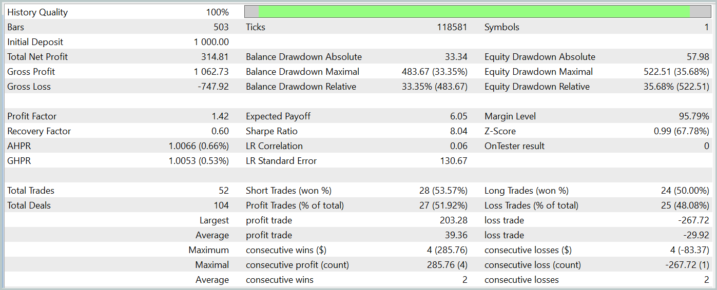
During the test period, the model executed 52 trades, of which 27 closed with a profit, i.e. nearly 52%. The average profit exceeded the average loss per trade (39.36 vs. -29.82). Nevertheless, the maximum loss was 30% greater than the maximum profit. Additionally, we observed a drawdown of more than 35% in equity. Clearly, this model requires further refinement.

The profit and loss breakdown by hours and days is also interesting.

Fridays stand out as notably profitable, while Wednesdays show losses. There are also specific intraday periods with clusters of profitable and losing trades. This needs further analysis. Particularly since the average position holding time was slightly over an hour, with a maximum of two hours.

Conclusion

In this article, we discussed a new time series forecasting method Mamba, which offers an efficient alternative to traditional architectures such as the Transformer. By integrating sample state space models (SSM), Mamba provides high throughput and linear scaling in sequence length.

In the practical part of our article, we implemented our vision of the proposed approaches using MQL5. We trained models on real-world data and got mixed results.

References

• Mamba: Linear-Time Sequence Modeling with Selective State Spaces
• Other articles from this series

Programs used in the article

#	Issued to	Type	Description
1	Research.mq5	EA	Example collection EA
2	ResearchRealORL.mq5	EA	EA for collecting examples using the Real-ORL method
3	Study.mq5	EA	Model training EA
4	StudyEncoder.mq5	EA	Encoder training EA
5	Test.mq5	EA	Model testing EA
6	Trajectory.mqh	Class library	System state description structure
7	NeuroNet.mqh	Class library	A library of classes for creating a neural network
8	NeuroNet.cl	Code Base	OpenCL program code library