
Neural Networks in Trading: Lightweight Models for Time Series Forecasting

Introduction
Forecasting future price movements is crucial for developing an effective trading strategy. Achieving accurate forecasts typically requires the use of powerful and complex deep learning models.
The foundation of precise long-term time series forecasting lies in the inherent periodicity and trends present in the data. Additionally, it has long been observed that the price movements of currency pairs are closely related to specific trading sessions. For instance, if a time series of daily sequences is discretized at a specific time of day, each subsequence exhibits similar or sequential trends. In this case, the periodicity and trend of the original sequence are decomposed and transformed. Periodic patterns are converted into inter-subsequence dynamics, while trend patterns are reinterpreted as intra-subsequence characteristics. This decomposition opens new avenues for developing lightweight models for long-term time series forecasting, an approach explored in the paper "SparseTSF: Modeling Long-term Time Series Forecasting with 1k Parameters".
In their work, the authors investigate, perhaps for the first time, how periodicity and data decomposition can be leveraged to build specialized lightweight time series forecasting models. This approach enables them to propose SparseTSF, an extremely lightweight model for long-term time series forecasting.
The authors present a technical method for inter-period sparse forecasting. First, the input data is divided into constant-periodicity sequences. Then prediction is performed for each downsampled subsequence. Thus, the original problem of forecasting time series is simplified to the problem of forecasting the interperiod trend.
This approach offers two advantages:
- Efficient separation of data periodicity and trend, allowing the model to stably identify and capture periodic features while focusing on predicting trend changes.
- Extreme compression of the model parameters size, significantly reducing the requirements for computing resources.
1. The SparseSTF Algorithm
The objective of long-term time series forecasting (LTSF) is to predict future values over an extended horizon using previously observed multivariate time series data. The primary goal of LTSF is to extend the forecasting horizon H, as this provides more comprehensive and advanced insights for practical applications. However, extending the forecasting horizon often increases the complexity of the trained model. To address this issue, the authors of SparseTSF focused on developing models that are not only exceptionally lightweight but also robust and efficient.
Recent advancements in LTSF have led to a shift toward independent channel forecasting when dealing with multivariate time series data. This strategy simplifies the forecasting process by focusing on individual univariate time series within the dataset, reducing the complexity of inter-channel dependencies. As a result, the primary focus of contemporary models in recent years has shifted toward efficient forecasting by modeling long-term dependencies, including periodicity and trends, in univariate sequences.
Given that forecasted data often exhibit consistent, a priori periodicity, the authors of SparseTSF propose inter-period sparse forecasting to enhance the extraction of long-term sequential dependencies while simultaneously reducing model parameter complexity. The proposed solution utilizes a single linear layer to model the LTSF task.
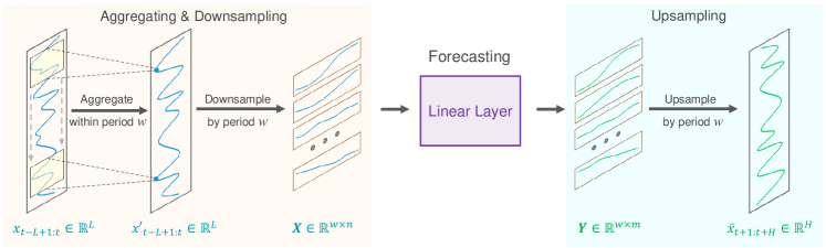
It is assumed that a time series Xt of length L has a known periodicity w. The first step of the proposed algorithm is to downsample the original sequence into w subsequences of length n (n=L/w). A forecasting model with shared parameters is then applied to these subsequences. This operation results in w predicted subsequences, each of length m (m=H/w), which together form the complete predicted sequence of length H.
Intuitively, this forecasting process resembles a sliding forecast with a sparse interval w, performed by a fully connected layer with parameter sharing over a fixed period w. This can be interpreted as a model performing sparse sliding forecasting over periods.
From a technical perspective, the downsampling process is equivalent to reshaping the tensor of the original data Xt into an n*w matrix, followed by transposition into a w*n matrix. Sparse sliding trajectory forecasting is then equivalent to applying a linear layer of size n*m to the final dimension of the matrix. The operation results in a w*m matrix.
During upsampling, we perform the inverse operations: transposing the w*m matrix and then reformatting it into the full predicted sequence of length H.
However, the proposed approach faces two problems:
- Loss of information, as only one data point per period is used for forecasting while others are ignored.
- Increased sensitivity to outliers, as extreme values within downsampled subsequences can directly impact the forecast.
To mitigate these issues, the authors of SparseTSF introduce a sliding aggregation step before performing sparse forecasting. Each aggregated data point incorporates information from surrounding points within the period, addressing the first issue. Moreover, since the aggregated value essentially represents a weighted average of surrounding points, it mitigates the impact of outliers, thereby resolving the second issue.
Technically, this sliding data aggregation can be implemented using a convolutional layer with zero padding.
Time series data often exhibit distribution shifts between training and testing datasets. Simple normalization strategies between the original data and predicted sequences can help mitigate this issue. In the SparseTSF algorithm, a straightforward normalization strategy is employed: the mean value of the sequence is subtracted from the input data before being fed into the model and is then added back to the resulting forecasts.
Authors' visualization of the SparseTSF method is presented below.
2. Implementing in MQL5
After considering the theoretical aspects of the SparseTSF method, let's move on to implementing the proposed approaches using MQL5. As part of our library, we will create a new class, CNeuronSparseTSF.
2.1 Creating the SparseTSF class
Our new class will inherit the core functionality from the base class CNeuronBaseOCL. The structure of the CNeuronSparseTSF class is shown below.
class CNeuronSparseTSF  :  public CNeuronBaseOCL
  {
protected:
   CNeuronConvOCL       cConvolution;
   CNeuronTransposeOCL  acTranspose[4];
   CNeuronConvOCL       cForecast;
   //---
   virtual bool      feedForward(CNeuronBaseOCL *NeuronOCL) override;
   //---
   virtual bool      calcInputGradients(CNeuronBaseOCL *NeuronOCL) override;
   virtual bool      updateInputWeights(CNeuronBaseOCL *NeuronOCL) override;

public:
                     CNeuronSparseTSF(void) {};
                    ~CNeuronSparseTSF(void) {};
   //---
   virtual bool      Init(uint numOutputs, uint myIndex, COpenCLMy *open_cl,
                          uint sequence, uint variables, uint period, uint forecast,
                          ENUM_OPTIMIZATION optimization_type, uint batch);
   //---
   virtual int       Type(void)   const   {  return defNeuronSparseTSF;   }
   //---
   virtual bool      Save(int const file_handle);
   virtual bool      Load(int const file_handle);
   //---
   virtual bool      WeightsUpdate(CNeuronBaseOCL *source, float tau);
   virtual void      SetOpenCL(COpenCLMy *obj);
  };
In the structure of the new class, we will add 2 convolutional layers. One of them performs the role of data aggregation, and the second one predicts subsequent sequences. In addition, we will use a whole array of transpositions to reformat the data. All added internal objects are declared statically, which allows the class constructor and destructor to remain "empty". Initialization of a class object is performed in the Init method.
In the parameters of the initialization method, we pass the main parameters of the created object:
- sequence — length of the sequence of initial data
- variables — the number of univariate sequences within the analyzed multimodal time series
- period — periodicity of input data
- forecast — depth of forecast.
bool CNeuronSparseTSF::Init(uint numOutputs, uint myIndex, COpenCLMy *open_cl,
                            uint sequence, uint variables,
                            uint period, uint forecast,
                            ENUM_OPTIMIZATION optimization_type, uint batch
                           )
  {
   if(!CNeuronBaseOCL::Init(numOutputs, myIndex, open_cl, forecast * variables, optimization_type, batch))
      return false;
In the body of the method, as usual, we call the parent class method having the same name. This method already implements the process of initializing inherited objects and variables.
Note that when calling the initialization method of the parent class, we specify the layer size equal to the product of the forecasting depth and the number of unitary sequences in the multimodal data.
After successful initialization of inherited objects and variables, we move on to the stage of initialization of added internal objects. We will initialize them in the sequence of the feed-forward pass. Now, pay special attention to the dimension of the data tensor we are processing.
At the input of the layer we expect to receive an input data tensor of dimension L*v, where L is the length of the input sequence andv is the number of unitary series in multimodal source data. As was said in the first part of this article, the SparseTSF method works in the paradigm of predicting independent unitary sequences. To implement such a process, we transpose the input data matrix into a v*L matrix.
   if(!acTranspose[0].Init(0, 0, OpenCL, sequence, variables, optimization, iBatch))
      return false;
Next, we plan to aggregate the input data using a convolutional layer. In this operation, we will perform a convolution within 2 periods of the original data with a step of 1 period. To preserve dimensionality, the number of convolution filters is equal to the period size.
   if(!cConvolution.Init(0, 1, OpenCL, 2 * period, period, period, sequence / period, variables, optimization, iBatch))
      return false;
   cConvolution.SetActivationFunction(None);
Please note that we perform data aggregation within independent unitary sequences.
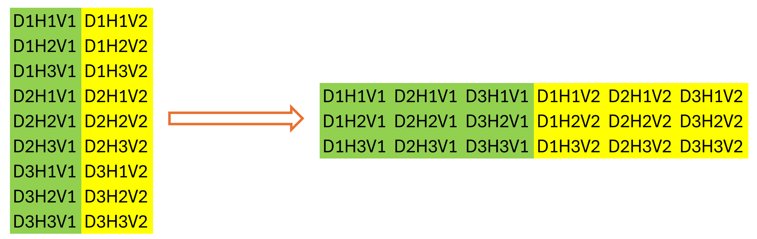
The next step of the SparseTSF algorithm is the discretization of the original data. At this stage, the authors of the method suggest changing the dimensionality and transposing the tensor of the original data. In our case, we are working with one-dimensional data buffers. Changing the dimensionality of the original data is purely declarative; it does not involve rearranging the data in memory. However, the same cannot be said for transposition. Therefore, we proceed by initializing the next layer for data transposition.
   if(!acTranspose[1].Init(0, 2, OpenCL, variables * sequence / period, period, optimization, iBatch))
      return false;
It may seem a little strange to use a second data transposition layer. At first glance, it performs an operation that is the inverse of the previous transposition of the original data. But that;s not quite true. It have emphasized the dimensions of the data above. The total size of our data buffer remains unchanged: L*v. Only after declaratively changing the dimension of the data matrix we can say that its size is equal to (v * L/w) * w, where w is periodicity of the initial data. We transpose it into w * (L/w * v). After this operation, our data buffer will display a sequence of individual stages of periodicity of the original data, taking into account the independence of the unitary series of the original data.
Graphically, the result of the two stages of data transposition can be represented as follows:
We then use a convolutional layer to independently predict individual steps within the periodicity of the input data for unitary sequences over a given planning horizon.
   if(!cForecast.Init(0, 3, OpenCL, sequence / period, sequence / period, forecast / period,
                                                       variables, period, optimization, iBatch))
      return false;
   cForecast.SetActivationFunction(TANH);
Note that the size of the analyzed source data window and its step is "sequence / period", and the number of convolution filters is "forecast / period". This allows us to obtain forecast values for the entire planning horizon in one pass. In this case, we use separate filters for each step of the period of the analyzed data.
Since we intend to work with normalized data, we use the hyperbolic tangent as the activation function for the predicted values. This allows us to limit the forecast results to the range [-1, 1].
Next, we need to convert the predicted values into the required sequence. We perform this operation using two successive layers of data transposition, which perform the inverse permutation operations of the values.
   if(!acTranspose[2].Init(0, 4, OpenCL, period, variables * forecast / period, optimization, iBatch))
      return false;
   if(!acTranspose[3].Init(0, 5, OpenCL, variables, forecast, optimization, iBatch))
      return false;
In order to avoid unnecessary copying of data, we organize the substitution of the result buffers and error gradients of the current layer.
   if(!SetOutput(acTranspose[3].getOutput()) ||
      !SetGradient(acTranspose[3].getGradient())
     )
      return false;
//---
   return true;
  }
At each iteration, we check the results of the operations. The final logical result of the method's operation is the returned to the caller.
Please note that during the object initialization process, we did not save the architecture parameters of the layer we are creating. In this case, we just need to pass the appropriate parameters to the nested objects. Their architecture uniquely defines the operation of the class, so there is no need to additionally store the received parameters.
After initializing the class object, we move on to creating the feed-forward method CNeuronSparseTSF::feedForward, in which we construct the algorithm of the SparseTSF method with data transfer between internal objects.
In the parameters of the feed-forward method, we receive a pointer to the object of the previous layer, which contains the original data.
bool CNeuronSparseTSF::feedForward(CNeuronBaseOCL *NeuronOCL)
  {
   if(!acTranspose[0].FeedForward(NeuronOCL))
      return false;
Since we will recreate the algorithm using previously created methods of nested objects, we do not add the validation of the received pointer. We simply pass it to the feed-forward method of the first data transposition layer, in which a similar check is already implemented along with the operations of the main functionality related to data permutation in the data buffer. We only check the logical result of executing the operations of the called method.
Next, we perform data aggregation by calling the feed-forward method of the convolutional layer.
   if(!cConvolution.FeedForward(acTranspose[0].AsObject()))
      return false;
In accordance with the SparseTSF algorithm, the aggregated data is summed with the original data. However, to maintain the consistency of the data, we will sum the transposed version of the original data with the aggregation results.
   if(!SumAndNormilize(cConvolution.getOutput(), acTranspose[0].getOutput(), cConvolution.getOutput(), 1, false))
      return false;
In the next step, we call the feed-forward method of the next data transposition layer, which completes the discretization process of the original sequence.
   if(!acTranspose[1].FeedForward(cConvolution.AsObject()))
      return false;
After that, we forecast the most probable continuation of the analyzed time series using the second nested convolutional layer.
   if(!cForecast.FeedForward(acTranspose[1].AsObject()))
      return false;
Let me remind you that the forecasting of subsequences is carried out on the basis of the analysis of individual steps within the given periodicity of the initial data. In this case, we make independent forecasts for each unitary sequence of the multimodal input time series. For each step of the closed cycle of the input data periodicity, we use individual training parameters.
The rearrangement of predicted values into the required order of the expected output sequence is carried out using two consecutive layers of data transposition.
   if(!acTranspose[2].FeedForward(cForecast.AsObject()))
      return false;
   if(!acTranspose[3].FeedForward(acTranspose[2].AsObject()))
      return false;
//---
   return true;
  }
Of course, for the step of reordering predicted values in the data buffer, we could create a new kernel and replace the two transposition layers with a single kernel call. This would provide some performance improvement by eliminating unnecessary data transfer operations. However, given the size of the model, the expected performance gain is negligible. In this experiment, we opted to simplify the program code and reduce the programmer's workload.
It is important to note that the operations of the forward pass method conclude with the execution of the feed-forward pass methods of nested objects. At the same time, we do not transfer values to the result buffer of the current layer, which is inherited from the parent class. However, subsequent layers of our model do not have access to nested objects and operate on the result buffer of our layer. To compensate for this apparent data flow gap, we substituted the result and error gradient buffers during the initialization of our class. As a result, the result buffer of our layer received a pointer to the result buffer of the last transposition layer. Thus, by performing the final transposition operation, we effectively write data into our layer's result buffer, eliminating unnecessary data transfer operations between objects.
As always, at each stage, we verify the outcome of the operations and return the final logical result to the calling program.
With this, we complete the implementation of the feed-forward pass of the SparseTSF method and proceed to constructing the backpropagation algorithms. Here, we need to distribute the error gradient among all participants in the process according to their influence on the result and adjust the model parameters to minimize the forecasting error of the analyzed multimodal time series.
The first step is to develop the method for distributing the error gradient: CNeuronSparseTSF::calcInputGradients. As with the feed-forward pass, the method parameters include a pointer to the previous layer's object, where we will record the error gradient based on the influence of the original data on the model output.
bool CNeuronSparseTSF::calcInputGradients(CNeuronBaseOCL *NeuronOCL)
  {
   if(!acTranspose[2].calcHiddenGradients(acTranspose[3].AsObject()))
      return false;
We will distribute the error gradient according to the feed-forward operations but in reverse order. As you know, due to pointer substitution for data buffers, the error gradient received from the next model layer ends up in the buffer of the last internal transposition layer. This allows us to proceed with internal objects directly, without additional data transfer operations.
First, we pass the error gradient through the two transposition layers to achieve the required discretization of gradients.
   if(!cForecast.calcHiddenGradients(acTranspose[2].AsObject()))
      return false;
If necessary, we will adjust the obtained gradient by the derivative of the activation function of the data prediction layer.
   if(cForecast.Activation() != None &&
      !DeActivation(cForecast.getOutput(), cForecast.getGradient(), cForecast.getGradient(), cForecast.Activation()))
      return false;
After that, we propagate the error gradient to the level of aggregated data.
   if(!acTranspose[1].calcHiddenGradients(cForecast.AsObject()))
      return false;
   if(!cConvolution.calcHiddenGradients(acTranspose[1].AsObject()))
      return false;
Then we propagate the error gradient through the aggregation layer.
   if(!acTranspose[0].calcHiddenGradients(cConvolution.AsObject()))
      return false;
When aggregating data, we used residual relationships by summing the aggregated data and the original sequence. Therefore, the error gradient also passes through 2 data streams, and we sum the values of the 2 error gradient buffers.
   if(!SumAndNormilize(cConvolution.getGradient(), acTranspose[0].getGradient(), acTranspose[0].getGradient(), 1, false))
      return false;
After that we propagate the obtained error gradient to the previous layer and, if necessary, adjust it for the derivative of the activation function.
   if(!NeuronOCL || !NeuronOCL.calcHiddenGradients(acTranspose[0].AsObject()))
      return false;
   if(NeuronOCL.Activation() != None &&
      !DeActivation(NeuronOCL.getOutput(), NeuronOCL.getGradient(), NeuronOCL.getGradient(), NeuronOCL.Activation()))
//---
   return true;
  }
At the end of the method, we return the logical result of the operations performed to the calling program.
After distributing the error gradient to all objects of our model in accordance with their influence on the final result, we need to adjust the model parameters in order to minimize the data forecast error. This functionality is performed in the CNeuronSparseTSF::updateInputWeights method. Here everything is quite straightforward. Our new class contains only 2 internal convolutional layers that contain the trainable parameters. As you know, data transposition does not use trainable parameters. Therefore, as part of the process of adjusting the model parameters, we only need to call the methods of the nested convolutional layers with the same name and check the logical value of the execution of the operations of the called methods. The entire process of adjusting parameters is already built into internal objects.
bool CNeuronSparseTSF::updateInputWeights(CNeuronBaseOCL *NeuronOCL)
  {
   if(!cConvolution.UpdateInputWeights(acTranspose[0].AsObject()))
      return false;
   if(!cForecast.UpdateInputWeights(acTranspose[1].AsObject()))
      return false;
//---
   return true;
  }
This concludes the description of the methods of the main functionality of our new CNeuronSparseTSF class. All auxiliary methods of this class follow the logic familiar to you from the previous articles of this series. Therefore, we will not dwell on it in this article. You can find the full code of all methods of the new class in the attachment.
2.2 Architecture of Trainable Models
We have implemented the main approaches of the SparseTSF algorithm in MQL5 within the new class CNeuronSparseTSF. Now we need to implement an object of the new class into our model. I think it is obvious that we will use the time series forecasting algorithm in the Encoder model if the environment state. The architecture of this model is presented in the CreateEncoderDescriptions method. In its parameters we pass a pointer to a dynamic array object for writing the architecture of the model.
bool CreateEncoderDescriptions(CArrayObj *encoder)
  {
//---
   CLayerDescription *descr;
//---
   if(!encoder)
     {
      encoder = new CArrayObj();
      if(!encoder)
         return false;
     }
In the method body, we validate the relevance of the received pointer and, if necessary, create a new dynamic array object.
Next, as usual, we use a basic fully connected layer to write the initial data.
//--- Encoder
   encoder.Clear();
//--- Input layer
   if(!(descr = new CLayerDescription()))
      return false;
   descr.type = defNeuronBaseOCL;
   int prev_count = descr.count = (HistoryBars * BarDescr);
   descr.activation = None;
   descr.optimization = ADAM_MINI;
   if(!encoder.Add(descr))
     {
      delete descr;
      return false;
     }
We feed "raw" unprocessed input data into the model. This eliminates the need for extensive preparation of the initial data on the side of the main program. The received data is then pre-processed in the batch normalization layer.
//--- layer 1
   if(!(descr = new CLayerDescription()))
      return false;
   descr.type = defNeuronBatchNormOCL;
   descr.count = prev_count;
   descr.batch = 1e4;
   descr.activation = None;
   descr.optimization = ADAM;
   if(!encoder.Add(descr))
     {
      delete descr;
      return false;
     }
This layer is followed by the new SparseTSF method layer.
   if(!(descr = new CLayerDescription()))
      return false;
   descr.type = defNeuronSparseTSF;
   descr.count = HistoryBars;
   descr.window = BarDescr;
Let me remind you that within this series, we train and test our models using historical data from the H1 timeframe. In these conditions, we will set the size of the initial data period equal to 24, which corresponds to 1 calendar day.
   descr.step = 24;
   descr.window_out = NForecast;
   descr.activation = None;
   descr.optimization = ADAM_MINI;
   if(!encoder.Add(descr))
     {
      delete descr;
      return false;
     }
It should be noted here that the use of the models under consideration is not limited to the H1 timeframe. However, testing and training different models under the same conditions allows us to evaluate the performance of models while minimizing the influence of external factors.
Despite its apparent simplicity, the SparseTSF method is quite complex and self-sufficient. To obtain the desired forecast of the upcoming price movement, we only need to add the distribution indicators of the original data, extracted in the batch normalization layer.
//--- layer 3
   if(!(descr = new CLayerDescription()))
      return false;
   descr.type = defNeuronRevInDenormOCL;
   descr.count = BarDescr * NForecast;
   descr.activation = None;
   descr.optimization = ADAM;
   descr.layers = 1;
   if(!encoder.Add(descr))
     {
      delete descr;
      return false;
     }
To align the frequency characteristics of the predicted values, we will use the approaches of the FreDF method.
//--- layer 4
   if(!(descr = new CLayerDescription()))
      return false;
   descr.type = defNeuronFreDFOCL;
   descr.window = BarDescr;
   descr.count =  NForecast;
   descr.step = int(true);
   descr.probability = 0.7f;
   descr.activation = None;
   descr.optimization = ADAM;
   if(!encoder.Add(descr))
     {
      delete descr;
      return false;
     }
//---
   return true;
  }
As you can see, the architecture of the environmental state Encoder model is quite brief. This is consistent with the lightness stated by the SparseTSF method authors.
We copy the Actor and Critic from the previous article without changes. The same applies to programs for training models and interaction with the environment. Therefore, we will not discuss them in detail within the framework of this article. The full code for all programs used in this article is included in the attachment.
3. Testing
In the previous sections of this article we considered the theoretical aspects of the SparseTSF method and implemented the approaches proposed by the method authors using MQL5. Now it's time to evaluate the effectiveness of the proposed approaches in terms of their ability to forecast upcoming price movements using real historical data. We also need to check the possibility of using the obtained forecasts to build an effective policy of Actor actions.
In the process of building the new model, we did not make any changes to the structure of the input data and the expected forecast results. Therefore, we can use the environment interaction and model training programs from previous work without any modifications. Also, we can use previously collected training datasets for the initial training of models. So, we train the environmental state Encoder using the experience replay buffer of previously trained models.
As you remember, the environmental state Encoder works only with price movements and values of analyzed indicators, which do not depend on the Actor's actions. Accordingly, Encoder perceives all passes in the training dataset on one historical interval as identical. This means we can train the Encoder model without the need to update the training dataset. And the lightweight nature of the proposed model makes it possible to significantly reduce the resources and time required for training the Encoder.
We cannot say that the model training process produced highly accurate predictions of subsequent states. But, overall, the quality of forecasts is comparable to more complex models, which require more resources and time to train. So, we can say that we partly achieved the desired result.
The second stage is training the Actor policy based on the obtained predicted values. At this stage, we perform iterative training of the models with periodic updating of the training dataset, which allows us to have an up-to-date training dataset with a real reward for the distribution of actions close to the current policy of the Actor. I must admit, at this stage, I was pleasantly surprised – at first glance, the seemingly unimpressive predictions of future price movements turned out to be quite informative for constructing the Actor's policies, capable of generating profit both on the training and test datasets.
We used historical data for the EURUSD instrument on the H1 timeframe for the entire year of 2023 to train the models. The parameters of all analyzed indicators are set to default values. The trained models were then tested on historical data from January 2024 while keeping all other parameters the same. Thus, we closely aligned the model testing with real-world conditions.
The results of the trained model's testing are presented below.
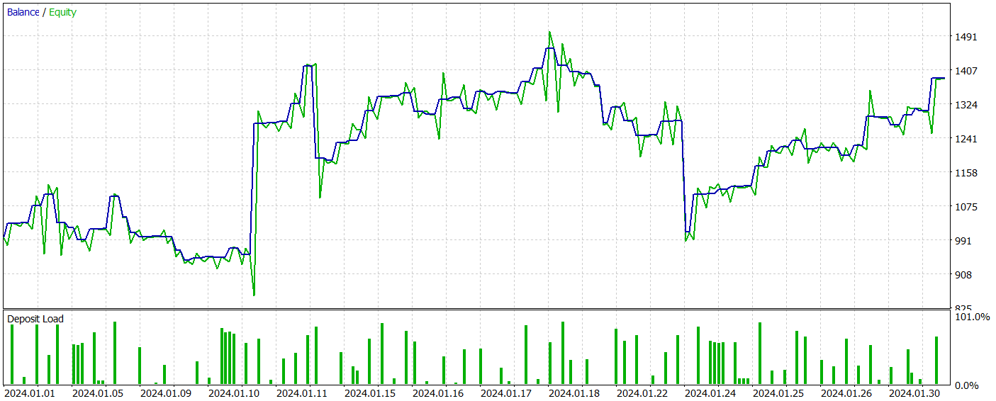
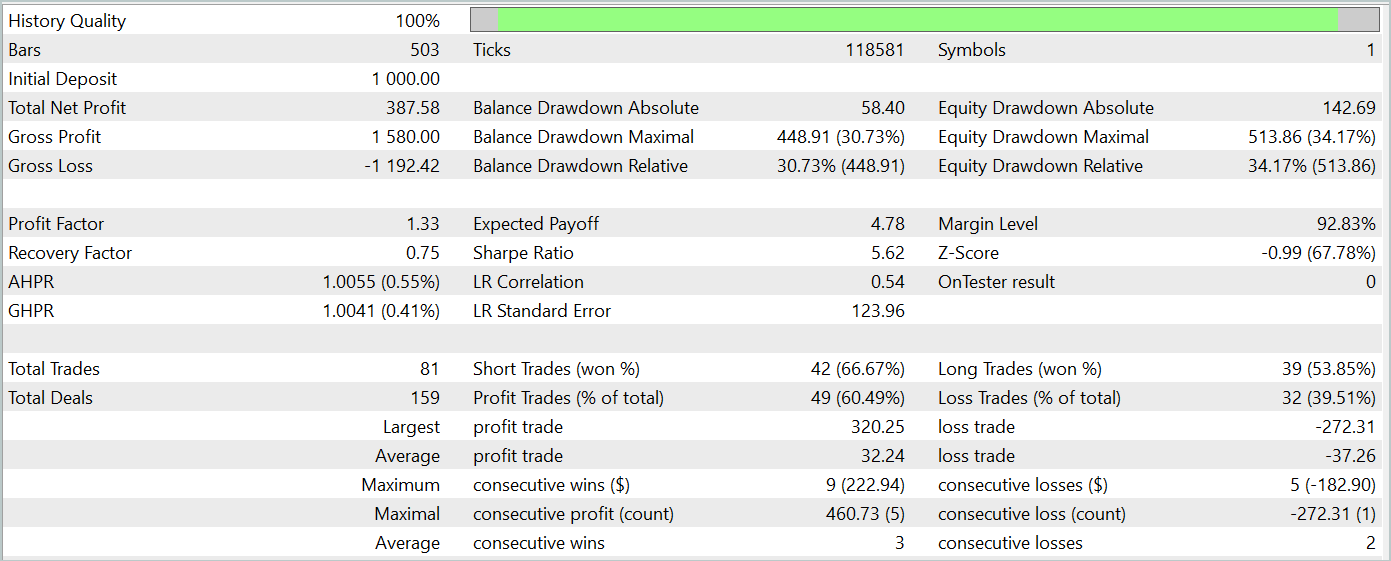
During the testing period, the model executed 81 trades. The distribution between short and long positions was almost equal: 42 versus 39, respectively. More than 60% of the trades were closed with a profit, leading to a profit factor of 1.33.
One distinctive feature of the SparseTSF method is forecasting data in terms of individual steps within the cyclicity period of the original data. As a reminder, in the trained environmental state Encoder model, we analyzed hourly data with a 24-hour cyclicity period. This aspect makes the model's profitability particularly interesting when viewed on an hourly basis.
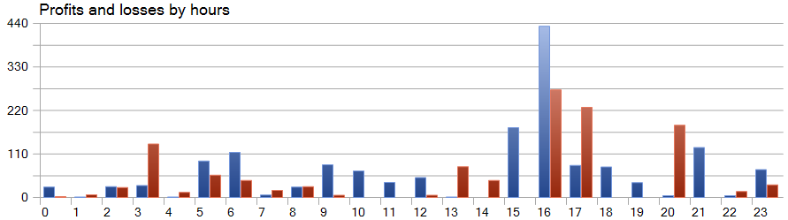
In the presented graph, we observe a near absence of losses during the first half of the European session, from 9:00 to 12:00. The average duration of a trade being 1 hour and 6 minutes indicates minimal delay between entering the trade and realizing profit/loss. The highest profitability occurs at the start of the American session (15:00 - 16:00).
Conclusion
In this article, we introduced the SparseTSF method, which demonstrates advantages in time series forecasting due to its lightweight architecture and efficient resource usage. The minimal number of parameters makes the proposed model especially useful for applications with limited computational resources and a short decision-making time.
SparseTSF allows for the analysis of individual steps in time series with a given periodicity, making independent forecasts for each unitary sequence. This provides the model with high flexibility and adaptability.
In the practical part of the article, we implemented the proposed approaches using MQL5, trained the model, and tested it on real historical data. As a result, we obtained a model capable of generating profits on both training and test datasets, indicating the effectiveness of the proposed approaches.
However, I want to remind you once again that the programs presented in this article are intended only to demonstrate one variant of the implementation of the proposed approaches and their use. The presented programs are not ready for use in real financial markets.
References
Programs used in the article
| # | Name | Type | Description |
|---|---|---|---|
| 1 | Research.mq5 | Expert Advisor | Example collection EA |
| 2 | ResearchRealORL.mq5 | Expert Advisor | EA for collecting examples using the Real-ORL method |
| 3 | Study.mq5 | Expert Advisor | Model training EA |
| 4 | StudyEncoder.mq5 | Expert Advisor | Encoder training EA |
| 5 | Test.mq5 | Expert Advisor | Model testing EA |
| 6 | Trajectory.mqh | Class library | System state description structure |
| 7 | NeuroNet.mqh | Class library | A library of classes for creating a neural network |
| 8 | NeuroNet.cl | Code Base | OpenCL program code library |
Translated from Russian by MetaQuotes Ltd.
Original article: https://www.mql5.com/ru/articles/15392
Warning: All rights to these materials are reserved by MetaQuotes Ltd. Copying or reprinting of these materials in whole or in part is prohibited.
This article was written by a user of the site and reflects their personal views. MetaQuotes Ltd is not responsible for the accuracy of the information presented, nor for any consequences resulting from the use of the solutions, strategies or recommendations described.

 Mastering Log Records (Part 5): Optimizing the Handler with Cache and Rotation
- Free trading apps
- Over 8,000 signals for copying
- Economic news for exploring financial markets
You agree to website policy and terms of use