Neural Network in Practice: Pseudoinverse (II)

Introduction

I am glad to welcome everyone to a new article about neural networks. 

In the previous article "Neural Network in Practice: Pseudoinverse (I)", I showed how you can use a function available in the MQL5 library to calculate the pseudoinverse. However, the method present in the MQL5 library, as in many other programming languages, is intended to calculate the pseudoinverse when using matrices or at least some structure that may resemble a matrix.

Although this article shows how to perform multiplication of two matrices, and even factorization to get the determinant of any matrix (which is important to know whether a matrix can be inverted or not), we still have to implement one more factorization. This is necessary so that you can understand how factorization is performed to obtain pseudoinverse values. This factorization consists of generating the inverse matrix.

But what about transposition? Well, in the previous article, I showed how to perform a factorization that simulates the multiplication of a matrix by its transpose. So, executing such an operation is not an issue.

However, the calculation we have yet to implement, i.e. finding the inverse of a matrix, is not something I intend to cover in detail. Not due to complexity but because these articles are intended to be educational rather than instructional for implementing specific functionalities. Therefore, I decided to take a different approach in this article. Instead of focusing on the generic factorization required to compute the inverse of a matrix, we will delve into the factorization of the pseudo-inverse using the data we've been working with from the beginning. In other words, rather than presenting a generic method, we'll take a specialized approach. The best part is that you will understand much better why everything works the way it does than if we followed the general logic in creating the factorization, as shown in the previous article, where these functions were general. You will see that computations can be performed much faster if we do it in a specialized way. Now, let's explore a new topic to better understand this concept.

Why Generalize When We Can Specialize?

The title of this section may seem controversial, or at least difficult to understand for some. Many programmers prefer to develop highly generic solutions. They believe that by creating generic implementations, they will have tools that are broadly applicable and often efficient. They strive to design solutions that will work in any scenario. However, this pursuit of generalization can come at costs that are not always necessary. If a specialized approach achieves the same goal more effectively, why generalize? In such cases, generalization offers no meaningful advantages.

If you think that I am saying strange things, let's discuss this a little, and then you will understand what I want to explain. Let me guide you through an example to illustrate the point. Consider the following questions:

What is a computer, and why does it contain so many components? Why do new hardware innovations frequently replace software solutions?

If you're under 40 years old or born after 1990 and haven't studied older technologies, what I'm about to say might seem surprising. In the 1970s and early 1980s, computers were nothing like they are today. To give you an idea, video games were entirely programmed in hardware using transistors, resistors, capacitors, and other discrete components. Software-based games did not exist. Everything was implemented in hardware. Now, imagine the difficulty of creating even a simple game like PONG with just electronic components. The engineers of the time were incredibly skilled.

However, the use of discrete components, such as transistors, resistors, and capacitors, meant that systems were slow and had to remain simple. When the first assembly kits, like the Z80 or 6502 processors, were introduced, everything began to change. These processors (still available today) made it far easier and faster to program calculations in software than to implement them in hardware. This marked the dawn of the software era. What does this have to do with neural networks and our current implementation? Patience, dear reader, we'll get there.

The ability to program relatively complex tasks using simple instructions made computers extremely versatile. Many innovations begin as software because software is faster to develop and refine. Once refined, certain features may then transition to hardware implementations for greater efficiency. This progression is evident in GPUs , where many features initially developed in software are optimized over time before being incorporated into hardware. This brings us back to the point of this discussion. While generalization is possible, it often introduces inefficiencies - not during development, but in execution. Generic implementations frequently require additional testing to ensure no unexpected errors occur during execution. On the other hand, specialized approaches are less error-prone and can be optimized for faster execution.

You might wonder why this matters when working with just four values in a database. Here is the reason, dear reader. We often start creating a system able to work with a small dataset, gradually scaling to handle larger volumes of data. Eventually, execution times become inefficient. That's when hardware specialization becomes necessary to perform the same computations that were previously performed using software. This is precisely how new hardware technologies are born.

If you've been following hardware development, you've likely noticed a trend toward specialized technologies. But why is that? This trend occurs because software-based solutions eventually become less cost-effective than hardware-based alternatives. Before rushing to purchase a new GPU advertised as accelerating neural network computations, it's important to first understand how to optimize the hardware you already have. This requires specialized calculations instead of generic ones. For this reason, we'll focus on optimizing calculations for the pseudoinverse. So, instead of creating an article with generic computations showing how to factorize a pseudoinverse, I decided to implement a more specialized calculation. Although please note that it will not be optimized in terms of computing power, since its purpose is training, which is not efficient in this regard. By optimizing I mean the way everything will be implemented. We are not going to reach a the maximization of computing power where it becomes necessary to implement factorization on specialized hardware. This is exactly what happens when new equipment technology emerges.

There has been a lot of talk about GPUs and CPUs with neural network computing capabilities. But is this approach really what you need? To answer this question, we first need to understand what is going on from a software perspective. Let's now move on to the next topic where we will see what will be implemented in terms of software.

Pseudoinverse: A Proposed Approach

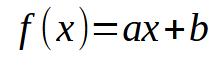
By now, I hope you understand the key points. Let's now consider the following: In our database, each piece of information can be visualized as a two-dimensional plot with X and Y coordinates. This visualization allows us to establish mathematical relationships between data points. From the beginning of this series, we've explored linear regression as a means to achieve this. In previous articles, I explained how to perform a scalar calculation to find the slope and intercept, which allowed us to derive the equation shown below.

In this case, the desired points are the values < a > and < b >. However, there's another approach involving matrix factorization. Specifically, we need to implement a pseudoinverse. The calculations for this are given below.

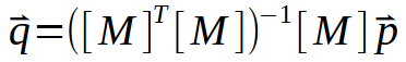
Here the values of the constants < a > and < b > are in the vector < q >. To compute < q >, matrix M must undergo a series of factorizations. However, the most interesting part lies in the process shown in the following figure:

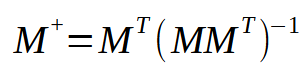
This image is exactly what we need to implement. It represents what happens in the pseudoinverse. Note that the resulting matrix has a special name: pseudoinverse. As you can see in the figure above, it is multiplied by vector < p >, resulting in vector < q >. This vector < q > is the result we want to obtain.

In the previous article and at the beginning of this article we mentioned that the pseudoinverse function is implemented in libraries, so matrices are used for it. But here we do not use matrices, we use something similar to them: arrays. So, at this point we have a problem whose solution is either convert the array to a matrix or implement a pseudoinverse for the arrays. Since I want to show how the computation is implemented, we will choose the second approach, that is, the pseudoinverse implementation. The relevant calculations are shown below.

01. //+------------------------------------------------------------------+
02. matrix __PInv(const double &A[])
03. {
04.     double M[], T[4], Det;
05. 
06.     ArrayResize(M, A.Size() * 2);
07.     M[0] = M[1] = 0;
08.     M[3] = (double)A.Size();
09.     for (uint c = 0; c < M[3]; c++)
10.     {
11.         M[0] += (A[c] * A[c]);
12.         M[2] = (M[1] += A[c]);
13.     }
14.     Det = (M[0] * M[3]) - (M[1] * M[2]);
15.     T[0] = M[3] / Det;
16.     T[1] = T[2] = -(M[1] / Det);
17.     T[3] = M[0] / Det;
18.     ZeroMemory(M);
19.     for (uint c = 0; c < A.Size(); c++)
20.     {
21.         M[(c * 2) + 0] = (A[c] * T[0]) + T[1];
22.         M[(c * 2) + 1] = (A[c] * T[2]) + T[3];
23.     }
24. 
25.     matrix Ret;
26.     Ret.Init(A.Size(), 2);
27.     for (uint c = 0; c < A.Size(); c++)
28.     {
29.         Ret[c][0] = M[(c * 2) + 0];
30.         Ret[c][1] = M[(c * 2) + 1];
31.     }
32. 
33.     return Ret;
34. }
35. //+------------------------------------------------------------------+

This fragment, presented above, does all the work for us. It may appear somewhat complicated at first glance, but in reality, it is quite straightforward and efficient. Essentially, we are dealing with an array that holds various 'double' values. While we could use other types, it is important that you, my dear reader, begin to familiarize yourself with using 'double' values from this point onward. The reason for this will become clear soon. Once all the factorization steps are completed, we will receive a matrix of double values as the result.

Now, pay attention: The array we are working with is a simple one. However, we will treat it as if it were a matrix with two columns. But how is this possible? Let's understand into this before discussing how we can use this code.

In line 6, we create a matrix that will have as many rows as there are elements in the array. But it will have two columns. This differs from the array, which only has a single column internally. In lines 7 and 8, we initialize the matrix M in a very specific manner. To understand this, take a look at the image below.

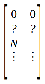
Observe that the first two positions are set to zero, followed by two other positions marked with question marks, as we don't yet know their exact values. Shortly after, we have a position marked with N. This value N represents the size of the array. But why are we placing the size of the array in the matrix? The reason is simple: it is faster to access a value at a known position than to look for the same value using a function. Since we need four free positions at the beginning of the matrix, we place the size of the array in the position labeled N. This is what is being done in lines 7 and 8.

Now, as shown in the previous image, the first step we need to perform is the multiplication of a matrix by its transpose. But here, we don't have a matrix. All we have is an array, or more accurately, a vector. So how do we perform the multiplication? It's quite simple. We use the loop on line 9 to accomplish this. But what is this loop doing? It might seem puzzling at first glance, but let's break it down by looking at the following image.

An array is essentially a collection of values, represented here from a0 to an. If you think about it, rather than viewing it as an array, you can think of it as either a matrix with a single column or a matrix with a single row, depending on how the data is organized. Now, when you perform an operation between a matrix with one column and another matrix with one row, you get a scalar value rather than a matrix. Remember that the formula for the pseudoinverse first requires the multiplication of a matrix by its transpose. However, we can implicitly consider the array shown above as a matrix. See the image below.

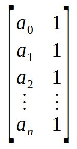
Wow! Now, we have the matrix that we need. By multiplying an n x 2 matrix by its transpose, we end up with a 2 x 2 matrix. In other words, we have successfully transformed an array, or more accurately, a vector, into a 2 x 2 matrix. This is exactly what the for loop in line 9 is doing - multiplying a matrix by its transpose and placing the result at the top of the matrix declared on line 6.

Next, we need to find the inverse of the matrix we just constructed. For a 2 x 2 matrix, the fastest and simplest way to calculate the inverse is using the determinant. Here's the important fact: we don't need a generic method to find the inverse matrix or the determinant. We also don't need a generic way to multiply the matrix by its transpose. We can handle all of this directly, as we've reduced everything to a simple 2 x 2 matrix, making the task much simpler and faster. So, to calculate the determinant, we use line 14. Now, we can go ahead and compute the inverse of the matrix. This inverse calculation, which would be slow if implemented generically, is completed extremely quickly due to the choices we've made. From lines 15 to 17, we generate the inverse in the matrix obtained via the array. At this point, almost everything is ready. The next step is to clear the matrix M, which is done in line 18. Now, pay attention. Matrix T contains the inverse matrix, and array A contains the values we want to factorize into the pseudoinverse. All that remains is to multiply one by the other and place the result into matrix M. The key detail here is that matrix T is 2 x 2, while the array A can be viewed as an n x 2 matrix. This multiplication will result in an n x 2 matrix that contains the values of the pseudoinverse.

This factorization is performed in the loop in line 19. In lines 21 and 22, we place the values into matrix M. And voilà, we have the result of the pseudoinverse. The process I'm describing here could be ported into an OpenCL block, using the GPU capabilities to compute linear regression for a very large database. In some cases, using the CPU would result in calculations taking several minutes, but sending the task to the GPU would make it much faster. This is the optimization I mentioned earlier in this article.

Now we only need to place the result from array M into a matrix. This is done in lines 25 to 31. What you find within M already represents the desired result. In the attachment, I'll provide the code so you can see how everything works and compare it with what was shown in the previous article. However, not everything is perfect. Note that I'm not performing any tests within this function. This is because, although the function is educational, the goal here is to make it resemble something that could be implemented in hardware. In that case, tests would be performed differently, saving us processing time.

Now, this doesn't answer a crucial question: How can this PInv (pseudoinverse) function generate linear regression results so quickly? To answer this, let's move on to the next topic.

Maximum Speed

In the previous section, we saw how, based on an array, we could perform the calculation of the pseudoinverse. However, we can accelerate this process even further. Instead of returning just the pseudoinverse, we can return the linear regression values. To do this, we will need to make some slight adjustments to the code from the previous section. These changes will be enough to allow us to use the full speed of the GPU or a dedicated CPU to find the factors of the linear equation. The sought coefficients are the slope and the point of intersection. The updated fragment can be seen below.

01. //+------------------------------------------------------------------+
02. void Straight_Function(const double &Infos[], double &Ret[])
03. {
04.     double M[], T[4], Det;
05.     uint n = (uint)(Infos.Size() / 2);
06. 
07.     if (!ArrayIsDynamic(Ret))
08.     {
09.         Print("Response array must be of the dynamic type...");
10.         Det = (1 / MathAbs(0));
11.     }
12.     ArrayResize(M, Infos.Size());
13.     M[0] = M[1] = 0;
14.     M[3] = (double)(n);
15.     for (uint c = 0; c < n; c++)
16.     {
17.         M[0] += (Infos[c * 2] * Infos[c * 2]);
18.         M[2] = (M[1] += Infos[c * 2]);
19.     }
20.     Det = (M[0] * M[3]) - (M[1] * M[2]);
21.     T[0] = M[3] / Det;
22.     T[1] = T[2] = -(M[1] / Det);
23.     T[3] = M[0] / Det;
24.     ZeroMemory(M);
25.     for (uint c = 0; c < n; c++)
26.     {
27.         M[(c * 2) + 0] = (Infos[c * 2] * T[0]) + T[1];
28.         M[(c * 2) + 1] = (Infos[c * 2] * T[2]) + T[3];
29.     }
30.     ArrayResize(Ret, 2);
31.     ZeroMemory(Ret);
32.     for (uint c = 0; c < n; c++)
33.     {
34.         Ret[0] += (Infos[(c * 2) + 1] * M[(c * 2) + 0]);
35.         Ret[1] += (Infos[(c * 2) + 1] * M[(c * 2) + 1]);
36.     }
37. }
38. //+------------------------------------------------------------------+

Note that in the code above the check is already running. This check verifies whether the returned array is of dynamic type. Otherwise, the application will need to be closed. The closing occurs in line 10. In the previous article, I explained the significance of this line (refer to it for further details if necessary). Other than that, most of the code continues to function in much the same way as discussed in the previous section, up until line 30, where things take a different direction. But let's step back for a moment. Looking at this code, you might find it unusual, particularly the way the transpose is multiplied with the matrix, or rather, the array, and how the inverse matrix is then multiplied with the original matrix to compute the pseudoinverse.

What is the meaning of what we see in this fragment? What appears to be something very complex is nothing more than a "matrix of points". To better understand, refer to the image below.

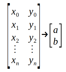
Notice that we have one "matrix" entering and another "matrix" exiting. In the declaration on line 2, the parameter Infos represents the first matrix shown in the image, while Ret represents the second matrix. The values < a > and < b > are the coefficients we are trying to determine to construct the equation of the line. Now, pay close attention: Rach row of the matrix on the left represents a point on the graph. The even-indexed values correspond to those used in the function discussed earlier. Meanwhile, the odd-indexed values represent the vectors in the formula mentioned at the beginning of this article. i.e , the vector < p >.

This function, discussed at the beginning of this topic, takes all the points on the graph and returns the linear regression equation. To achieve this, we must separate the data in some way, and the way to do this is by organizing the even and odd values. This is why the code appears so different from the one in the previous section. However, they function in the same way, at least until line 30. At that point, we perform something not seen in the earlier code. Here, we take the result of the pseudoinverse stored in the matrix M and multiply it by the vectors found in the odd-indexed positions of the Infos parameter. This produces the Ret vector, which consists of the constants needed to define the equation of the line, or linear regression, as you prefer.

If you perform the same operation using the values returned by the PInv function from the previous article, you will arrive at the same result as the one shown in this fragment. The only difference is that this particular implementation is designed to be suitable for hardware-based execution, such as in a dedicated neural network computation unit. This can lead to new technologies being integrated in processors, allowing manufacturers to claim that a given processor or circuit has built-in artificial intelligence or neural network capabilities. However, this is not revolutionary or groundbreaking. It simply involves implementing in hardware something that was previously executed in software, converting a generic system into a specialized one.

Final considerations

My dear readers and enthusiasts. With everything discussed thus far, I believe we have covered all you need to know about neural networks and artificial intelligence at this stage. However, so far we have not discussed the neural network as such, but the use and construction of a single neuron, since we have only performed one calculation. In a neural network, the same calculations are performed multiple times, but on a larger scale. Even if this isn't immediately apparent to you, a neural network is simply the implementation of a graph architecture, where each node represents a neuron or a linear regression function. Depending on the computed results, certain pathways are followed.

I understand that this perspective might seem uninspiring, even trivial. But this is the reality. There is nothing magical or fantastical about neural networks, no matter how the media or uninformed individuals portray them. Everything done by a machine is nothing more than simple mathematical calculations. If you understand these calculations, you will understand neural networks. Moreover, you will gain insights into how to simulate the behavior of living organisms. It is not because living organisms are organic machines, though in some cases, we could argue they are. But that's a conversation for another time.

What I hope for you, my esteemed reader, is that you grasp the essence of a neural network at its simplest level by understanding the concept of a single neuron, which is precisely what we have explored so far.

In upcoming articles, I will guide you through organizing a single neuron into a small network, enabling it to learn something. I deliberately avoid applying these concepts to financial markets, so don't expect to see that from me in the future. My goal is to help you understand, learn, and be able to explain through your own experience what a neural network is and how it learns. To do this, you will need to experiment with a system that is simple enough to grasp.

So, stay tuned for a continuation of this topic. I will think of something exciting to share with you, something truly worth exploring. Meanwhile, the attached materials contain the necessary code for you to start studying how a single neuron works.