Neural Network in Practice: Pseudoinverse (I)

Introduction

I am glad to welcome everyone to a new article about neural networks.

In the previous article "Neural network in practice: Straight Line Function", we were talking about how algebraic equations can be used to determine part of the information we are looking for. This is necessary in order to formulate an equation, which in our particular case is the equation of a straight line, since our small set of data can actually be expressed as a straight line. All the material related to explaining how neural networks work is not easy to present without understanding the level of knowledge of mathematics of each reader.

While many may think that this process would be much simpler and more straightforward, especially considering that there are many libraries on the Internet promising that you can develop your own neural network, the reality is that it is not that simple.

I don't want to give false expectations: I'm not going to tell you that with virtually no knowledge or experience you can create something really practical that can be used to make money using Neural Networks or Artificial Intelligence to trade the market. If someone tells you this, then they are definitely lying.

Creating even the simplest neural network is a challenging task in many cases. Here I want to show you how you can create something that will inspire you to explore this topic in more depth. Neural networks have been the subject of research for at least several decades. As mentioned in the three previous articles on artificial intelligence, the topic is much more complex than many people think it to be.

Using a particular function does not mean that our neural network will be better or worse, it just means that we will perform calculations using a particular function. This relates to what we will see in this article today.

Compared to the first three articles in the series on neural networks, after today's article you may think about giving up. You shouldn't. Because the very same article can also push you to delve deeper into the topic. Here we will look at how pseudo-inverse calculations can be implemented using pure MQL5. While it doesn't look that scary, today's code will be much more difficult for beginners than we would like it to be, so don't be scared. Study the code carefully and calmly, without rushing. I, in turn, tried to make the code as simple as possible. As such, it is not designed to be executed efficiently and quickly. On the contrary, it strives to be as educational as possible. However, since we will be using matrix factorization, the code itself is a bit more complex than what many are used to seeing or programming.

And yes, before anyone mentions it, I know that MQL5 has a function called PInv that does exactly what we'll see in this article. I also know that MQL5 has functions for matrix operations. But here we will not perform calculations using matrices as defined in MQL5, here we will use arrays, which although similar, have a slightly different logic for accessing elements located in memory.

Pseudoinverse

Implementing this calculation is not one of the most difficult tasks, as long as everything is clear to the developer. Basically, we need to perform some multiplications and other simple operations using just one matrix. The output will be a matrix that is the result of all internal factorizations of the pseudoinverse.

At this stage we need to clarify something. The pseudoinverse can be factorized in two ways: in one case, the values inside the matrix are not ignored, and in the other, the minimum limit value is used for the elements present in the matrix. If this minimum limit is not reached, the value of this element in the matrix will be zero. This condition is not imposed by me, but by the rules embedded in the calculation model used by all programs that calculate the pseudoinverse. Each of these cases has a very specific purpose. So what we see here is NOT the final calculation for the pseudoinverse. We will perform a calculation whose purpose is to obtain results similar to those obtained by programs such as MatLab, SciLab and others that also implement the pseudoinverse.

Since MQL5 can also calculate pseudoinverse, we can compare the results obtained using the application we implement with the same results obtained using the MQL5 library pseudoinverse function. This is necessary in order to check if everything is correct. Thus, the goal of this article is not just to implement pseudoinverse calculations, but to understand what is behind it. This is important because knowing how computation works will allow you to understand why and when to use a particular method in our neural network.

Let's start with implementing the simplest code for using pseudoinverse from the MQL5 library. This is the first step to make sure that the calculation we will create later actually works. Please do not change the code without checking it first. If you change anything before this, you may get different results than those shown here. So first try the code I'm going to show you. Then, and only then (if you wish), change it to better understand what's going on, but please don't make any changes to the code before testing the original version.

The original codes are available in the attachment to this article. Let's look at the first one. The full code is shown below:

01. //+------------------------------------------------------------------+
02. #property copyright "Daniel Jose"
03. //+------------------------------------------------------------------+
04. void OnStart()
05. {
06.     matrix M_A {{1, -100}, {1, -80}, {1, 30}, {1, 100}};
07. 
08.     Print("Moore–Penrose inverse of :");
09.     Print(M_A);
10.     Print("is :");
11.     Print(M_A.PInv());
12. }
13. //+------------------------------------------------------------------+

The result of the code execution is shown in the image below:

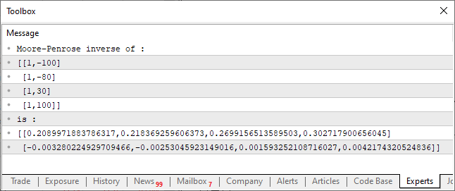
This very simple code that you can see above is able to calculate the pseudoinverse of a matrix. The result is displayed on the console as shown in the figure. Everything is quite simple. However, pay attention to the construction of the code, this is a very specific point in terms of code creation. Using a matrix and a vector, we obtain a whole range of possible and quite functional operations. These operations are included in the standard MQL5 library and can also be included in the standard libraries of other languages.

While this is very useful, there are times when we need or want the code to execute in a specific way. Either because we want to optimize it somehow, or simply because we don't want to generate code that can be executed in another way. In the end, the reason doesn't matter that much. Although many people say that C/C++ programmers like to reinvent the wheel, this is not the case with us. In this article, we'll take a look together at what's behind those complex calculations. You see the result but have absolutely no idea how it was achieved. Any research without understanding where exactly this result came from, and not some other, is not real research, it is just faith. In other words, you see it and you just believe it, but you don't know if it's true or not, you just have to believe it. And real programmers can't blindly trust, they need to touch, see, taste and experience to truly believe in what they are creating. Let's now see how the result shown in the figure was achieved. To do this, let's move on to a new topic.

Understanding the computations behind the pseudoinverse

If you are happy with just seeing results without knowing how they were achieved, that is great. This means that this topic will no longer be useful to you, and you should not waste your time reading it. But if you want to understand how the computations are done, be prepared. Although I will try to simplify the process as much as possible, you will still have to be attentive. I will avoid using complex formulas as much as possible, but your attention is still important here, as the code we will be creating may look much more complicated than it actually is. Let's start with the following: The pseudoinverse is basically calculated using matrix multiplication and inverse.

This multiplication is quite simple. Many people use some resources for this purpose that I personally find unnecessary. In the articles where we talked about matrices, we discussed a method for performing multiplication, but that method was intended for a rather specific scenario. Here we need a slightly more general method because we will have to do a few things different from what we saw in the article on matrices.

To make things easier, we'll look at the code in small parts, each explaining something specific. Let's start with multiplication, which can be seen below:

01. //+------------------------------------------------------------------+
02. void Generic_Matrix_A_x_B(const double &A[], const uint A_Row, const double &B[], const uint B_Line, double &R[], uint &R_Row)
03. {
04.     uint A_Line = (uint)(A.Size() / A_Row),
05.          B_Row  = (uint)(B.Size() / B_Line);
06. 
07.     if (A_Row != B_Line)
08.     {
09.         Print("Operation cannot be performed because the number of rows is different from that of columns...");
10.         B_Row = (uint)(1 / MathAbs(0));
11.     }
12.     if (!ArrayIsDynamic(R))
13.     {
14.         Print("Response array must be of the dynamic type...");
15.         B_Row = (uint)(1 / MathAbs(0));
16.     }
17.     ArrayResize(R, A_Line * (R_Row = B_Row));
18.     ZeroMemory(R);
19.     for (uint cp = 0, Ai = 0, Bi = 0; cp < R.Size(); cp++, Bi = ((++Bi) == B_Row ? 0 : Bi), Ai += (Bi == 0 ? A_Row : 0))
20.         for (uint c = 0; c < A_Row; c++)
21.             R[cp] += (A[Ai + c] * B[Bi + (c * B_Row)]);
22. }
23. //+------------------------------------------------------------------+

Looking at this piece of code, you might already feel disoriented. Someone might be terrified as if end of the world is approaching. Others might want to ask God for forgiveness for all their sins. But jokes aside, this code is very simple, even if it seems unusual or extremely complex.

You may find it difficult because it is very compressed and seems to have many things happening at once. I apologize to the beginners, but those of you who have been following my articles already know my style of writing code, and you will see that this is my typical style. Let's now figure out what's going on here. Unlike the code shown earlier, this code is general, it even has a test that checks if we can multiply two matrices. This is quite useful, although not very convenient for us.

In the second line we have the procedure declaration. We must be careful to declare and pass parameters in the right places. Then matrix A will be multiplied by matrix B and the result will be placed into matrix R. We need to specify how many columns matrix A has and how many rows matrix B has. The last argument will return the number of columns in matrix R. The reason for returning the number of columns in the R matrix will be explained later, so don't worry about it for now.

Fine. In the fourth and fifth lines we will calculate the remaining values so that we don't have to specify them manually. Then, in line 7, we do a little test to see if matrices can be multiplied, so the order in which matrices are passed matters. This is what differs it from the code for scalar computations: in matrix computations we have to be very careful.

If the multiplication fails, then in the ninth line we will output a message to the MetaTrader 5 console. And right after that, in line ten, a RUN-TIME error will be thrown, which will cause the application that is trying to perform matrix multiplication to close. If such an error appears on the console, you will need to check whether the message also appears in the ninth line. If this happens, the error will not be in the code fragment in question, but at the point where this code is called. I know that forcing the application to close on RUN-TIME error is not very nice, let alone elegant, but this way we will prevent the application from showing us incorrect results.

Now comes the part that starts to scare a lot of people: in line 17, we allocate memory to store the entire output. Thus, the matrix R must have a dynamic form in the caller. Don't use a static array because then line 12 will detect this and the code will exit with a RUN-TIME error with a message in line 14 indicating the reason for exiting.

One of the details of this error generation method is that when executed, the application will attempt to divide by zero, which will cause the processor to trigger an internal interrupt. This interrupt will cause the operating system to take action against the application that caused the interrupt and force it to close. Even if the operating system does nothing, the processor will go into interrupt mode, causing it to terminate, even in an embedded system designed to run an application.

Now, the thing to notice is that here I use a trick to prevent the compiler from detecting that a RUN-TIME error will be generated. If I did it differently than shown in the code, the compiler would fail to compile the code, even though the line causing the RUN-TIME error would rarely be executed in normal situations. If you need to forcefully terminate a program, you can use a similar technique, it always works. Although this is not very elegant, because the user may be angry with your application or with you who wrote it. So use this approach wisely.

In line 18 we completely clear everything that is in the allocated memory. Usually some compilers do the cleanup themselves, but after some time of programming in MQL5 I noticed that it naturally does not clean up dynamically allocated memory. I believe this is because dynamically allocated memory in MetaTrader 5 is intended for use in indicator buffers. And since these buffers are updated as data is received and calculated, there is no point in clearing the memory. In addition, such cleaning takes a lot of time, which can be spent on other tasks. So we must do this cleaning and make sure we're not using unnecessary values in our calculations. Please pay attention to this in your programs if you use dynamically allocated memory and it is not used as user indicator buffers.

Continuing, now comes the most interesting part of the procedure: we multiply matrix A by matrix B and place the result in matrix R. This is done in two lines. Line 19 may seem very complicated at first glance, but let's break it down into pieces. The idea is to make the multiplication of two matrices completely dynamic and universal. That is, it does not matter whether there are more or fewer rows or columns, if the procedure has reached this point, the matrices will be multiplied.

Just as the order of the matrices affects the result, here in line 19 the order in which the operations are performed also affects the result. To avoid going on too long, I will simplify the explanation. To understand what's going on, let's read the code as it's written, that is, from left to right, term by term. This is how the compiler processes it to create the executable, so while it may seem confusing, it isn't. The code is very concise and different from what most people use. In any case, the idea is to read column by column from matrix A and multiply the value by reading row by row from matrix B. For this reason, the order of the coefficients will affect the result. You don't need to worry about how matrix B is organized (row or column), it can be organized the same way as matrix A and this multiplication procedure will still succeed.

The first of the operations needed to obtain the value of the pseudoinverse is ready. Now let's look at the kind of computations we need to perform so we know what else we need to implement. We may not need a general solution like in the case of multiplication, but something more specific to help determine the value of the pseudoinverse.

The formula for calculating the pseudoinverse is given below.

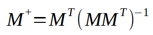
In this formula, M represents the matrix used. Note that it is always the same. However, when looking at this formula, we notice that we need to perform a multiplication between the original matrix and its transposed matrix. Then we take the result and find the value of the inverse matrix. And finally, we multiply the transposed matrix by the result of the inversion. Sounds simple, doesn't it? Here we can create several shortcuts. Of course, to create a perfect shortcut, we would need to model a procedure that can only compute the pseudoinverse. But creating such a procedure, while not difficult, makes it much more difficult to explain how it works. To better understand what I'm talking about, let's do the following: I'll put the multiplication of the transposed and original matrix into one procedure. Usually when we study this issue at university, we are asked to do it in two blocks. That is, we first create the transposed matrix and then use the multiplication procedure to obtain the final result. However, it is possible to create a procedure that does not include these two steps and performs them in one step. While this is very simple to implement, you will find that the code can be difficult to understand.

Let's see in the code below how to perform the operation shown in brackets in the image above.

01. //+------------------------------------------------------------------+
02. void Matrix_A_x_Transposed(const double &A[], const uint A_Row, double &R[], uint &R_Row)
03. {
04.     uint BL = (uint)(A.Size() / A_Row);
05.     if (!ArrayIsDynamic(R))
06.     {
07.         Print("Response array must be of the dynamic type...");
08.         BL = (uint)(1 / MathAbs(0));
09.     }
10.     ArrayResize(R, (uint) MathPow(R_Row = (uint)(A.Size() / A_Row), 2));
11.     ZeroMemory(R);
12.     for (uint cp = 0, Ai = 0, Bi = 0; cp < R.Size(); cp++, Bi = ((++Bi) == BL ? 0 : Bi), Ai += (Bi == 0 ? A_Row : 0))
13.         for (uint c = 0; c < A_Row; c++)
14.             R[cp] += (A[c + Ai] * A[c + (Bi * A_Row)]);
15. }
16. //+------------------------------------------------------------------+

Note that this piece of code is very similar to the previous one, except that the line that produces the result is slightly different in the two pieces. However, this snippet is able to perform the necessary computations to multiply the original matrix by its transposed matrix, saving us from creating the transposed matrix. We can implement this type of optimization. Of course, in this same procedure we could accumulate even more functions, for example, generate an inverse matrix or even perform the multiplication of the inverse matrix by the transposition of the input matrix. But, as you can already imagine, each of these steps complicates the procedure, not globally, but locally. That's why I prefer to introduce it to you little by little so you can understand what's going on and even try out the concepts if you want.

But since I don't want to reinvent the wheel, we won't accumulate everything in one function. I showed this part only to make you understand that not everything we learn in school is applied in practice. Often processes are optimized to solve a specific problem. And optimizing something allows you to get the job done much faster than with a more generalized process.

Next we'll do the following: We already have a multiplication calculation. Next, we need a calculation that generates the inverse of the resulting matrix. There are several ways to program this inverse. Although there are few mathematical ways to express it, programming methods can differ significantly, making one algorithm faster than another. However, what we are really interested in is getting the right result, and how we generate it is not so important.

To compute the inverse of a matrix, I prefer to use a special method that involves using the determinant of the matrix. At this point, you can use another method to find the determinant, but out of habit, I prefer to use the SARRUS method. I think it's easier to program this way. For those who are not familiar with it, I will explain it: Sarrus method computes the determinant based on the values of the diagonals. Programming this is something quite interesting. In the snippet below, you will see one suggestion on how to do this. It works for any matrix, or rather, array, as long as it is square.

01. //+------------------------------------------------------------------+
02. double Determinant(const double &A[])
03. {
04. #define def_Diagonal(a, b)  {                                                                                                                       \
05.                 Tmp = 1;                                                                                                                            \
06.                 for (uint cp = a, cc = (a == 0 ? 0 : cp - 1), ct = 0; (a ? cp > 0 : cp < A_Row); cc = (a ? (--cp) - 1 : ++cp), ct = 0, Tmp = 1)     \
07.                 {                                                                                                                                   \
08.                     do {                                                                                                                            \
09.                         for (; (ct < A_Row); cc += b, ct++)                                                                                         \
10.                             if ((cc / A_Row) != ct) break; else Tmp *= A[cc];                                                                       \
11.                         cc = (a ? cc + A_Row : cc - A_Row);                                                                                         \
12.                     }while (ct < A_Row);                                                                                                            \
13.                     Result +=  (Tmp * (a ? -1 : 1));                                                                                                \
14.                 }                                                                                                                                   \
15.                             }
16. 
17.     uint A_Row, A_Size = A.Size();
18.     double Result, Tmp;
19. 
20.     if (A_Size == 1)
21.         return A[0];
22.     Tmp = MathSqrt(A_Size);
23.     A_Row = (uint)MathFloor(Tmp);
24.     if ((A_Row != (uint)MathCeil(Tmp)) || (!A_Size))
25.     {
26.         Print("The matrix needs to be square");
27.         A_Row = (uint)(1 / MathAbs(0));
28.     }
29.     if (A_Row == 2)
30.         return (A[0] * A[3]) - (A[1] * A[2]);
31.     Result = 0;
32. 
33.     def_Diagonal(0, A_Row + 1);
34.     def_Diagonal(A_Row, A_Row - 1);
35. 
36.     return Result;
37. 
38. #undef def_Diagonal
39. }
40. //+------------------------------------------------------------------+

This beautiful fragment, which can be seen here, manages to establish the value of the determinant of the matrix. Here we are doing something so wonderful that the code doesn't even require any explanation.

In the fourth line, we have a macro defined. This macro is able to traverse an array, or in our case an array within an array, diagonally. That's exactly how it is done. The math behind this code allows you to compute the value of the diagonals one by one, both in the direction of the main diagonal and in the direction of the secondary diagonal, all in an elegant and efficient way. Note that all we need to specify in the code is the array that contains our matrix. The returned value is the determinant of that matrix. However, the Sarrus method, as implemented in this code, has a limitation: if the matrix has 1x1 dimensions, the determinant is the matrix itself, and it is returned immediately, as can be seen in line 21. If the array is empty or not square, we will throw a RUN-TIME error in line 27, preventing the code from executing further. If the matrix size is 2x2, then the calculation of the diagonals does not go through the macro, but is performed before it in line 30. For any other case, the computation of the determinant is done through a macro: First, in line 33, the main diagonal is computed, and in line 34, the secondary diagonal is calculated. If you don't understand what's going on, look at the picture below where I show everything clearly. This is for those who are not familiar with the SARRUS method.

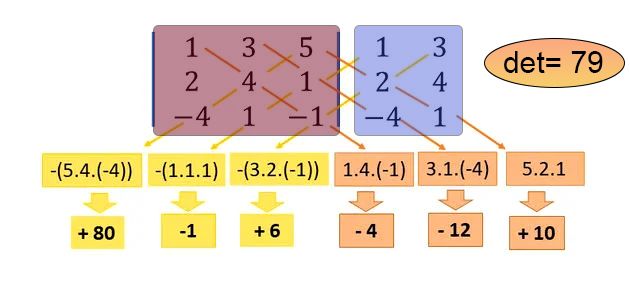
In this image, the area in red represents the matrix for which we want to calculate the determinant, and the area in blue is a virtual copy of some elements of the matrix. The macro code performs exactly the calculation shown in the figure, returning the determinant, which in this example is 79.

Final considerations

Well, dear reader, we have come to the end of another article. However, we have not yet implemented all the necessary procedures for computing the value of the pseudoinverse. We will talk about this in the next article, where we will see an application that will perform this task. While it can be said that we can use the code given in the appendix of this article, the problem is that it does not give us the freedom to use any kind of structure. To use the pseudoinverse (PInv), we actually need to work with a matrix type. In the one I show as an explanation of the calculations, we can use any data modeling. We just need to make the necessary changes to be able to use anything. So, see you in the next article.