
Neural networks made easy (Part 72): Trajectory prediction in noisy environments

Introduction
Predicting the future movement of an asset by analyzing its historical trajectories is important in the context of financial market trading, where analysis of past trends can be a key factor for a successful strategy. Future asset trajectories often contain uncertainty due to changes in underlying factors and the market's reaction to them, which determines many potential future asset movements. Therefore, an effective method for predicting market movements must be able to generate a distribution of potential future trajectories, or at least several plausible scenarios.
Despite the considerable variety of existing architectures for the most likely predictions, models can face the problem of overly simplistic forecasts when predicting the future trajectories of financial assets. The problem persists because the model narrowly interprets the data from the training set. In the absence of clear patterns of asset trajectories, the prediction model ends up generating simple or homogeneous movement scenarios that are unable to capture the diversity of changes in the movement of financial instruments. This can lead to a decrease in forecast accuracy.
The authors of the paper "Enhancing Trajectory Prediction through Self-Supervised Waypoint Noise Prediction" offered a new approach to solving these problems, Self-Supervised Waypoint Noise Prediction (SSWNP), which consists of two modules:
- Spatial consistency module
- Noise prediction module
The first creates two different views of historically observed trajectories: clean and noise-augmented views of the spatial domain of key points. As the name suggests, the clean version represents the original trajectories, while the noise-augmented version represents past trajectories that have been moved in the original feature space with added noise. This approach takes advantage of the fact that the noisy version of past trajectories does not correspond to a narrow interpretation of the data from the training set. The model uses this additional information to overcome the problem of overly simplistic predictions and explore more diverse scenarios. After generating two different past trajectories, we train a future trajectories prediction model to maintain spatial consistency between the predictions from the two and learn spatiotemporal features beyond the movement prediction task.
The noise prediction module solves the auxiliary problem of identifying noise in the analyzed trajectories. This helps the movement prediction model better model potential spatial diversity and improves understanding of the underlying representation in movement prediction, thereby improving future predictions.
The authors of the method conducted additional experiments to empirically demonstrate the critical importance of the spatial consistency and noise prediction modules for SSWNP. When using only the spatial consistency module to solve the movement prediction problem, suboptimal performance of the trained model is observed. Therefore, they integrate both modules in their work.
1. SSWNP Algorithm
The goal of trajectory prediction is to determine the most likely future trajectory of an agent in a dynamic environment based on its previously observed trajectories. A trajectory is represented by a time series of spatial points called waypoints. The observed trajectory covers a period from t1 to tob and can be denoted as
![]()
where Xi* corresponds to coordinates of i at a time step t*. Similarly, the predicted future trajectory for the agent i during the period [tob+1,tfu] can be described as Ŷtob+1≤t≤tfu. Corresponding true trajectory for the future movement of agent i can be described as Ytob+1≤t≤tfu.
In the SSWNP method, two different views of trajectories are first created: one is characterized as a clean view (X≤tob), and the other as a noise-augmented view (Ẍ≤tob). The clean view corresponds to the original trajectory from the training dataset, while the noise-augmented view corresponds to a trajectory that has been moved in the feature space by adding noise.
Noise from the standard normal distribution N(0, 1) is used to distort the clean trajectory. The authors of the method introduce a parameter called noise factor (ω), which controls the spatial movement of waypoints.
![]()
After creating the clean and noise-augmented trajectory views, we feed them to the feature extraction model (Θfe), which generates features corresponding to both the clean view and the noise-augmented view. The resulting features are then fed into a trajectory prediction model (Θsup) to predict trajectories Ŷtob+1≤t≤tfu and Ÿtob+1≤t≤tfu, as shown in the equations below:
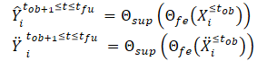
We train the model to minimize the gap between the predicted trajectories and the true trajectory from the training dataset. As can be seen, by minimizing the error in predicting trajectories from clean and noise-augmented initial data (Ŷ and Ÿ) to the true trajectory from the training dataset (Y), we are indirectly reducing the gap between the 2 forecast trajectories. This maintains spatial consistency between future trajectory predictions based on clean observed trajectories and noise-augmented trajectories.

Additionally, the SSWNP method solves the problem of self-supervised noise prediction, which includes predicting the noise present in its clean form, the observed past trajectory X≤tob, as well as in the noise-augmented form Ẍ≤tob. The goal here is to estimate the noise value associated with a given observed waypoint.
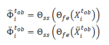
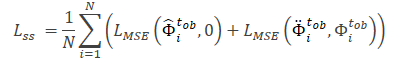
Note that the features extracted by the model Θfe are used as input data for the noise prediction model (Θss), which determines the noise level in the observed trajectories (clean and augmented views). For a loss function for the self-supervised learning of the noise prediction model, the authors of the method propose to use the root mean square error (MSE).
The value 0 here denotes the absence of noise in the clean form trajectory.
The general loss function of the SSWNP method is represented as:
![]()
Where λ denotes the contribution of noise prediction error to the total error when training the model using the proposed approach.
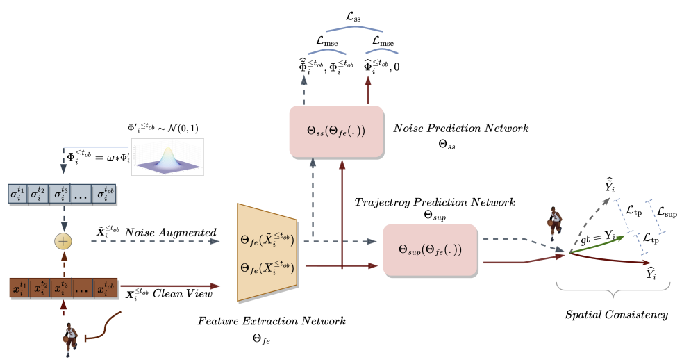
The original visualization of the Self-Supervised Waypoint Noise Prediction method is presented below.
2. Implementation using MQL5
We have seen the theoretical aspects of the Self-Supervised Waypoint Noise Prediction method. As you can see, the proposed approaches do not impose any restrictions on either the architecture of the models used or the structure of the source data. This allows us to integrate the proposed approaches with a large number of algorithms we have previously considered. In particular, in this article we will add the proposed approaches to the autoencoder training algorithm TrajNet, the method we discussed in the recent article on Goal-Conditioned Predictive Coding.
As we discussed previously, the GCPC algorithm provides 2 stages of model training:
The SSWNP method discussed in this article aims to improve the efficiency of predicting future trajectories. Therefore, it covers only the "Trajectory function training" stage. We will make the necessary adjustments to this stage. The second stage, "Behavior policy training" will be used in its existing form.
2.1 Method integration issues
When integrating new approaches into a ready-made structure, we must ensure that the changes we make do not disrupt the already built process. Therefore, before starting our work, we must analyze the impact of new approaches on the previously created learning process and the subsequent operation of the model.
Noise augmentation to the trajectories from the training dataset will obviously change the distribution of the original data. Consequently, this will affect the parameters of the batch normalization layer, in which we pre-process the source data. On the one hand, this is what we are trying to achieve. We want to train a model to work under conditions close to real ones in an environment with high stochasticity. On the other hand, the addition of random noise can push the original data beyond the actual values of the analyzed parameters. To minimize the negative impact of this factor, the authors of the algorithm added a noise factor (ω), which regulates the amount of data shift. In the conditions where we have "raw" non-normalized data, we will need a separate noise factor for each metric of the source data. Thus, we come to using a vector of noise factors. Then selecting a vector of hyperparameters becomes a rather complex task, the complexity of which increases with the increase in the number of analyzed parameters.
The solution to this issue, as it turns out, is quite straightforward. Multiplying noise from a normal distribution by a certain factor is actually quite similar to the reparameterization trick, which we used in the variational autoencoder layer.
![]()
Therefore, by using the parameters of the training dataset distribution, we can keep the model within the original distribution. At the same time, we add the stochasticity inherent in the analyzed environment.
However, one more point must be taken into account here. We add noise to the real trajectories from the training dataset rather than replacing their data with random values. When solving the problem directly, we obtain the distribution parameters of the initial data.
Let's take another look at the idea of using noise. At a specific point in time, we have actual data for each of the analyzed parameters. At the next time step, the parameters change by a certain amount. The size of the change for each parameter depends on a large number of different factors, which brings it close to a random variable. At the same time, such change has its limits. Therefore, in order to preserve the natural distribution of the original data, we can determine the distribution parameters of such deviations between 2 subsequent values of each analyzed parameter. These will be the parameters for reparametrizing our noise.
Here we must take into account the fact that a significant change in parameter values often indicates a change in the market situation. According to the SSWNP method, the model is trained to minimize the gap between trajectory predictions from clean and noisy data. Therefore, we will use the noise factor proposed by the authors of the method to limit the bias from the real trajectories from the training set.
The second point is the use of the DropOut layer in the GCPC method, which also serves as a kind of regularization and is designed to train the model to ignore some "outliers" and restore missing parameters. In the case of combining methods, we have the ignoring of the noise added to the parameters masked by the DropOut layer. On the other hand, parameter masking makes the problem solved by the model much more difficult compared to adding noise.
As mentioned earlier, we should not violate the previously built process. Therefore, we will not exclude the DropOut layer from the Encoder architecture. It will be interesting to observe the model training results.
Now let's look at the construction of the Self-Supervised Waypoint Noise Prediction method. According to algorithm, we will train 3 models:
- feature extraction model
- trajectory prediction model
- noise prediction model
We plan to integrate the SSWNP algorithm into the previously built GCPC process. Let's try to compare the models of both methods. The SSWNP feature extraction model corresponds to the GCPC Encoder. In turn, the GCPC Decoder can be represented as a SSWNP trajectory prediction model. So, we need to add a noise prediction model.
2.2 Model architecture
The model architectures will be described in the CreateTrajNetDescriptions method, to which we will add a description of the third model. In the parameters, the method receives pointers to three dynamic arrays to describe the architecture of these three models. In the body of the method, we check the relevance of the received pointers and, if necessary, create new instances of objects.
bool CreateTrajNetDescriptions(CArrayObj *encoder, CArrayObj *decoder, CArrayObj *noise)
  {
//---
   CLayerDescription *descr;
//---
   if(!encoder)
     {
      encoder = new CArrayObj();
      if(!encoder)
         return false;
     }
   if(!decoder)
     {
      decoder = new CArrayObj();
      if(!decoder)
         return false;
     }
   if(!noise)
     {
      noise = new CArrayObj();
      if(!noise)
         return false;
     }
We copy the description of the Encoder and Decoder architectures without changes. As we have seen in previous articles, we input raw initial data into the Encoder, among which we indicate only historical price changes and analyzed indicators.
//--- Encoder
   encoder.Clear();
//--- Input layer
   if(!(descr = new CLayerDescription()))
      return false;
   descr.type = defNeuronBaseOCL;
   int prev_count = descr.count = (HistoryBars * BarDescr);
   descr.activation = None;
   descr.optimization = ADAM;
   if(!encoder.Add(descr))
     {
      delete descr;
      return false;
     }
They undergo primary processing in the batch normalization layer.
//--- layer 1
   if(!(descr = new CLayerDescription()))
      return false;
   descr.type = defNeuronBatchNormOCL;
   descr.count = prev_count;
   descr.batch = 1000;
   descr.activation = None;
   descr.optimization = ADAM;
   if(!encoder.Add(descr))
     {
      delete descr;
      return false;
     }
The normalized data is randomly masked in the DropOut layer.
//--- layer 2
   if(!(descr = new CLayerDescription()))
      return false;
   descr.type = defNeuronDropoutOCL;
   descr.count = prev_count;
   descr.probability = 0.8f;
   descr.optimization = ADAM;
   if(!encoder.Add(descr))
     {
      delete descr;
      return false;
     }
After that we search for stable patterns using a block of convolutional layers.
//--- layer 3
   if(!(descr = new CLayerDescription()))
      return false;
   descr.type = defNeuronConvOCL;
   prev_count = descr.count = prev_count - 2;
   descr.window = 3;
   descr.step = 1;
   int prev_wout = descr.window_out = 3;
   descr.activation = LReLU;
   descr.optimization = ADAM;
   if(!encoder.Add(descr))
     {
      delete descr;
      return false;
     }
//--- layer 4
   if(!(descr = new CLayerDescription()))
      return false;
   descr.type = defNeuronSoftMaxOCL;
   descr.count = prev_count;
   descr.step = prev_wout;
   descr.optimization = ADAM;
   descr.activation = None;
   if(!encoder.Add(descr))
     {
      delete descr;
      return false;
     }
//--- layer 5
   if(!(descr = new CLayerDescription()))
      return false;
   descr.type = defNeuronConvOCL;
   prev_count = descr.count = prev_count;
   descr.window = prev_wout;
   descr.step = prev_wout;
   prev_wout = descr.window_out = 8;
   descr.activation = LReLU;
   descr.optimization = ADAM;
   if(!encoder.Add(descr))
     {
      delete descr;
      return false;
     }
//--- layer 6
   if(!(descr = new CLayerDescription()))
      return false;
   descr.type = defNeuronSoftMaxOCL;
   descr.count = prev_count;
   descr.step = prev_wout;
   descr.optimization = ADAM;
   descr.activation = None;
   if(!encoder.Add(descr))
     {
      delete descr;
      return false;
     }
Then we process the data in a fully connected layer block.
//--- layer 7
   if(!(descr = new CLayerDescription()))
      return false;
   descr.type = defNeuronBaseOCL;
   descr.count = LatentCount;
   descr.optimization = ADAM;
   descr.activation = LReLU;
   if(!encoder.Add(descr))
     {
      delete descr;
      return false;
     }
//--- layer 8
   if(!(descr = new CLayerDescription()))
      return false;
   descr.type = defNeuronBaseOCL;
   prev_count = descr.count = EmbeddingSize;
   descr.activation = LReLU;
   descr.optimization = ADAM;
   if(!encoder.Add(descr))
     {
      delete descr;
      return false;
     }
We recurrently add the results of previous passes of the Encoder.
//--- layer 9
   if(!(descr = new CLayerDescription()))
      return false;
   descr.type = defNeuronConcatenate;
   descr.count = 2 * EmbeddingSize;
   descr.window = prev_count;
   descr.step = EmbeddingSize;
   descr.optimization = ADAM;
   descr.activation = None;
   if(!encoder.Add(descr))
     {
      delete descr;
      return false;
     }
Then we transfer the data to the internal stack of the history we are analyzing.
//--- layer 10
   if(!(descr = new CLayerDescription()))
      return false;
   descr.type = defNeuronEmbeddingOCL;
   prev_count = descr.count = GPTBars;
     {
      int temp[] = {EmbeddingSize, EmbeddingSize};
      ArrayCopy(descr.windows, temp);
     }
   prev_wout = descr.window_out = EmbeddingSize;
   if(!encoder.Add(descr))
     {
      delete descr;
      return false;
     }
The resulting set of historical data is analyzed in the attention block.
//--- layer 11
   if(!(descr = new CLayerDescription()))
      return false;
   descr.type = defNeuronMLMHAttentionOCL;
   descr.count = prev_count * 2;
   descr.window = prev_wout;
   descr.step = 4;
   descr.window_out = 16;
   descr.layers = 4;
   descr.optimization = ADAM;
   if(!encoder.Add(descr))
     {
      delete descr;
      return false;
     }
The analysis results are compressed by a fully connected layer.
//--- layer 12
   if(!(descr = new CLayerDescription()))
      return false;
   descr.type = defNeuronBaseOCL;
   prev_count = descr.count = EmbeddingSize;
   descr.optimization = ADAM;
   descr.activation = None;
   if(!encoder.Add(descr))
     {
      delete descr;
      return false;
     }
//--- layer 13
   if(!(descr = new CLayerDescription()))
      return false;
   descr.type = defNeuronSoftMaxOCL;
   descr.count = prev_count;
   descr.step = 1;
   descr.optimization = ADAM;
   descr.activation = None;
   if(!encoder.Add(descr))
     {
      delete descr;
      return false;
     }
At the Encoder output, we normalize the data using the SoftMax function.
The results of the Encoder's feed-forward pass are fed into the Decoder.
//--- Decoder
   decoder.Clear();
//--- Input layer
   if(!(descr = new CLayerDescription()))
      return false;
   descr.type = defNeuronBaseOCL;
   descr.count = EmbeddingSize;
   descr.activation = None;
   descr.optimization = ADAM;
   if(!decoder.Add(descr))
     {
      delete descr;
      return false;
     }
In this case, we are dealing with data obtained from the previous model, which has already been normalized. Therefore, there is no need for data pre-processing. We immediately expand them using a fully connected layer.
//--- layer 1
   if(!(descr = new CLayerDescription()))
      return false;
   descr.type = defNeuronBaseOCL;
   prev_count = descr.count = (HistoryBars + PrecoderBars) * EmbeddingSize;
   descr.activation = LReLU;
   descr.optimization = ADAM;
   if(!decoder.Add(descr))
     {
      delete descr;
      return false;
     }
The received data is analyzed in the attention block.
//--- layer 2
   if(!(descr = new CLayerDescription()))
      return false;
   descr.type = defNeuronMLMHAttentionOCL;
   prev_count = descr.count = prev_count / EmbeddingSize;
   prev_wout = descr.window = EmbeddingSize;
   descr.step = 4;
   descr.window_out = 16;
   descr.layers = 2;
   descr.optimization = ADAM;
   if(!decoder.Add(descr))
     {
      delete descr;
      return false;
     }
At the output of the attention block, we have an embedding of each predicted candlestick. To decode the resulting embeddings, we will use a multi-model fully connected layer.
//--- layer 3
   if(!(descr = new CLayerDescription()))
      return false;
   descr.type = defNeuronMultiModels;
   descr.count = 3;
   descr.window = prev_wout;
   descr.step = prev_count;
   descr.activation = None;
   descr.optimization = ADAM;
   if(!decoder.Add(descr))
     {
      delete descr;
      return false;
     }
After describing the architecture of the Encoder and Decoder, we need to add a description of the architecture of the noise prediction model. This model, like the Decoder, uses the results of the Encoder as input data. Therefore, we just copy the original Decoder data layer.
//--- Noise Prediction
   noise.Clear();
//--- Input layer
   if(!(descr = new CLayerDescription()))
      return false;
   descr.Copy(decoder.At(0));
   if(!noise.Add(descr))
     {
      delete descr;
      return false;
     }
Next, using a fully connected layer, we expand the received data to the size of the original data at the Encoder input.
//--- layer 1
   if(!(descr = new CLayerDescription()))
      return false;
   descr.type = defNeuronBaseOCL;
   prev_count = descr.count = HistoryBars * EmbeddingSize;
   descr.activation = LReLU;
   descr.optimization = ADAM;
   if(!noise.Add(descr))
     {
      delete descr;
      return false;
     }
Now attention. At the next step, probably for the first time in the entire series of articles, I created branching for the model architecture depending on the selected hyperparameters. The key here is the number of analyzed candlesticks at the Encoder input. When analyzing more than one candlestick, the model architecture will resemble the Decoder. We use an attention block and a multi-model layer to decode embeddings. Only here we are not talking about forecast candlestick, but about analyzed ones.
//---
   if(HistoryBars > 1)
     {
      //--- layer 2
      if(!(descr = new CLayerDescription()))
         return false;
      descr.type = defNeuronMLMHAttentionOCL;
      prev_count = descr.count = prev_count / EmbeddingSize;
      prev_wout = descr.window = EmbeddingSize;
      descr.step = 4;
      descr.window_out = 16;
      descr.layers = 2;
      descr.optimization = ADAM;
      if(!noise.Add(descr))
        {
         delete descr;
         return false;
        }
      //--- layer 3
      if(!(descr = new CLayerDescription()))
         return false;
      descr.type = defNeuronMultiModels;
      descr.count = BarDescr;
      descr.window = prev_wout;
      descr.step = prev_count;
      descr.activation = None;
      descr.optimization = ADAM;
      if(!noise.Add(descr))
        {
         delete descr;
         return false;
        }
     }
When analyzing only one candlestick at the Encoder input, there is no point of using an attention layer that analyzes the relationships between different candlesticks. Therefore, we will use a simple perceptron.
   else
     {
      //--- layer 2
      if(!(descr = new CLayerDescription()))
         return false;
      descr.type = defNeuronBaseOCL;
      descr.count = LatentCount;
      descr.optimization = ADAM;
      descr.activation = LReLU;
      if(!noise.Add(descr))
        {
         delete descr;
         return false;
        }
      //--- layer 3
      if(!(descr = new CLayerDescription()))
         return false;
      descr.type = defNeuronBaseOCL;
      prev_count = descr.count = BarDescr;
      descr.activation = None;
      descr.optimization = ADAM;
      if(!noise.Add(descr))
        {
         delete descr;
         return false;
        }
     }
//---
   return true;
  }
The above description is only provided for the architectures of the models that participate in the training of the trajectory function model. The architecture of the Agent behavior policy training models is used without changes. You can find them in the attachment. A detailed description was given in the previous article.
2.3 Model training programs
After describing the architecture of the models used, we can move on to consider the algorithms of the programs. Please note that the authors of the SSWNP method do not present requirements for the selection of source data and the collection of observed trajectories for training. Therefore, the programs interacting with the environment are used as is, without any adjustments. The full code of all programs used in the article is available in the attachment and thus you can study them. If clarification is needed, please refer to the previous article or ask a question in the discussion.
We move on to the trajectory function training EA ...\Experts\SSWNP\StudyEncoder.mq5, in which we will simultaneously train 3 models:
- feature extraction model (Encoder)
- trajectory prediction model (Decoder)
- noise prediction model (Noise).
CNet                 Encoder;
CNet                 Decoder;
CNet                 Noise;
As mentioned in the theory part, to implement the SSWNP algorithm, we need to define 2 hyperparameters. We will implement them as constants in our program.
#define        STE_Noise_Multiplier    1.0f/10        // λ determined the impact of noise prediction error
#define        STD_Delta_Multiplier    1.0f/10        // noise factor ω
In the EA initialization method, we first upload the training set.
//+------------------------------------------------------------------+
//| Expert initialization function                                   |
//+------------------------------------------------------------------+
int OnInit()
  {
//---
   ResetLastError();
   if(!LoadTotalBase())
     {
      PrintFormat("Error of load study data: %d", GetLastError());
      return INIT_FAILED;
     }
Then we try to open previously trained models. If there is an error loading models, we create new ones and initialize them with random parameters.
//--- load models
   float temp;
   if(!Encoder.Load(FileName + "Enc.nnw", temp, temp, temp, dtStudied, true) ||
      !Decoder.Load(FileName + "Dec.nnw", temp, temp, temp, dtStudied, true) ||
      !Noise.Load(FileName + "NP.nnw", temp, temp, temp, dtStudied, true))
     {
      Print("Init new models");
      CArrayObj *encoder = new CArrayObj();
      CArrayObj *decoder = new CArrayObj();
      CArrayObj *noise = new CArrayObj();
      if(!CreateTrajNetDescriptions(encoder, decoder, noise))
        {
         delete encoder;
         delete decoder;
         delete noise;
         return INIT_FAILED;
        }
      if(!Encoder.Create(encoder) || !Decoder.Create(decoder) ||
         !Noise.Create(noise))
        {
         delete encoder;
         delete decoder;
         delete noise;
         return INIT_FAILED;
        }
      delete encoder;
      delete decoder;
      delete noise;
      //---
     }
Transfer all models into a single OpenCL context.
//---
   OpenCL = Encoder.GetOpenCL();
   Decoder.SetOpenCL(OpenCL);
   Noise.SetOpenCL(OpenCL);
Then we add a control for the key parameters of the architecture of the models used.
//---
   Encoder.getResults(Result);
   if(Result.Total() != EmbeddingSize)
     {
      PrintFormat("The scope of the Encoder does not match the embedding size count (%d <> %d)", EmbeddingSize,
                                                                                                     Result.Total());
      return INIT_FAILED;
     }
//---
   Encoder.GetLayerOutput(0, Result);
   if(Result.Total() != (HistoryBars * BarDescr))
     {
      PrintFormat("Input size of Encoder doesn't match state description (%d <> %d)", Result.Total(),
                                                                                           (HistoryBars * BarDescr));
      return INIT_FAILED;
     }
//---
   Decoder.GetLayerOutput(0, Result);
   if(Result.Total() != EmbeddingSize)
     {
      PrintFormat("Input size of Decoder doesn't match Encoder output (%d <> %d)", Result.Total(), EmbeddingSize);
      return INIT_FAILED;
     }
//---
   Noise.GetLayerOutput(0, Result);
   if(Result.Total() != EmbeddingSize)
     {
      PrintFormat("Input size of Noise Prediction model doesn't match Encoder output (%d <> %d)", Result.Total(),
                                                                                                      EmbeddingSize);
      return INIT_FAILED;
     }
//---
   Noise.getResults(Result);
   if(Result.Total() != (HistoryBars * BarDescr))
     {
      PrintFormat("Output size of Noise Prediction model doesn't match state description (%d <> %d)", Result.Total(),
                                                                                           (HistoryBars * BarDescr));
      return INIT_FAILED;
     }
After successfully passing all controls, we create the auxiliary data buffer.
//---
   if(!LastEncoder.BufferInit(EmbeddingSize, 0) ||
      !Gradient.BufferInit(EmbeddingSize, 0) ||
      !LastEncoder.BufferCreate(OpenCL) ||
      !Gradient.BufferCreate(OpenCL))
     {
      PrintFormat("Error of create buffers: %d", GetLastError());
      return INIT_FAILED;
     }
Generate a custom event for the start of the learning process.
//---
   if(!EventChartCustom(ChartID(), 1, 0, 0, "Init"))
     {
      PrintFormat("Error of create study event: %d", GetLastError());
      return INIT_FAILED;
     }
//---
   return(INIT_SUCCEEDED);
  }
In the EA deinitialization method, we save the trained models and clear the memory of previously created dynamic objects.
//+------------------------------------------------------------------+
//| Expert deinitialization function                                 |
//+------------------------------------------------------------------+
void OnDeinit(const int reason)
  {
//---
   if(!(reason == REASON_INITFAILED || reason == REASON_RECOMPILE))
     {
      Encoder.Save(FileName + "Enc.nnw", 0, 0, 0, TimeCurrent(), true);
      Decoder.Save(FileName + "Dec.nnw", Decoder.getRecentAverageError(), 0, 0, TimeCurrent(), true);
      Noise.Save(FileName + "NP.nnw", Noise.getRecentAverageError(), 0, 0, TimeCurrent(), true);
     }
   delete Result;
   delete OpenCL;
  }
The actual process of training models is implemented in the Train method. As before, in the body of the method, we first calculated the probabilities of choosing trajectories from the experience replay buffer.
//+------------------------------------------------------------------+
//| Train function                                                   |
//+------------------------------------------------------------------+
void Train(void)
  {
//---
   vector<float> probability = GetProbTrajectories(Buffer, 0.9);
Then we create and initialize the necessary local variables.
//---
   vector<float> result, target, inp;
   matrix<float> targets;
   matrix<float> delta;
   STE = vector<float>::Zeros((HistoryBars + PrecoderBars) * 3);
   STE_Noise = vector<float>::Zeros(HistoryBars * BarDescr);
   int std_count = 0;
   int batch = GPTBars + 50;
   bool Stop = false;
   uint ticks = GetTickCount();
This completes the preparatory work. Next, we create a system of model training cycles. As you remember, the GPT architecture used in the Encoder sets strict requirements for the sequence of input data. Therefore, we create a system of nested loops. In the body of the outer loop, we sample a trajectory and the state on it to start the training batch. In the nested loop, we train the model on a batch of sequential states from one trajectory.
Here comes another challenge. We cannot use clean and noise-augmented data within the same sequence. According to the SSWNP method, noise is added to trajectories rather than individual states.
At the same time, we cannot alternately feed into the model a clean state and one with added noise in one iteration. In the internal stack, the state models will be mixed and the model will perceive them as a single trajectory. This greatly distorts the analyzed sequence.
An acceptable solution is to alternate trajectories. The model is first trained on a clean trajectory, and then on a noise-augmented trajectory. This approach allows us to simultaneously solve another issue that concerns the vector of noise reparameterization coefficients. When training a model on clean data, we collect information about the distribution of parameter changes. We use the values of the collected distribution to reparametrize the noise added when training the model on noise-augmented data.
As mentioned above, we create an outer loop in which we sample the trajectory and the initial state.
   for(int iter = 0; (iter < Iterations && !IsStopped() && !Stop); iter ++)
     {
      int tr = SampleTrajectory(probability);
      int state = (int)((MathRand() * MathRand() / MathPow(32767, 2)) * (Buffer[tr].Total - 3 - PrecoderBars - batch));
      if(state < 0)
        {
         iter--;
         continue;
        }
Then we clear the model stacks and the auxiliary buffer.
      Encoder.Clear();
      Decoder.Clear();
      Noise.Clear();
      LastEncoder.BufferInit(EmbeddingSize, 0);
We determine the final state of the training package on the trajectory and clear the matrix for collecting information about changes in the analyzed parameters.
      int end = MathMin(state + batch, Buffer[tr].Total - PrecoderBars);
      delta = matrix<float>::Zeros(end - state - 1, Buffer[tr].States[state].state.Size());
Note that the size of the variance matrix is 1 row smaller than the training batch. This is because in this matrix, we will save the delta of the change between 2 subsequent states.
At this stage, everything is ready to start training the model on a clean trajectory. So, we create the first nested training loop.
      for(int i = state; i < end; i++)
        {
         inp.Assign(Buffer[tr].States[i].state);
         State.AssignArray(inp);
         int row = i - state;
         if(i < (end - 1))
            delta.Row(inp, row);
In the body of the loop, we extract the analyzed state from the training sample and transfer it to the source data buffer.
We use the same state to calculate deviations. First, we check whether the current state is the last one in the training data batch and add the analyzed state to the corresponding row of the deviation matrix (the last state is not added).
Why do we add states as they are, while this is a deviation matrix? The answer lies in the next step. At each subsequent iteration of the loop, we subtract the action being analyzed from the previous row of the deviation matrix, which contains the previous state saved in the previous step. Of course, we skip this step for the first state when there is no previous step.
         if(row > 0)
            delta.Row(delta.Row(row - 1) - inp, row - 1);
Next, we sequentially call the feed-forward pass methods of the trained models. First comes the Encoder.
         if(!LastEncoder.BufferWrite() ||
            !Encoder.feedForward((CBufferFloat*)GetPointer(State), 1, false, (CBufferFloat*)GetPointer(LastEncoder)))
           {
            PrintFormat("%s -> %d", __FUNCTION__, __LINE__);
            Stop = true;
            break;
           }
It is followed by the Decoder.
         if(!Decoder.feedForward(GetPointer(Encoder), -1, (CBufferFloat*)NULL))
           {
            PrintFormat("%s -> %d", __FUNCTION__, __LINE__);
            Stop = true;
            break;
           }
The forward-forward block ends with a noise prediction model.
         if(!Noise.feedForward(GetPointer(Encoder), -1, (CBufferFloat*)NULL))
           {
            PrintFormat("%s -> %d", __FUNCTION__, __LINE__);
            Stop = true;
            break;
           }
As usual, after the feed-forward block, we execute a backpropagation pass of the trained models, in which we adjust their parameters in order to minimize the error. First, we run a backpropagation pass of the Decoder, passing the error gradient to the Encoder. Before we call the model backpropagation pass, we need to prepare the target values.
At the output of the Decoder, we expect to receive the parameters of the initial state that is fed into the Encoder plus a prediction for a certain planning horizon. In the previous article, we discussed the composition of the predicted parameters for each candlestick. I will stick to the same opinion. Therefore, neither the Decoder architecture nor the algorithm for preparing target values has changed. We first fill the target value matrix with the data fed to the Encoder input.
         target.Assign(Buffer[tr].States[i].state);
         ulong size = target.Size();
         targets = matrix<float>::Zeros(1, size);
         targets.Row(target, 0);
         if(size > BarDescr)
            targets.Reshape(size / BarDescr, BarDescr);
         ulong shift = targets.Rows();
Then we supplement it with data from the experience replay buffer for a given planning horizon.
         targets.Resize(shift + PrecoderBars, 3);
         for(int t = 0; t < PrecoderBars; t++)
           {
            target.Assign(Buffer[tr].States[i + t].state);
            if(size > BarDescr)
              {
               matrix<float> temp(1, size);
               temp.Row(target, 0);
               temp.Reshape(size / BarDescr, BarDescr);
               temp.Resize(size / BarDescr, 3);
               target = temp.Row(temp.Rows() - 1);
              }
            targets.Row(target, shift + t);
           }
         targets.Reshape(1, targets.Rows()*targets.Cols());
         target = targets.Row(0);
We transfer the received information into a vector and compare it with the Decoder feed-forward results.
         Decoder.getResults(result);
         vector<float> error = target - result;
As before, during the training process we focus on the highest deviations. So, we first calculate the moving mean square error.
         std_count = MathMin(std_count, 999);
         STE = MathSqrt((MathPow(STE, 2) * std_count + MathPow(error, 2)) / (std_count + 1));
Then we compare the current error with a threshold value based on the standard deviation. The backpropagation pass is executed only when the current error exceeds the threshold value in at least one parameter.
         vector<float> check = MathAbs(error) - STE * STE_Multiplier;
         if(check.Max() > 0)
           {
            //---
            Result.AssignArray(CAGrad(error) + result);
            if(!Decoder.backProp(Result, (CNet *)NULL) ||
               !Encoder.backPropGradient(GetPointer(LastEncoder), GetPointer(Gradient)))
              {
               PrintFormat("%s -> %d", __FUNCTION__, __LINE__);
               Stop = true;
               break;
              }
           }
The idea of emphasizing maximum deviations is borrowed from the methodCFPI method.
We use a similar backpropagation algorithm for the noise prediction model. But here the approach to organizing the vector of target values is much simpler: when working with clean trajectories, we simply use a vector of zero values.
         target = vector<float>::Zeros(delta.Cols());
         Noise.getResults(result);
         error = (target - result) * STE_Noise_Multiplier;
Note that when calculating the error, we multiply the resulting deviation by the constant STE_Noise_Multiplier, which determines the impact of the noise prediction error on the overall model error.
We also focus on maximum deviations and perform a backpropagation pass only if there is an error above a threshold value for at least one parameter.
         STE_Noise = MathSqrt((MathPow(STE_Noise, 2) * std_count + MathPow(error, 2)) / (std_count + 1));
         std_count++;
         check = MathAbs(error) - STE_Noise;
         if(check.Max() > 0)
           {
            //---
            Result.AssignArray(CAGrad(error) + result);
            if(!Noise.backProp(Result, (CNet *)NULL) ||
               !Encoder.backPropGradient(GetPointer(LastEncoder), GetPointer(Gradient)))
              {
               PrintFormat("%s -> %d", __FUNCTION__, __LINE__);
               Stop = true;
               break;
              }
           }
We pass the error gradient of the noise prediction model to the Encoder and, if necessary, call its backpropagation method.
After updating the parameters of all trained models, we save the latest results of the feed-forward pass of the Encoder into an auxiliary buffer.
         Encoder.getResults(result);
         LastEncoder.AssignArray(result);
We inform the user about the progress of the learning process and move on to the next iteration of the nested loop.
         if(GetTickCount() - ticks > 500)
           {
            double percent = (double(i - state) / (2 * (end - state)) + iter) * 100.0 / (Iterations);
            string str = StringFormat("%-20s %6.2f%% -> Error %15.8f\n", "Decoder", percent,
                                                                    Decoder.getRecentAverageError());
            str += StringFormat("%-20s %6.2f%% -> Error %15.8f\n", "Noise Prediction", percent,
                                                                      Noise.getRecentAverageError());
            Comment(str);
            ticks = GetTickCount();
           }
        }
Here we usually complete the description of iterations in the system of model training loops. But this time the case is different. We have processed a batch of training models on a clean trajectory. Now we need to repeat the operations for the noise-augmented trajectory. So, here we first define the statistical parameters of noise distribution.
      //--- With noise
      vector<float> std_delta = delta.Std(0) * STD_Delta_Multiplier;
      vector<float> mean_delta = delta.Mean(0);
Note that the standard deviation is multiplied by the noise factor to reduce the maximum possible bias in the values of the analyzed features.
We create a vector and an array to generate noise.
      ulong inp_total = std_delta.Size();
      vector<float> noise = vector<float>::Zeros(inp_total);
      double ar_noise[];
After that, we sample the new trajectory and the initial state on it.
      tr = SampleTrajectory(probability);
      state = (int)((MathRand() * MathRand() / MathPow(32767, 2)) * (Buffer[tr].Total - 3 - PrecoderBars - batch));
      if(state < 0)
        {
         iter--;
         continue;
        }
We clear the model stacks and the auxiliary buffer.
      Encoder.Clear();
      Decoder.Clear();
      Noise.Clear();
      LastEncoder.BufferInit(EmbeddingSize, 0);
Then we create another nested loop to work with a noise-augmented trajectory.
      end = MathMin(state + batch, Buffer[tr].Total - PrecoderBars);
      for(int i = state; i < end; i++)
        {
         if(!Math::MathRandomNormal(0, 1, (int)inp_total, ar_noise))
           {
            PrintFormat("%s -> %d", __FUNCTION__, __LINE__);
            Stop = true;
            break;
           }
         noise.Assign(ar_noise);
In the body of the loop, we first generate noise from a normal distribution and transfer it to a vector. After that, we reparametrize it.
noise = mean_delta + std_delta * noise;
At this stage, we have prepared the noise for the current training iteration. We load the clean state from the experience replay buffer and add the generated noise to it.
         inp.Assign(Buffer[tr].States[i].state);
         inp = inp + noise;
The resulting noise-augmented state is loaded into the source data buffer.
State.AssignArray(inp);
Next, we execute a feed-forward block, similar to working with clean trajectories.
         if(!LastEncoder.BufferWrite() ||
            !Encoder.feedForward((CBufferFloat*)GetPointer(State), 1, false, (CBufferFloat*)GetPointer(LastEncoder)))
           {
            PrintFormat("%s -> %d", __FUNCTION__, __LINE__);
            Stop = true;
            break;
           }
         if(!Decoder.feedForward(GetPointer(Encoder), -1, (CBufferFloat*)NULL))
           {
            PrintFormat("%s -> %d", __FUNCTION__, __LINE__);
            Stop = true;
            break;
           }
         if(!Noise.feedForward(GetPointer(Encoder), -1, (CBufferFloat*)NULL))
           {
            PrintFormat("%s -> %d", __FUNCTION__, __LINE__);
            Stop = true;
            break;
           }
According to the SSWNP method, we should create spatial consistency between predicted trajectories for clean and noise-augmented trajectories. As we have seen in the theoretical part, both trajectories converge towards the same goal. Consequently, we will construct the backpropagation block of the Decoder in the same way as we did above for clean trajectories.
         target.Assign(Buffer[tr].States[i].state);
         ulong size = target.Size();
         targets = matrix<float>::Zeros(1, size);
         targets.Row(target, 0);
         if(size > BarDescr)
            targets.Reshape(size / BarDescr, BarDescr);
         ulong shift = targets.Rows();
         targets.Resize(shift + PrecoderBars, 3);
         for(int t = 0; t < PrecoderBars; t++)
           {
            target.Assign(Buffer[tr].States[i + t].state);
            if(size > BarDescr)
              {
               matrix<float> temp(1, size);
               temp.Row(target, 0);
               temp.Reshape(size / BarDescr, BarDescr);
               temp.Resize(size / BarDescr, 3);
               target = temp.Row(temp.Rows() - 1);
              }
            targets.Row(target, shift + t);
           }
         targets.Reshape(1, targets.Rows()*targets.Cols());
         target = targets.Row(0);
         Decoder.getResults(result);
         vector<float> error = target - result;
         std_count = MathMin(std_count, 999);
         STE = MathSqrt((MathPow(STE, 2) * std_count + MathPow(error, 2)) / (std_count + 1));
         vector<float> check = MathAbs(error) - STE * STE_Multiplier;
         if(check.Max() > 0)
           {
            //---
            Result.AssignArray(CAGrad(error) + result);
            if(!Decoder.backProp(Result, (CNet *)NULL) ||
               !Encoder.backPropGradient(GetPointer(LastEncoder), GetPointer(Gradient)))
              {
               PrintFormat("%s -> %d", __FUNCTION__, __LINE__);
               Stop = true;
               break;
              }
           }
For the noise prediction model, the difference is in the target values. For clean trajectories we used a vector filled with zero values, now we use the noise added to the clean state before feeding it to the Encoder input as target values.
         target = noise;
         Noise.getResults(result);
         error = (target - result) * STE_Noise_Multiplier;
         STE_Noise = MathSqrt((MathPow(STE_Noise, 2) * std_count + MathPow(error, 2)) / (std_count + 1));
         std_count++;
         check = MathAbs(error) - STE_Noise;
         if(check.Max() > 0)
           {
            //---
            Result.AssignArray(CAGrad(error) + result);
            if(!Noise.backProp(Result, (CNet *)NULL) ||
               !Encoder.backPropGradient(GetPointer(LastEncoder), GetPointer(Gradient)))
              {
               PrintFormat("%s -> %d", __FUNCTION__, __LINE__);
               Stop = true;
               break;
              }
           }
After updating the model parameters, we save the results of the last Encoder pass to an auxiliary buffer.
         Encoder.getResults(result);
         LastEncoder.AssignArray(result);
We inform the user about the progress of the learning process and move on to the next iteration of the cycle.
         if(GetTickCount() - ticks > 500)
           {
            double percent = (double(i - state) / (2 * (end - state)) + iter + 0.5) * 100.0 / (Iterations);
            string str = StringFormat("%-20s %6.2f%% -> Error %15.8f\n", "Decoder", percent,
                                                                          Decoder.getRecentAverageError());
            str += StringFormat("%-20s %6.2f%% -> Error %15.8f\n", "Noise Prediction", percent,
                                                                            Noise.getRecentAverageError());
            Comment(str);
            ticks = GetTickCount();
           }
        }
     }
This concludes the description of iterations in the system of model training cycles. After successfully completing all iterations, we clear the comments field on the financial instrument chart.
   Comment("");
//---
   PrintFormat("%s -> %d -> %-20s %10.7f", __FUNCTION__, __LINE__, "Decoder", Decoder.getRecentAverageError());
   PrintFormat("%s -> %d -> %-20s %10.7f", __FUNCTION__, __LINE__, "Noise Prediction", Noise.getRecentAverageError());
   ExpertRemove();
//---
  }
Print the results of the training process to the log and initiate the EA termination.
The full code of all programs used in the article is available in the attachment.
Above is the updated algorithm of the trajectory function training EA. The policy training algorithm remained unchanged. Its detailed description was given in the previous article. The full code of the EA "...\Experts\SSWNP\Study.mq5" is attached below.
3. Test
In the practical part of this article, we integrated the approaches of the Self-Supervised Waypoint Noise Prediction method into the previously built trajectory function training EA with the Goal-Conditioned Predictive Coding method. Now we expect an improvement in the price movement prediction quality. Now it's time to test the results on real data in the MetaTrader 5 strategy tester.
As before, the models are trained and tested using historical data for EURUSD H1. The model is trained using data for the first 7 months of 2023. To test the trained model, we use historical data from August 2023. As you can see, the test period follows directly after the training period.
Before training the models, we need to collect a primary training dataset. Since we implemented new approaches into a previously built EA without changing the model architecture and data structure, we can skip this step and use the existing database of examples that was created when training models using the GCPC method. We create a copy of the experience replay buffer file named "SSWNP.bd". Then we move directly to the model training process.
According to the GCPC method algorithm, the models are trained in 2 stages. In the first stage, we train the trajectory function. This stage contains the approaches of the new SSWNP method. Only historical price movement and indicator data is fed into the Encoder input. This makes all trajectories in the experience replay buffer identical, because account status and open position values that make differences in trajectories are not analyzed at this stage. Therefore, we can use the existing database of examples and train the trajectory function until we obtain an acceptable result without collecting additional examples.
The second stage of model training, behavior policy training, involves searching for the Agent's optimal actions under historical market conditions with changes in the account status and open positions, which depend on market conditions and the actions performed by the Agent. At this stage, we use iterative model training, alternating between training models and collecting additional examples that allow us to more accurately evaluate the updated behavior policy of the Agent.
Our training process showed some results. We managed to train a model capable of generating profit both on the historical data of the training dataset and on the test time period.


Conclusion
In this article, we introduced the Self-Supervised Waypoint Noise Prediction method. This approach allows the improvement of model efficiencies in complex stochastic environments, where the future trajectories of Agents are subject to uncertainty due to changing conditions and physical constraints. This goal is achieved by augmenting noise into past trajectories, which contributes to more accurate and diverse predictions of future paths. The presented innovative methodology consists of two modules: a spatial consistency module and a noise prediction module, which together provide support for accurate and reliable forecasting in stochastic scenarios.
The construction proposed by the method authors is quite universal, which allows it to be integrated into a wide range of different model training algorithms. This applies not only to reinforcement learning methods. In their paper, the authors of the method demonstrate examples of how the implementation of the proposed approaches increases the efficiency of basic methods.
In the practical part of this article, we integrated the approaches proposed by the SSWNP method into the structure of the GCPC algorithm. The results of our tests confirm the effectiveness of the proposed method.
However, again, I would like to remind you that all the programs presented in the article are intended only to demonstrate the technology and are not ready for use in real-world financial trading.
References
- Enhancing Trajectory Prediction through Self-Supervised Waypoint Noise Prediction
- Neural networks made easy (Part 71): Goal-Conditioned Predictive Coding (GCPC)
Programs used in the article
| # | Issued to | Type | Description |
|---|---|---|---|
| 1 | Research.mq5 | Expert Advisor | Example collection EA |
| 2 | ResearchRealORL.mq5 | Expert Advisor | EA for collecting examples using the Real-ORL method |
| 3 | Study.mq5 | Expert Advisor | Policy training EA |
| 4 | StudyEncoder.mq5 | Expert Advisor | Autoencoder training EA using SSWNP approaches |
| 5 | Test.mq5 | Expert Advisor | Model testing EA |
| 6 | Trajectory.mqh | Class library | System state description structure |
| 7 | NeuroNet.mqh | Class library | A library of classes for creating a neural network |
| 8 | NeuroNet.cl | Code Base | OpenCL program code library |
Translated from Russian by MetaQuotes Ltd.
Original article: https://www.mql5.com/ru/articles/14044
Warning: All rights to these materials are reserved by MetaQuotes Ltd. Copying or reprinting of these materials in whole or in part is prohibited.
This article was written by a user of the site and reflects their personal views. MetaQuotes Ltd is not responsible for the accuracy of the information presented, nor for any consequences resulting from the use of the solutions, strategies or recommendations described.

- Free trading apps
- Over 8,000 signals for copying
- Economic news for exploring financial markets
You agree to website policy and terms of use