Neural Networks in Practice: The Birth of C_Neuron
 127
 0

Introduction
In my previous article, “Neural Networks in Practice: When to Use an Artificial Neuron and How to Understand Its Function in MQL5”, I mentioned and clearly demonstrated that a neuron is not always capable of handling certain situations. You can also test this using the code in the attached file. Although popular opinion holds the exact opposite of what we observe, the experiments leave no room for doubt. Using neurons—or even a neural network—won't always be the best option.
Nevertheless, there are a vast number of situations in which a neuron—or even a neural network—is the ideal solution for quickly and efficiently obtaining an adequate representation of a dataset or a set of records. Often, it's enough to simply use a database that already contains all the data we need or the data we want to work with. In other cases, the data will be received in real time. We'll save this second model—in which data is fed into the neural network in real time—for later.
The thing is, I want to show you a rather interesting application that will help you, dear reader, understand how a system—or a neural network—will learn to handle a very specific situation. Without a doubt, this will spark your curiosity and interest in exploring the topic in greater depth. For now, let's focus on what's right in front of us.
So, if you've been following this series of articles on neural networks, you've probably noticed that we've often used just one input to make the code easier to write and explain. In real-world applications, we rarely use just one input. As a rule, a neuron has at least two inputs, especially if we want to implement a small neural network. Even at this early stage, dear reader, you have probably noticed that creating a neuron to represent logic gates required the use of more than one input. During this process, we had to use a small neural network to represent the XOR logic gate and its inversion.
Okay, at this point, you're probably already thinking: adding new inputs is relatively simple. All we need to do is tell the neuron about it, add a weight for that input—and we're all set. Of course, we shouldn't forget that we need to change the loss function. Otherwise, the new input will be of no use. You're right about that, dear reader. However, there is a slight complication here. It's very easy to add several inputs, and just as easy to remove them.
It's worth considering a few details related to this. You don't want to constantly write or modify code just to add or remove neuron inputs. And, what's worse, if you ever need a neural network, you probably won't want to program it by hand. It is much simpler and more appropriate to specify what its architecture should be and let the code implement it for us. We'll look at how to do that later. Let's get back to the topic of inputs.
Here's another question: suppose solving the problem requires a thousand inputs. You start adding code to create a thousand of these inputs. At some point, someone comes up to you and says, “Listen, we just realized we’re going to need ten thousand inputs.” You feel like crying, but you agree to do it. Just when you've almost finished creating ten thousand inputs, someone else comes along and says, "We've realized we don't need ten thousand inputs; just two thousand will be enough for us." That's when you just want to grab a club and teach someone a lesson.
It's not uncommon for people to play pranks like that on a newcomer. If he weren't such a novice, he'd be a little more resourceful and would know how to get out of this situation with less effort. That is precisely the original purpose of this article: to show how to create an implementation that will allow us to manage the number of inputs very, very easily. So, let's roll up our sleeves and get down to the code.
The Birth of the C_Neuron Class
Before we begin, there’s one thing we need to clarify, dear reader: the class we’ll create to represent a neuron will be very simple and straightforward for now. We will not include anything other than what is strictly necessary. The code will be as simple and clear as possible, although it will be inefficient in terms of execution time. Here, execution time means the time the code takes to run.
The goal here isn't to write efficient code, but to write functional code that anyone can easily understand. Even someone who is just starting to program in MQL5 and is interested in neural networks will be able to understand this, since we'll be using plain MQL5. I might add a little SQL in the future, but I'll try to stick as closely as possible to simple and clean MQL5.
Now that we've clarified this and explained exactly what we'll be covering, we can get started. Let's start with the simplest implementation—the one that uses the least squares method as the loss function. Again, our goal is to explain, not to achieve efficiency. Before we move on to the code, let's take a moment to note the following:

We may be repeating ourselves a bit, but that's just how neural networks work. Leaving that aside, take a look at one interesting detail in the previous equation. Once you've looked at it and understood what it does, you'll immediately see that you need to multiply each input by its weight, add them all together, and subtract the resulting sum from the target value. Squaring the result gives us the squared error for the sample being evaluated. Just to clarify: there are other functions for calculating the error, but we'll use this one because it's the easiest to differentiate.
All right, now let's highlight the input labeled < X > and the weight labeled < W >. This gives us the result shown below.

Hmm, that's interesting. What does that mean? Dear reader, by doing this, we are specifying that the value of < k > represents the number of inputs the neuron will have. If a training session requires 1,000 inputs, we simply need to set k to 1,000. It's that simple. Thus, we will end up with something equivalent to the following.
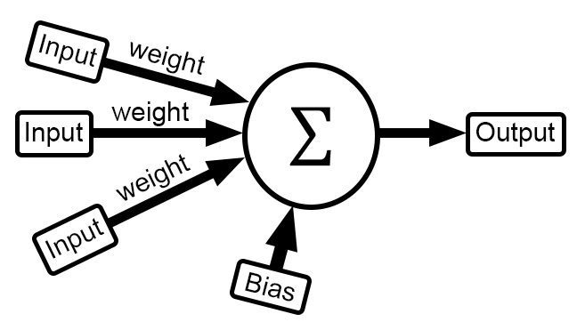
And now we get to the really interesting part, which is directly related to what we need to do in the code. When you look at the sum of the products of each input x and its weight w, you might not realize that this is a matrix operation. "How? I don't understand." Don't worry, dear reader; let's rewrite the sum in a clearer form so you can understand it. Let's take a look at this in the next image.

Now we have something truly beautiful before us. Although it is difficult to implement what is on the left in code, it is very easy to implement what is on the right. This is because we can use arrays. This way, we can change the number of inputs to a neuron very easily and quickly. "That's just wonderful! How do I translate this into code?" Dear reader, below you can see what this looks like in the class code.
01. //+------------------------------------------------------------------+
02. #property copyright "Daniel Jose"
03. //+------------------------------------------------------------------+
04. #define macroRandom (rand() / (double)SHORT_MAX)
05. //+------------------------------------------------------------------+
06. class C_Neuron
07. {
08.     private:
09.         uint    m_Inputs;
10.         double  m_bias,
11.                 m_weight[];
12. //+------------------------------------------------------------------+
13.         inline double Cost(const double &train[])
14.         {
15.             double x, err;
16.
17.             err = 0;
18.             for (uint c0 = 0; c0 < train.Size(); c0++)
19.             {
20.                 x = 0;
21.                 for(uint c1 = 0; c1 < m_Inputs; c1++, c0++)
22.                    x += (train[c0] * m_weight[c1]);
23.                 err += MathPow((x + m_bias) - train[c0], 2);
24.             }
25.
26.             return err;
27.         }
28. //+------------------------------------------------------------------+
29.     public :
30. //+------------------------------------------------------------------+
31.         C_Neuron(const uint nInputs = 1, double H = 1.0, double L = 0.0)
32.         {
33.             MathSrand(512);
34.             m_Inputs = nInputs;
35.             ArrayResize(m_weight, m_Inputs);
36.             for(uint c = 0; c < m_Inputs; c++)
37.                 m_weight[c] = ((double)macroRandom * (H - L)) + L;
38.             m_bias = (double)macroRandom;
39.         }
40. //+------------------------------------------------------------------+
41.         ~C_Neuron()
42.         {
43.             ArrayFree(m_weight);
44.         }
45. //+------------------------------------------------------------------+
46.         void View_Variables(void)
47.         {
48.             Print("Bias: ", m_bias);
49.             for (uint c = 0, m = m_weight.Size(); c < m; c++)
50.                 PrintFormat("Weight[%d]: %.16f", c, m_weight[c]);
51.         }
52. //+------------------------------------------------------------------+
53.         inline double Learning(const double &train[], const double epsilon = 1e-3, const ulong limit = ULONG_MAX)
54.         {
55.             double  err,
56.                     mem_b,
57.                     err_w[],
58.                     mem_w[];
59.
60.             ArrayResize(err_w, m_Inputs);
61.             ArrayResize(mem_w, m_Inputs);
62.             for (ulong count = 0; (count < limit) && ((err = Cost(train)) > epsilon); count++)
63.             {
64.                 ArrayCopy(mem_w, m_weight);
65.                 for (uint c = 0, m = m_weight.Size(); c < m; c++)
66.                 {
67.                     m_weight[c] += epsilon;
68.                     err_w[c] = Cost(train) - err;
69.                     m_weight[c] = mem_w[c];
70.                 }
71.                 mem_b = m_bias;
72.                 m_bias += epsilon;
73.                 m_bias = mem_b - (Cost(train) - err);
74.                 for (uint c = 0, m = m_weight.Size(); c < m; c++)
75.                     m_weight[c] -= err_w[c];
76.             }
77.             ArrayFree(err_w);
78.             ArrayFree(mem_w);
79.
80.             return err;
81.         }
82. //+------------------------------------------------------------------+
83. };
84. //+------------------------------------------------------------------+
85. #undef macroRandom
86. //+------------------------------------------------------------------+
Due to some differences between C/C++ and MQL5, the code turned out somewhat different from the version that, in my opinion, would have been more readable. Still, it's not hard to understand. Here, we've implemented the very basics: this neuron will use the least squares method as its loss function and can have as many inputs as needed. There is one small detail that will significantly affect how you work with this class. We'll see that a little later.
Let's start by breaking down the code we've written. First, let's look at the class constructor, which is on line 31. Notice how simple, clear, and straightforward it is. Using its arguments, we can specify how many inputs the neuron will have. In addition, we can specify the upper and lower bounds of the pseudorandom values that will be assigned during initialization.
As you can see, we're now beginning to explore this topic in greater detail. On line 33, we specify how the pseudorandom number generator will be initialized. Since our purpose is educational, we will use a fixed value. In a real-world scenario, line 33 would be slightly different. In fact, that would be the only line in the entire class code that would need to be changed.
So, in the next few steps, we'll initialize the class's internal variables. First, let's store the number of inputs on line 34. Next, on line 35, we allocate enough memory for the weight array—one weight for each input. To initialize these weights, we use a loop on line 36. Finally, on line 38, we initialize the bias. At this point, our neuron will be ready for training.
Okay, on line 41 we have a destructor whose sole purpose is to free the memory reserved for storing the weights. Since our neuron can have multiple inputs and we might want to view their contents, line 46 contains a very simple but very useful procedure. Its sole purpose is to display the values of all the neuron's variables in the MetaTrader 5 terminal. On line 48, we specify that the bias value should be printed. Line 49 displays all the weights. In other words, we don't need to specify again how many inputs the neuron should display. Since it knows how many inputs it has, it will show us all of them. It’s straightforward, simple, and practical.
And now let's move on to the part you've all been waiting for: the functions used to train a neuron. First, we'll use a squared-error loss function. Since it requires more computational power, we will soon replace it with a different type—most likely some gradient-based method. Let's leave that for later. First, let's take a look at how the least squares method works.
First and foremost, dear reader, you need to understand this: it doesn't matter where you use this neuron. If a neuron can interpret the training data, you can use it without understanding exactly what type of function is used for training. This might sound a little abstract. Since we're using a class, we can change anything within it without notifying the code that uses it of these internal changes. This way, we can use a more efficient loss function without the application that uses this class needing to be aware of it. This is very convenient, since we can switch to gradient-based training without notifying the application that uses this class.
To do this, we need a suitable interface. For this reason, the only function we will use for training is the one declared on line 53. Please note that it is quite simple and requires only a few arguments. The first one contains training data. The second specifies the target error value; once this value is reached, training is considered complete. The last argument specifies the number of iterations allowed. This argument allows us to evaluate the training and determine whether it converges to a solution. As shown in previous articles, it may happen that a neuron—or, more precisely, the function we are looking for—is unable to converge to a solution.
Inside this function, declared on line 53, we declare several local variables on line 55. On lines 60 and 61, we allocate memory for temporary use. On line 62, we enter a loop that will repeat a specified number of times. We have already explained this loop in other articles, although its contents differ slightly. Please note that on line 64, we copy the weights to a temporary memory area. It's not very efficient, but it'll do for our purposes for now.
On line 65, we enter a new inner loop that iterates through the inputs one by one and calculates the error values for each input. The new error values for each input are temporarily stored in memory, as shown on line 68. After calculating the errors for all inputs based on the desired change, we must adjust the bias error value. This is done on line 73. Finally, we can use the loop on line 74 to adjust each weight based on the error calculated earlier.
After all of this is done, the code returns to line 62, where a new iteration begins. The loop will continue until the specified iteration limit or target error value is reached. As soon as either of these two conditions is met, the loop will end, and lines 77 and 78 will be executed to free the allocated memory. Since this can sometimes be useful, in line 80 we'll return the error value obtained during training. That way, we'll be able to check whether it falls within the expected range when we test the training with a small number of iterations.
All right, let's move on to line 13. As you can see, in this training function, we call the function that calculates the error several times. As can be seen in line 13, this function takes one argument. Since this is an array, we can pass much more information than we could with a different type of structure. We need to be a little careful here. Please pay close attention, dear reader, because if you don't understand what I'm about to explain, you'll run into problems when trying to train a neuron with more or fewer inputs.
Let's not rush things. On line 18, we start a loop that will iterate through the entire array. As you can see, this pass does not distinguish between the different kinds of values. In other words, the function will never check whether a value represents an input or a target value. However, if you do everything right, you won't have any problems. Let's take a look at how to avoid them when working with this array.
When creating a neuron, we specify how many inputs it should have. When the loop in line 21 is executed, the loss function will take each value from the training array and multiply it by the weight of the corresponding input. This is part of the matrix calculations. We multiply the values and add each product to the previous result. Both the training array and the weight array are one-dimensional. The dot product of the inputs and their weights yields a scalar value. A bias is then added to this value, and the result is subtracted from the target value.
After calculating this result, we square it and add it to the previous values. Thus, we obtain the sum of squared errors. What I just explained is carried out on line 23. After looping through the training values, we return the total error calculated on line 26.
If you look at this loss function and pay attention to what's happening in the loops, it might seem a little strange to you, and you might think it won't work. Let's test this using the code below.
01. //+------------------------------------------------------------------+
02. #property copyright "Daniel Jose"
03. //+------------------------------------------------------------------+
04. #include <Neural Network\C_Neuron.mqh>
05. //+------------------------------------------------------------------+
06. double Train[] {
07.                 0, 0,
08.                 1, 2,
09.                 2, 4,
10.                 3, 6,
11.                 4, 8
12.                };
13. //+------------------------------------------------------------------+
14. void OnStart()
15. {
16.     C_Neuron *neuron;
17.
18.     Print("************************************");
19.     Print("Simple Neuron in Class...");
20.
21.     neuron = new C_Neuron(1);
22.
23.     (*neuron).View_Variables();
24.     Print("********** RESULT *************");
25.     Print("Error: ", (*neuron).Learning(Train));
26.     (*neuron).View_Variables();
27.
28.     delete neuron;
29. }
30. //+------------------------------------------------------------------+
The result of running the code is shown in the following image.
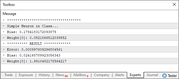
Please note that the result is within the expected range, which indicates that the neuron is functioning correctly. Wait a minute: how does the code we just looked at work? That looks a little strange. Dear reader, as I mentioned earlier, everything we’ll be doing here will be explained as clearly as possible. There are two points in this code that you should keep in mind when using the neuron class. First, there is the training data, which must be prepared based on the number of inputs to the neuron. These two things are closely related. If you change one without taking the other into account, you'll make a mistake or end up with a completely disoriented neuron that won't know what to do with the data.
Take note of this. The training data is specified on the sixth line. Here, the training data is prepared for a neuron with a single input. For this reason, in line 21, we specify that the neuron will have one input. Let's get back to the training data. Please note that I've organized the array so that it looks like a matrix with two columns and several rows. To keep the data organized, I recommend arranging it in an array like this.
In other words, you need one column for each input to the neuron, plus a final column containing the target value, or an estimate if the exact value is unknown. To make it clearer: if you want a neuron to have two inputs, you need to organize the array into three columns. The third will contain a value that allows the neuron to assess how far off it is. This will allow it to adjust the value of the loss function and, in this way, learn.
For now, it's best to take things slowly with this neuron, since it may reach a plateau that will prevent it from making progress in training. This is because it lacks an activation function.
You can see how this happens in the article "Neural Networks in Practice: Practice Makes Perfect", where I demonstrated that a neuron can be used to represent a logic gate. Since the neuron lacked an activation function, it would occasionally reach a plateau where its learning slowed significantly or stopped altogether.
Remember that we're just beginning a new phase, during which I'll explain various things to you. For now, we already have a starting point for our study. Nevertheless, this neuron can be used to solve some simple polynomial problems. For example, if you modify the code to use a different set of training data, you'll see that it still generates quite acceptable results, even if they aren't exact. It will all depend on whether the equation used to generate the data can be expressed as a linear or affine function. For example, let's modify the code as shown below.
01. //+------------------------------------------------------------------+
02. #property copyright "Daniel Jose"
03. //+------------------------------------------------------------------+
04. #include <Neural Network\C_Neuron.mqh>
05. //+------------------------------------------------------------------+
06. double Train[] {
07.                   1,    3,  10.35  ,
08.                 1.5,  3.25, 11.7875,
09.                 1.75, 3.94, 13.721 ,
10.                 2.85, 3.46, 14.669 ,
11.                };
12. //+------------------------------------------------------------------+
13. void OnStart()
14. {
15.     C_Neuron *neuron;
16.
17.     Print("************************************");
18.     Print("Simple Neuron in Class...");
19.
20.     neuron = new C_Neuron(2);
21.
22.     (*neuron).View_Variables();
23.     Print("********** RESULT *************");
24.     Print("Error: ", (*neuron).Learning(Train));
25.     (*neuron).View_Variables();
26.
27.     delete neuron;
28. }
29. //+------------------------------------------------------------------+
Now we see something a little different. Line 6 contains new training data prepared for a neuron with two inputs instead of one. When we run this new code, we get the result shown in the following image.
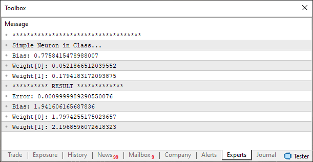
Simple, isn't it? Dear reader, remember what we discussed earlier: we need to prepare and check the training data array, keeping in mind that each column represents a single input. The last column will contain values that allow the neuron to estimate its error based on the values of its internal parameters—weights and bias—which are initialized pseudorandomly. In this second training example, the data is arranged in three columns. We therefore need to change the value on line 20 from “1” to “2”. In this way, the neuron will be able to interpret the two values as inputs and use the third as the target value to correct the error at each iteration.
Since the entire code is designed so that we don't have to modify it, the neuron will automatically allocate enough space to analyze two inputs. So, we finally have an implementation that eliminates the need to write or modify code every time we need to change the number of a neuron's inputs.
Concluding Thoughts
In this article, we begin to move away from the previous approach to programming, in which every change, adjustment, or new requirement for a neuron forced us to modify the code. Now we are beginning to encapsulate the implementation so that it can be used, improved, and modified without much difficulty. As new features are added to the neuron, any code that uses this class will benefit from these changes.
So far, we have created the simplest implementation of all: the neuron still uses a loss function based on the least squares method and does not yet have an activation function. In addition, we are missing one more element, which we will implement later: a backpropagation mechanism that allows an error to be propagated among several connected neurons. The current mechanism is limited to a single neuron. For more complex training, we need to improve this mechanism so that we can connect neurons in a cascade. In other words, dear reader, we need to create a backpropagation mechanism capable of propagating an error when neurons are connected one after another. With the current mechanism, if you try to do this and create a small neural network, at some point it will get stuck and be unable to continue training.
As I mentioned earlier, we'll look at how to do this later. In the meantime, start studying the code in this article and experimenting with it. In the attached file, you'll find the two neurons we discussed here, as well as the original class. See you in the next article.
| MQ5 File | Description |
|---|---|
| Scripts\Example A | Basic Demonstration |
| Scripts\Example B | Basic Demonstration |
Translated from Portuguese by MetaQuotes Ltd.
Original article: https://www.mql5.com/pt/articles/13873
Warning: All rights to these materials are reserved by MetaQuotes Ltd. Copying or reprinting of these materials in whole or in part is prohibited.
This article was written by a user of the site and reflects their personal views. MetaQuotes Ltd is not responsible for the accuracy of the information presented, nor for any consequences resulting from the use of the solutions, strategies or recommendations described.