Neural Network in Practice: Least Squares

Introduction
Hello everyone and welcome to a new article about neural networks.
In the previous article Neural Network in Practice: Secant Line, we began to discuss applied mathematics in practice. However, this was only a short and quick introduction to the topic. We have seen that the basic mathematical operation to be used is the trigonometric function. And, contrary to what many think, this is not a tangent function but a secant function. Although this may all seem quite confusing at first, you will soon find that everything is much simpler than it seems. Unlike many people who only create a lot of confusion in the mathematical environment, here everything develops completely naturally.
Something strange and incomprehensible
However, there is one small flaw, which I could not understand. It makes no sense, at least for me. Since this might be useful for anyone who tries to do the same, I left it as is. We will fix this problem here because if we don't fix it, we will have many other problems from the mathematical side.
The article mentioned above has the following code:
19. //+------------------------------------------------------------------+
20. void Func_01(void)
21. {
22.     int A[] {
23.                 -100,  150,
24.                  -80,   50,
25.                   30,  -80,
26.                  100, -120
27.             };
28.
29.     canvas.LineVertical(global.x, global.y - _SizeLine, global.y + _SizeLine, ColorToARGB(clrRoyalBlue, 255));
30.     canvas.LineHorizontal(global.x - _SizeLine, global.x + _SizeLine, global.y, ColorToARGB(clrRoyalBlue, 255));
31.
32.     for (uint c0 = 0, c1 = 0; c1 < A.Size(); c0++)
33.         canvas.FillCircle(global.x + A[c1++], global.y + A[c1++], 5, ColorToARGB(clrRed, 255));
34. }
35. //+------------------------------------------------------------------+
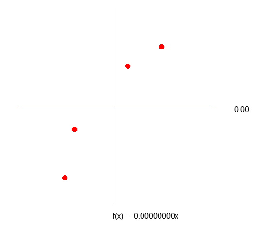
This code constructs small circles whose position is in array A shown in line 22. Nothing special yet, that's exactly how it was intended. However, when plotting the points, we get the following:
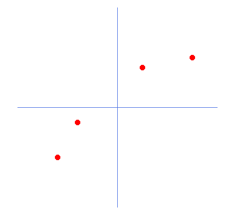
These points are in the wrong places. They are inverted with respect to the X and Y axes. Why? Honestly, I don't know how to explain this. This happens because in line 33 of the code we capture the values that are in the array and then add the position. This way the compiler should understand that we are pointing to the next value in the array. This is exactly how it happens, and if it were different, an unauthorized memory access error would be generated. This would be treated as a range error, and the application would terminate.
However, in global.x, odd index values are added, not even ones. Thus, the values added to global.y are at an even index, whereas they would be expected to be at an odd index.
I only realized this when I started writing the math for this article, because the calculations didn't match the results the app provided. So I decided to find the reason. You can do the same by slightly modifying the code as shown below.
19. //+------------------------------------------------------------------+
20. void Func_01(void)
21. {
22.     int A[]={
23.                 -100,  150,
24.                  -80,   50,
25.                   30,  -80,
26.                  100, -120
27.             };
28.
29.     int vx, vy;
30.     string s = "";
31.
32.     canvas.LineVertical(global.x, global.y - _SizeLine, global.y + _SizeLine, ColorToARGB(clrRoyalBlue, 255));
33.     canvas.LineHorizontal(global.x - _SizeLine, global.x + _SizeLine, global.y, ColorToARGB(clrRoyalBlue, 255));
34.
35.     for (uint c0 = 0, c1 = 0; c1 < A.Size(); c0++)
36.     {
37.         canvas.FillCircle(global.x + (vx = A[c1++]), global.y + (vy = A[c1++]), 5, ColorToARGB(clrRed, 255));
38.         s += StringFormat("[ %d <> %d ] ", vx, vy);
39.     }
40.     canvas.TextOut(global.x - 200, global.y + _SizeLine + 70, s, ColorToARGB(clrBlack));
41. }
42. //+------------------------------------------------------------------+
This modification allows us to see what is happening. The result is shown below:
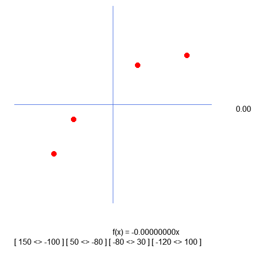
Note the values inside the brackets. They are the result of the capture performed in line 37. That is, we fix the values that are used to position the circles on the graph. However, note that they are inverted compared to what is declared in the array. And this is quite strange. Therefore, we need to change the code as shown below.
19. //+------------------------------------------------------------------+
20. void Func_01(void)
21. {
22.     int A[]={
23.                 -100,  150,
24.                  -80,   50,
25.                   30,  -80,
26.                  100, -120
27.             };
28.
29.     int vx, vy;
30.     string s = "";
31.
32.     canvas.LineVertical(global.x, global.y - _SizeLine, global.y + _SizeLine, ColorToARGB(clrRoyalBlue, 255));
33.     canvas.LineHorizontal(global.x - _SizeLine, global.x + _SizeLine, global.y, ColorToARGB(clrRoyalBlue, 255));
34.
35.     for (uint c0 = 0, c1 = 0; c1 < A.Size(); c0++)
36.     {
37.         vx = A[c1++];
38.         vy = A[c1++];
39.         canvas.FillCircle(global.x + vx, global.y + vy, 5, ColorToARGB(clrRed, 255));
40.         s += StringFormat("[ %d <> %d ] ", vx, vy);
41.     }
42.     canvas.TextOut(global.x - 200, global.y + _SizeLine + 70, s, ColorToARGB(clrBlack));
43. }
44. //+------------------------------------------------------------------+
Now when we use this new code, the result will look like this:
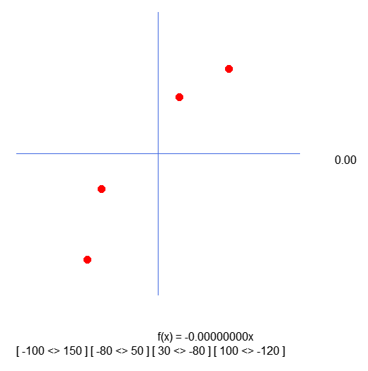
You can see that the values inside the square brackets correspond to what is declared in the array. I apologize for not noticing this error earlier. But let this serve as a warning to all those who want to do things their own way. Since I didn't understand why the indices were reversed, I don't know how to explain its. Having made this fix that is really necessary, we can move on to further work.
Preparing to do math and more math
What we do from this point on can be quite confusing if you just dive into the code. Since I want you to understand exactly what we are going to do and why, I will explain everything calmly. Therefore, I recommend reading carefully. Change the code as it appears. Try to understand what is happening. Only when you understand everything, move on to the next step. Don't try to skip steps because you might not understand anything at all.
The first thing that we will do is slightly change the code.
19. //+------------------------------------------------------------------+
20. void Func_01(void)
21. {
22.     int A[]={
23.                 -100,  150,
24.                  -80,   50,
25.                   30,  -80,
26.                  100, -120
27.             };
28.
29.     int vx, vy;
30.     string s = "";
31.     double ly;
32.
33.     canvas.LineVertical(global.x, global.y - _SizeLine, global.y + _SizeLine, ColorToARGB(clrRoyalBlue, 255));
34.     canvas.LineHorizontal(global.x - _SizeLine, global.x + _SizeLine, global.y, ColorToARGB(clrRoyalBlue, 255));
35.
36.     for (uint c0 = 0, c1 = 0; c1 < A.Size(); c0++)
37.     {
38.         vx = A[c1++];
39.         vy = A[c1++];
40.         canvas.FillCircle(global.x + vx, global.y + vy, 5, ColorToARGB(clrRed, 255));
41.         ly = (vx * MathTan(_ToRadians(global.Angle))) - vy;
42.         canvas.LineVertical(global.x + vx, global.y + vy, global.y + (int)(ly + vy), ColorToARGB(clrPurple));
43.         s += StringFormat("sy%d = %.4f  | ", c0, ly);
44.     }
45.     canvas.TextOut(global.x - 200, global.y + _SizeLine + 50, s, ColorToARGB(clrBlack));
46. }
47. //+------------------------------------------------------------------+
48. void NewAngle(const char direct, const double step = 0.2)
49. {
50.     canvas.Erase(ColorToARGB(clrWhite, 255));
51.
52.     global.Angle = (MathAbs(global.Angle + (step * direct)) < 90 ? global.Angle + (step * direct) : global.Angle);
53.     canvas.TextOut(global.x + _SizeLine + 50, global.y, StringFormat("%.2f", MathAbs(global.Angle)), ColorToARGB(clrBlack));
54.     canvas.TextOut(global.x, global.y + _SizeLine + 20, StringFormat("f(x) = %.8fx", -MathTan(_ToRadians(global.Angle))), ColorToARGB(clrBlack));
55.     canvas.Line(
56.                 global.x - (int)(_SizeLine * cos(_ToRadians(global.Angle))),
57.                 global.y - (int)(_SizeLine * sin(_ToRadians(global.Angle))),
58.                 global.x + (int)(_SizeLine * cos(_ToRadians(global.Angle))),
59.                 global.y + (int)(_SizeLine * sin(_ToRadians(global.Angle))),
60.                 ColorToARGB(clrForestGreen)
61.             );
62.
63.     Func_01();
64.
65.     canvas.Update(true);
66. }
67. //+------------------------------------------------------------------+
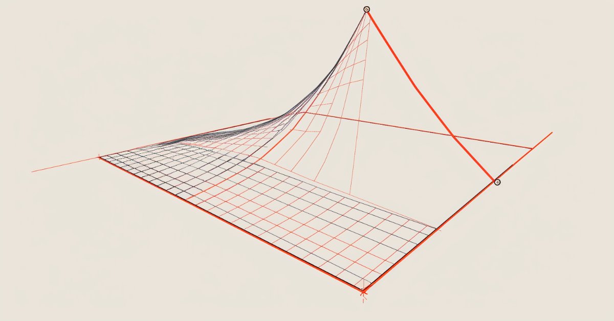
Although this is not the most optimal way, the result shown in the animation below is exactly what we want to visualize:
We just create a purple line. It indicates the distance between the line and the point. Please pay attention to this. The length of the line is determined by code in line 41 of the fragment. The calculation is not quite as it should be, but it works. So let's not rush, because later we will need to change this calculation. In line 43, we create a text string that allows us to find out the length of the given purple line. Look at the animation, and you will see that there are negative lengths, which does not make sense. It's too early to worry about it. First of all, I want you to understand the essence of our work.
Now, I want you, dear reader, to think a little. The straight line function is calculated based on the slope coefficient. This coefficient can be obtained from the angle, which we change by clicking on the arrows to the right or left. And the rate at which this slope changes is specified by the 'step' value present in line 52.
Then look at the length of each of the purple lines. With a little patience, we can make the slope of the straight line as steep as possible so that the length of each of the purple lines stops increasing (it can decrease, but it should not increase). When we get to the point where none of the lengths grow, we have found the ideal slope.
But note the following: In this case, we only need to consider four elements, which is quite simple. However, if there were hundreds or thousands of points in the array, manually adjusting the values so that they did not increase would be very difficult. We can use a mathematical trick to simplify this process. The trick is this: If we add up the lengths of each of the purple lines, we only need to watch one value, and if it starts to go up, we know we've passed the optimal slope point. Simple, isn't it? So, let's change the code as follows.
19. //+------------------------------------------------------------------+
20. void Func_01(void)
21. {
22.     int A[]={
23.                 -100,  150,
24.                  -80,   50,
25.                   30,  -80,
26.                  100, -120
27.             };
28.
29.     int vx, vy;
30.     double ly, err;
31.
32.     canvas.LineVertical(global.x, global.y - _SizeLine, global.y + _SizeLine, ColorToARGB(clrRoyalBlue, 255));
33.     canvas.LineHorizontal(global.x - _SizeLine, global.x + _SizeLine, global.y, ColorToARGB(clrRoyalBlue, 255));
34.
35.     err = 0;
36.     for (uint c0 = 0, c1 = 0; c1 < A.Size(); c0++)
37.     {
38.         vx = A[c1++];
39.         vy = A[c1++];
40.         canvas.FillCircle(global.x + vx, global.y + vy, 5, ColorToARGB(clrRed, 255));
41.         ly = (vx * MathTan(_ToRadians(global.Angle))) - vy;
42.         canvas.LineVertical(global.x + vx, global.y + vy, global.y + (int)(ly + vy), ColorToARGB(clrPurple));
43.         err += MathAbs(ly);
44.     }
45.     canvas.TextOut(global.x - 200, global.y + _SizeLine + 20, StringFormat("Error: %.8f", err), ColorToARGB(clrRed));
46. }
47. //+------------------------------------------------------------------+
The result can be seen in gif below. Adjusting the values this way is much easier.
Adjusting the quadrant
Before we fully dive into the math side, we need to make a small modification. While it won't directly affect what we're going to do, it will be relevant if we decide to apply what's been explained in other programs, or when experimenting manually. Often we start by trying everything manually, doing the calculations in the same way. The following will help you avoid the mistake when blindly relying on the program's calculations.
Even if they are completely wrong. Beginner programmers often make this mistake, and it can cost a lot of time and effort. As a result, they focus on solving the problem in the wrong way. Every good programmer is also a person who is very suspicious of the calculations being made. The programmer always seeks to test different things in a lot of different ways before finally trusting the result.
I tell you this because, although many people ignore this, when we create a graphic image, we are always working in the fourth quadrant of the Cartesian plane. This influences everything. Not on the calculations themselves, but on those who want to perform the same calculations manually or in another program. For example, MatLab, SCILab or even good old Excel. In Excel, for example, we can create a graphical representation of the values and formulas we use here.
That's good, but what does all this have to do with what we're going to do? Well, dear reader, if you look at the data matrix that is in the program, you will notice that it is a little strange compared to what is presented on the graph. If we plot the same values in another graphing program, we will see that the Y axis is inverted. But I still don't understand how this happens. Take your time and look at the images below to understand better.
The image above can be seen when plotting a chart in MetaTrader 5. However, when plotting the same values, for example, in Excel, the graph will look like this:

This mismatch can result in most of the tests that need to be performed being completely incomprehensible. Especially if you need to check whether the calculations are performed correctly.
In the previous topic we already figured out how to correctly present data. Now we need to fix this problem. The thing is that the Y axis is inverted (or mirrored).
Why does this failure in representation happen?! The reason is simple, and we mentioned it at the very beginning of the topic. The screen we plot the data on is in the fourth quadrant. This is because the origin, that is, the point (0, 0), is in the upper left corner. Now pay attention to the following. Even if we change the reference point to the center of the screen, this transfer will only be virtual. This means that we do not change the physical reference point. We are simply moving the representation of computation to a different starting point. For this reason, in the program we add the values of a point in the matrix to another set of points. This allows us to move the virtual origin from the upper left corner to any other place on the screen.
But you may have noticed in the image above that there is a problem with how we implement this virtualization. The Y axis is inverted or mirrored. To fix this, we need to change a few things in the code. It's simple, but it will make everything much clearer.
In the code, we will make the following changes:
19. //+------------------------------------------------------------------+
20. void Func_01(void)
21. {
22.     int A[]={
23.                 -100, -150,
24.                  -80,  -50,
25.                   30,   80,
26.                  100,  120
27.             };
28.
29.     int vx, vy;
30.     double ly, err;
31.
32.     canvas.LineVertical(global.x, global.y - _SizeLine, global.y + _SizeLine, ColorToARGB(clrRoyalBlue, 255));
33.     canvas.LineHorizontal(global.x - _SizeLine, global.x + _SizeLine, global.y, ColorToARGB(clrRoyalBlue, 255));
34.
35.     err = 0;
36.     for (uint c0 = 0, c1 = 0; c1 < A.Size(); c0++)
37.     {
38.         vx = A[c1++];
39.         vy = A[c1++];
40.         canvas.FillCircle(global.x + vx, global.y - vy, 5, ColorToARGB(clrRed, 255));
41.         ly = vy - (vx * -MathTan(_ToRadians(global.Angle)));
42.         canvas.LineVertical(global.x + vx, global.y - vy, global.y - (int)(ly + vy), ColorToARGB(clrPurple));
43.         err += MathAbs(ly);
44.     }
45.     canvas.TextOut(global.x - 200, global.y + _SizeLine + 20, StringFormat("Error: %.8f", err), ColorToARGB(clrRed));
46. }
47. //+------------------------------------------------------------------+
Please note that the changes are very subtle. First we change the values in the matrix. Then we change the calculation in line 40 so that the points are positioned correctly. It is also necessary to change lines 41 and 42, which perform computations to correctly connect the purple lines to the points. This type of fix, even if it is mainly aesthetic in nature, gives confidence to those who want to conduct a more in-depth study of the issue. Now we can compare generated graphs without thinking that something was poorly calculated in one or the other program. The process has become much easier.
As a result, the implementation of the task is now also much easier. Because if the error value increases, it means we are moving in the wrong direction. If it decreases, then we are moving in the right direction.
But now another question arises, and from this point we will begin to delve into what drives the topic of neural networks. Adjusting the slope of the tangent line or slope factor is fairly simple if you look at the error value. But is there a way to set it up automatically? Is it possible to create a mechanism that allows the machine to search for the best value of the coefficient. It is important to remember that we are now using only one variable in the system, since the tangent line passes exactly through the point (0, 0), which is the beginning of the Cartesian plane. But this is not always the case. However, let's resolve this simpler question first. This is the case where we only need to adjust one variable.
If you followed the previous article, you know that I mentioned how to calculate a secant line so that it becomes a tangent. Even if that works, let's think of another hypothesis, a little simpler, in which we don't have to go through so much trouble to find the value of the slope. Let's try to find a formula so that the coefficient can be calculated faster and easier.
To do this we need to apply some mathematical tricks. For greater clarity of presentation, we will consider this in a new topic.
Looking for the smallest area possible
If you have ever been trying to study the topic of artificial intelligence, you might gave noticed that there's something that keeps coming up. But do not confuse artificial intelligence with neural networks. Although these two concepts are correlated, they need to be approached differently. This is from a programming point of view. There are a few small differences, but here I intend to create a neural network that can find an equation that best represents the values in the database. This type of computation is performed by a neural network. Artificial intelligence searches at the basis. The neural network creates the basis.
In this case, we can start using neurons for this, but in my opinion, it is still too early. We can create calculations for this ourselves, which will save a huge amount of time on processing.
In order to calculate or create a calculation to find the slope, we will use derivatives. We could implement this in another way, but here we will use derivatives, which is the fastest way. I will assume that you have understood everything that was explained in the previous topic so that we can move on. Now let's move on to the mathematical part of the question.
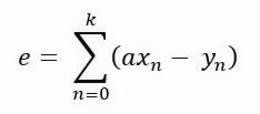
To find the error, we will perform the following mathematical computation.
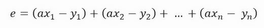
The value of the constant <a> in the formula is precisely the angular coefficient of the straight line, that is, it is the value of the tangent line that is created. But this formula is not compact enough. We can simplify it by making the formula a little more compact, as shown below.
Although they look like different formulas, they represent the same thing, only the notation has been changed to be more compact. Since it is more compact, writing the formulas we will develop below will be easier. Notice that at each step we have a sum of values, which is the length of the purple line in the graph shown in the previous topic. These things prevent us from using derivatives, because if we try to derive such a formulation, we will end up with a zero constant. We want to get the result presented in the formula below.
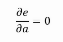
So we want to output the error relative to the slope of the straight line, and as that value approaches zero, the slope gets closer and closer to the ideal value. This is the idea. But this value can hardly be zero. It can approach zero, and the closer to it the better, but as I said, we cannot derive a function that determines the length of the purple line. Nevertheless, there is a way. We need to transform the purple line into a square figure, and in this case we are not looking for the minimum length of the line, but the smallest possible area of the square formed by each of the lines. Thus, we obtain the new formulation presented below.

Notice that now (although it doesn't look like it) we are computing the same coefficient, only this time using the area of the square formed by each of the purple lines on the graph. Things are getting a lot more interesting. If we develop this equation further, we get what is shown below.
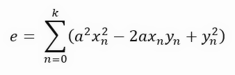
You might not have understood what we just did. This equation, which appeared simply by changing the calculation from the length of a line to the area of a square, is actually a very interesting equation. Do you see this? Can you tell me what this equation is?
If you can't figure out what this equation is, don't worry. This is nothing more than a quadratic equation. This is the same equation that generates the parabola, and therefore it is the equation that allows us to create the first-degree derivative. We want to get the derivative with respect to the slope. But before that, I'll add one more step that we don't usually take. I want to show you why the final formula looks like this. This additional step involves grouping the terms and separating them accordingly as shown below.
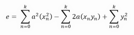
We have simplified the equation to make it easier to understand when we come to derivation. Typically this extra step is not performed; we go straight to the final formula shown below.

Sweet mother of God! Now everything has become very complicated. I don't understand anything at all, how is this possible? What kind of crazy calculations are these? How can I implement all this in code?! Everything is under control. Keep calm. I usually don't like to show formulas so as not to confuse the reader. And at the same time, everything is very simple: this is precisely the derivative that we need to calculate. Thus, we get an approximate value of the angular coefficient of the line.
Let's now translate this into code format and see what happens. The code is as follows.
19. //+------------------------------------------------------------------+
20. void Func_01(void)
21. {
22.     int A[]={
23.                 -100, -150,
24.                  -80,  -50,
25.                   30,   80,
26.                  100,  120
27.             };
28.
29.     int vx, vy;
30.     double ly, err, d0, d1;
31.
32.     canvas.LineVertical(global.x, global.y - _SizeLine, global.y + _SizeLine, ColorToARGB(clrRoyalBlue, 255));
33.     canvas.LineHorizontal(global.x - _SizeLine, global.x + _SizeLine, global.y, ColorToARGB(clrRoyalBlue, 255));
34.
35.     err = d0 = d1 = 0;
36.     for (uint c0 = 0, c1 = 0; c1 < A.Size(); c0++)
37.     {
38.         vx = A[c1++];
39.         vy = A[c1++];
40.         d0 += (vx * vy);
41.         d1 += MathPow(vx, 2);
42.         canvas.FillCircle(global.x + vx, global.y - vy, 5, ColorToARGB(clrRed, 255));
43.         ly = vy - (vx * -MathTan(_ToRadians(global.Angle)));
44.         canvas.LineVertical(global.x + vx, global.y - vy, global.y - (int)(ly + vy), ColorToARGB(clrPurple));
45.         err += MathAbs(ly);
46.     }
47.     canvas.TextOut(global.x - 200, global.y + _SizeLine + 20, StringFormat("Error: %.8f", err), ColorToARGB(clrRed));
48.     canvas.TextOut(global.x - 200, global.y + _SizeLine + 40, StringFormat("(de/da) : %.8f", d0 / d1), ColorToARGB(clrForestGreen));
49. }
50. //+------------------------------------------------------------------+
Note that, unlike what you might imagine from looking at all these formulas, doing the actual calculations in the code is quite simple and straightforward. In line 40 we calculate the sum of the points. In line 41 we calculate the square of the points in X. It's all very simple. In line 48 we print the value of the graph. Now pay close attention to what I am saying: This value we find is ideal when we take only a single variable in the equation of the line. Look at the formula of the equation of the line below.
In this equation, the value < a > is precisely the angular coefficient. The value < b > indicates the point where the root of the equation is located. For those who don't know, the roots of an equation are the points at which a curve or straight line (in this case) touches the Y-axis when the X value is zero. Then, since the value of < b > in this solution is zero, the value returned as the ideal value merely shows what should be the slope closest to the ideal. But that doesn't mean it's actually correct, because we're saying that the root of the equation is exactly at the origin, meaning X and Y are zero. In reality, this happens rarely, so rarely that when we run this application, we get the animation shown below.
Notice there is another line in this animation. It is only needed to show where the calculated ideal value will be. But if you look at the error value, you can see that the coefficient in the equation is slightly different from what is shown in green.
This green value exactly corresponds to the one we calculated based on the equation. It can be seen that simply calculating the value of the slope is not enough here. We need the equation of the line we are creating, and for this, in addition to the value < a >, we also need to get the value < b >. This is necessary in order to have a more general solution and not be tied to the point (0, 0).
This point (0, 0), which is not actually part of the database, has an implicit influence on the results of the calculations of the angular coefficient. To remove this point properly, we need to change a few things in the application so that you can move away from this reference point at (0, 0).
Moving the root of the line function
Since we need to prepare the application for further work (which will be discussed in the next article), we will create a rather interesting mechanism in the rest of this article. Then we can focus on the mathematical side.
Adding this mechanism does not require any special changes to the code. However, the effect will be quite significant, since it will allow us to find the line equation that will give us the smallest possible area in any situation. This will be a general mechanism for finding the most appropriate constants. With this mechanism, the linear regression that will be plotted on the graph will more adequately reflect the database.
Making these changes is very simple. All we need to do is move the root of the straight line function. These words seem a bit complicated, but when we implement the change in code, everything becomes quite simple as you can see below.
001. //+------------------------------------------------------------------+
002. #property copyright "Daniel Jose"
003. #property indicator_chart_window
004. #property indicator_plots 0
005. //+------------------------------------------------------------------+
006. #include <Canvas\Canvas.mqh>
007. //+------------------------------------------------------------------+
008. #define _ToRadians(A) (A * (M_PI / 180.0))
009. #define _SizeLine 200
010. //+------------------------------------------------------------------+
011. CCanvas canvas;
012. //+------------------------------------------------------------------+
013. struct st_00
014. {
015.     int     x,
016.             y;
017.     double  Angle,
018.             Const_B;
019. }global;
020. //+------------------------------------------------------------------+
021. void PlotText(const uchar line, const string sz0)
022. {
023.     uint w, h;
024.
025.     TextGetSize(sz0, w, h);
026.     canvas.TextOut(global.x - (w / 2), global.y + _SizeLine + (line * h) + 5, sz0, ColorToARGB(clrBlack));
027. }
028. //+------------------------------------------------------------------+
029. void Func_01(void)
030. {
031.     int A[]={
032.                 -100, -150,
033.                  -80,  -50,
034.                   30,   80,
035.                  100,  120
036.             };
037.
038.     int vx, vy;
039.     double ly, err;
040.     string s0 = "";
041.
042.     canvas.LineVertical(global.x, global.y - _SizeLine, global.y + _SizeLine, ColorToARGB(clrRoyalBlue, 255));
043.     canvas.LineHorizontal(global.x - _SizeLine, global.x + _SizeLine, global.y, ColorToARGB(clrRoyalBlue, 255));
044.
045.     err = 0;
046.     for (uint c0 = 0, c1 = 0; c1 < A.Size(); c0++)
047.     {
048.         vx = A[c1++];
049.         vy = A[c1++];
050.         canvas.FillCircle(global.x + vx, global.y - vy, 5, ColorToARGB(clrRed, 255));
051.         ly = vy - (vx * -MathTan(_ToRadians(global.Angle))) - global.Const_B;
052.         s0 += StringFormat("%.4f || ", MathAbs(ly));
053.         canvas.LineVertical(global.x + vx, global.y - vy, global.y + (int)(ly - vy), ColorToARGB(clrPurple));
054.         err += MathPow(ly, 2);
055.     }
056.     PlotText(3, StringFormat("Error: %.8f", err));
057.     PlotText(4, s0);
058. }
059. //+------------------------------------------------------------------+
060. void NewAngle(const char direct, const char updow, const double step = 0.1)
061. {
062.     canvas.Erase(ColorToARGB(clrWhite, 255));
063.
064.     global.Angle = (MathAbs(global.Angle + (step * direct)) < 90 ? global.Angle + (step * direct) : global.Angle);
065.     global.Const_B += (step * updow);
066.     PlotText(1, StringFormat("Angle in graus => %.2f", MathAbs(global.Angle)));
067.     PlotText(2, StringFormat("f(x) = %.4fx %c %.4f", -MathTan(_ToRadians(global.Angle)), (global.Const_B < 0 ? '-' : '+'), MathAbs(global.Const_B)));
068.     canvas.LineAA(
069.                 global.x - (int)(_SizeLine * cos(_ToRadians(global.Angle))),
070.                 (global.y - (int)global.Const_B) - (int)(_SizeLine * sin(_ToRadians(global.Angle))),
071.                 global.x + (int)(_SizeLine * cos(_ToRadians(global.Angle))),
072.                 (global.y - (int)global.Const_B) + (int)(_SizeLine * sin(_ToRadians(global.Angle))),
073.                 ColorToARGB(clrForestGreen)
074.             );
075.
076.     Func_01();
077.
078.     canvas.Update(true);
079. }
080. //+------------------------------------------------------------------+
081. int OnInit()
082. {
083.     global.Angle = 0;
084.     global.x = (int)ChartGetInteger(0, CHART_WIDTH_IN_PIXELS, 0);
085.     global.y = (int)ChartGetInteger(0, CHART_HEIGHT_IN_PIXELS, 0);
086.
087.     canvas.CreateBitmapLabel("BL", 0, 0, global.x, global.y, COLOR_FORMAT_ARGB_NORMALIZE);
088.     global.x /= 2;
089.     global.y /= 2;
090.
091.     NewAngle(0, 0);
092.
093.     canvas.Update(true);
094.
095.     return INIT_SUCCEEDED;
096. }
097. //+------------------------------------------------------------------+
098. int OnCalculate(const int rates_total, const int prev_calculated, const int begin, const double &price[])
099. {
100.     return rates_total;
101. }
102. //+------------------------------------------------------------------+
103. void OnChartEvent(const int id, const long &lparam, const double &dparam, const string &sparam)
104. {
105.     switch (id)
106.     {
107.         case CHARTEVENT_KEYDOWN:
108.             if (TerminalInfoInteger(TERMINAL_KEYSTATE_LEFT))
109.                 NewAngle(-1, 0);
110.             if (TerminalInfoInteger(TERMINAL_KEYSTATE_RIGHT))
111.                 NewAngle(1, 0);
112.             if (TerminalInfoInteger(TERMINAL_KEYSTATE_UP))
113.                 NewAngle(0, 1);
114.             if (TerminalInfoInteger(TERMINAL_KEYSTATE_DOWN))
115.                 NewAngle(0, -1);
116.             break;
117.     }
118. }
119. //+------------------------------------------------------------------+
120. void OnDeinit(const int reason)
121. {
122.     canvas.Destroy();
123. }
124. //+------------------------------------------------------------------+
Here are the results:
Essentially, to move the root, we have added a variable in line 18. Using the up and down arrows, we can change the value of this variable in line 65. Everything else is pretty simple. We just need to adjust the purple line length value based on the value of this new variable present in the code. I'm sure I don't need to explain how to do this because it's very simple.
Final considerations
In this article, we saw that mathematical formulas often look much more complicated than their implementation in code. Many people think that doing such things is difficult, but here we have shown that everything is much simpler than it seems. But we have not done all the work yet. We have only implemented part of it. Now we need to find a way to write the equation of a line in a more appropriate way. For this, we will use the last code from this article. Contrary to what you might have imagined at the beginning of this topic, finding a straight line function through a loop is not as easy as it seemed. This happens because we add another variable to search for. Just think how much work it would take to find an equation if we had a million variables. Doing this by brute force would be completely impossible, but with the right use of mathematics, finding the equation is much easier.
One last thing: Before you move on to the next article, use the code provided at the end, which generates what is shown in the image above, to try to find the equation. You will see that this is quite a difficult task. So see you in the next article.
Translated from Portuguese by MetaQuotes Ltd.
Original article: https://www.mql5.com/pt/articles/13670
Warning: All rights to these materials are reserved by MetaQuotes Ltd. Copying or reprinting of these materials in whole or in part is prohibited.
This article was written by a user of the site and reflects their personal views. MetaQuotes Ltd is not responsible for the accuracy of the information presented, nor for any consequences resulting from the use of the solutions, strategies or recommendations described.

- Free trading apps
- Over 8,000 signals for copying
- Economic news for exploring financial markets
You agree to website policy and terms of use