Neural Networks in Practice: Practice Makes Perfect

Introduction

Hello and welcome to another article about neural networks.

In the previous article,  Neural Networks in Practice: The First Neuron, we created our first neuron. However, programming is not that simple. Many people simply create, or rather copy, some code and start using it. This is definitely not a problem. By no means is there anything wrong with it; quite the opposite. It is a fairly sensible practice, provided, of course, that we study the code and try to improve it so that it meets our needs. What is wrong is using something without understanding how it works. Or, even worse, complaining about something or starting to talk about something we know absolutely nothing about.

Despite being functional, the code we examined in the previous article should under no circumstances be used in more complex applications. This is necessary so that everything is done in a timely manner or at least within certain expectations regarding the results.

So that you, dear readers, can understand what I am talking about, let us see how things look and what problems may arise if we make a few changes. But to make it clearer, let us look at this as a new topic.

Making Execution Time Unreasonably Long

Great, our simple and unique neuron can be seen in the following code.

01. //+------------------------------------------------------------------+
02. #property copyright "Daniel Jose"
03. //+------------------------------------------------------------------+
04. #define macroRandom (rand() / (double)SHORT_MAX)
05. #define macroSigmoid(a) (1.0 / (1 + MathExp(-a)))
06. //+------------------------------------------------------------------+
07. double Train[][3] {
08.                     {0, 0, 0},
09.                     {0, 1, 0},
10.                     {1, 0, 0},
11.                     {1, 1, 1},
12.                   };
13. //+------------------------------------------------------------------+
14. const uint nTrain = Train.Size() / 3;
15. const double eps = 1e-3;
16. //+------------------------------------------------------------------+
17. double Cost(const double w0, const double w1, const double b)
18. {
19.     double err;
20. 
21.     err = 0;
22.     for (uint c = 0; c < nTrain; c++)
23.         err += MathPow((macroSigmoid((Train[c][0] * w0) + (Train[c][1] * w1) + b) - Train[c][2]), 2);
24. 
25.     return err / nTrain;
26. }
27. //+------------------------------------------------------------------+
28. void OnStart()
29. {
30.     double  w0, w1, err, ew0, ew1, eb, bias;
31.     ulong count, it0, it1;
32. 
33.     Print("The Neuron - Tutor ...");
34.     MathSrand(512);
35.     w0 = (double)macroRandom;
36.     w1 = (double)macroRandom;
37.     bias = (double)macroRandom;
38. 
39.     it0 = GetTickCount();
40. 
41.     for (count = 0; (count < ULONG_MAX) && ((err = Cost(w0, w1, bias)) > eps); count++)
42.     {
43.         ew0 = (Cost(w0 + eps, w1, bias) - err) / eps;
44.         ew1 = (Cost(w0, w1 + eps, bias) - err) / eps;
45.         eb  = (Cost(w0, w1, bias + eps) - err) / eps;
46.         w0 -= (ew0 * eps);
47.         w1 -= (ew1 * eps);
48.         bias -= (eb * eps);
49.     }
50. 
51.     it1 = GetTickCount();
52.     Print("Time: ", (it1 - it0) / 1000.0, " seconds.");
53.     PrintFormat("%I64u > w0: %.4f %.4f || w1: %.4f %.4f || b: %.4f %.4f || %.4f", count, w0, ew0, w1, ew1, bias, eb, err);
54.     Print("w0 = ", w0, " || w1 = ", w1, " || Bias = ", bias);
55.     Print("Error Weight 0: ", ew0);
56.     Print("Error Weight 1: ", ew1);
57.     Print("Error Bias: ", eb);
58.     Print("Error: ", err);
59. 
60.     Print("Testing the neuron...");
61.     for (uchar p0 = 0; p0 < 2; p0++)
62.         for (uchar p1 = 0; p1 < 2; p1++)
63.             PrintFormat("%d AND %d IS %f", p0, p1, macroSigmoid((p0 * w0) + (p1 * w1) + bias));
64. 
65.     Print("************************************");
66. }
67. //+------------------------------------------------------------------+

We have made a few changes to the code compared to what was published in the previous article. The reason is quite simple. We want to show how a simple change can noticeably affect the overall execution time as well as the expected results. When the code above is run in MetaTrader 5, something very similar to this will be generated:

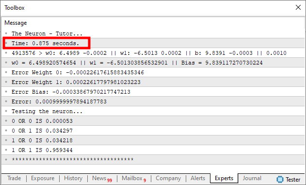
Pay attention to some of the data shown in the image above. The most obvious one, and the one we want to highlight, is, of course, the code execution time. This timing reflects only the part where we adjust the neuron's parameters. You can see this by looking at the code. Notice that in line 39 we capture the exact moment immediately before the neuron training process begins. In line 51, we capture the same kind of moment again, when training has finished. The difference between these two values gives us the training execution time. Please note that in line 52 we perform a small calculation. Since the captured time is measured in milliseconds, dividing the difference between the time values by one thousand gives us an approximate time in seconds. This is precisely the period highlighted in the image above.

Now let us see what we are going to do. In line 15 of the same code, we set the error to 0.001. But what will happen, in terms of execution time for this very same code, if we change the error to 0.0001, or 1e-4?

All right, try this on your own computer and see what happens. In any case, you will get something very similar to this:

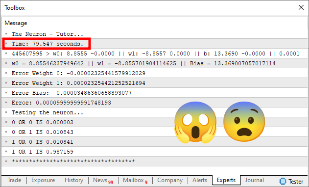
Now pay attention: simply changing the error from 1e-3 to 1e-4 makes the execution time increase from less than 1 second to almost 80 seconds. That is exactly what you are seeing. A simple tenfold change in precision caused the execution time to increase more than 80 times.

It is precisely moments like these that ultimately shatter the dreams of many beginners, especially those who have no idea that programming is by no means the easiest task. When we say that each program is often designed to perform a specific task, many people are surprised, especially when someone says that a neural network can do anything very quickly, although in reality this is not entirely true.

I would like to draw your attention to this fact, dear readers. Before moving on to adding new neurons to a network, it is extremely important to understand how the network will be built and for what purpose. To demonstrate this, we will take the very same simple neuron and replace it with something slightly different, while still intended to solve the same problem as in the code. In other words, we are going to make the neuron a bit more specialized — not in terms of fitting, but in terms of the number of inputs it is designed to handle. To separate these topics, let us discuss this in a separate section.

Adjusting the code to achieve better results

Now let us think about the following: what is the point of making a single neuron take 80 times longer just to improve precision by only 10 times? Such things make no sense. However, if we know in advance that throughout its lifetime the neuron will work with two inputs and one output, we can improve its code. This will speed up training and make the neuron more efficient at learning this specific task.

Making these changes may seem very difficult, as if only someone with extensive knowledge could accomplish such a feat. However, that is not quite true. All you need to understand, dear readers, is how the program works and what its purpose is. If you know this and understand how the program was written in a particular language, then you will be able, although it may take some time, to implement a much better solution.

To demonstrate this, we will modify the code from the previous topic while preserving the original code. Our goal is to understand whether we are moving in the right direction or not. A good programmer never tries to modify unknown code. First, they try to understand the code, figure out how it works, and then attempt to make some improvements. With these considerations in mind, the new code is shown below:

01. //+------------------------------------------------------------------+
02. #property copyright "Daniel Jose"
03. //+------------------------------------------------------------------+
04. #define macroRandom (rand() / (double)SHORT_MAX)
05. #define macroSigmoid(a) (1.0 / (1 + MathExp(-a)))
06. //+------------------------------------------------------------------+
07. #define def_Fast
08. //+------------------------------------------------------------------+
09. double Train[][3] {
10.                     {0, 0, 0},
11.                     {0, 1, 0},
12.                     {1, 0, 0},
13.                     {1, 1, 1},
14.                   };
15. //+------------------------------------------------------------------+
16. const uint nTrain = Train.Size() / 3;
17. const double eps = 1e-4;
18. //+------------------------------------------------------------------+
19. double Cost(const double w0, const double w1, const double b)
20. {
21.     double err;
22. 
23.     err = 0;
24.     for (uint c = 0; c < nTrain; c++)
25.         err += MathPow((macroSigmoid((Train[c][0] * w0) + (Train[c][1] * w1) + b) - Train[c][2]), 2);
26. 
27.     return err / nTrain;
28. }
29. //+------------------------------------------------------------------+
30. double Cost_2(double &w0, double &w1, double &b)
31. {
32.     double err, ew0, ew1, eb;
33. 
34.     err = ew0 = ew1 = eb = 0;
35.     for (uint c = 0; c < nTrain; c++)
36.     {
37.         err += MathPow((macroSigmoid((Train[c][0] * w0) + (Train[c][1] * w1) + b) - Train[c][2]), 2);
38.         ew0 += MathPow((macroSigmoid((Train[c][0] * (w0 + eps)) + (Train[c][1] * w1) + b) - Train[c][2]), 2);
39.         ew1 += MathPow((macroSigmoid((Train[c][0] * w0) + (Train[c][1] * (w1 + eps)) + b) - Train[c][2]), 2);
40.         eb += MathPow((macroSigmoid((Train[c][0] * w0) + (Train[c][1] * w1) + (b + eps)) - Train[c][2]), 2);
41.     }
42. 
43.     w0 -= (((ew0 - err)/ eps) * eps);
44.     w1 -= (((ew1 - err)/ eps) * eps);
45.     b  -= (((eb - err)/ eps) * eps);
46. 
47.     return err / nTrain;
48. }
49. //+------------------------------------------------------------------+
50. void OnStart()
51. {
52.     double  w0, w1, err, ew0, ew1, eb, bias;
53.     ulong count, it0, it1;
54. 
55.     Print("The Neuron - Tutor...");
56.     MathSrand(512);
57.     w0 = (double)macroRandom;
58.     w1 = (double)macroRandom;
59.     bias = (double)macroRandom;
60. 
61.     it0 = GetTickCount();
62. #ifdef def_Fast    
63.     for (count = 0; (count < ULONG_MAX) && ((err = Cost_2(w0, w1, bias)) > eps); count++);
64. #else
65.     for (count = 0; (count < ULONG_MAX) && ((err = Cost(w0, w1, bias)) > eps); count++)
66.     {
67.         ew0 = (Cost(w0 + eps, w1, bias) - err) / eps;
68.         ew1 = (Cost(w0, w1 + eps, bias) - err) / eps;
69.         eb  = (Cost(w0, w1, bias + eps) - err) / eps;
70.         w0 -= (ew0 * eps);
71.         w1 -= (ew1 * eps);
72.         bias -= (eb * eps);
73.     }
74. #endif
75.     it1 = GetTickCount();
76.     Print("Time: ", (it1 - it0) / 1000.0, " seconds.");
77.     PrintFormat("%I64u > w0: %.4f %.4f || w1: %.4f %.4f || b: %.4f %.4f || %.4f", count, w0, ew0, w1, ew1, bias, eb, err);
78.     Print("w0 = ", w0, " || w1 = ", w1, " || Bias = ", bias);
79.     Print("Error Weight 0: ", ew0);
80.     Print("Error Weight 1: ", ew1);
81.     Print("Error Bias: ", eb);
82.     Print("Error: ", err);
83. 
84.     Print("Testing the neuron...");
85.     for (uchar p0 = 0; p0 < 2; p0++)
86.         for (uchar p1 = 0; p1 < 2; p1++)
87.             PrintFormat("%d AND %d IS %f", p0, p1, macroSigmoid((p0 * w0) + (p1 * w1) + bias));
88. 
89.     Print("************************************");
90. }
91. //+------------------------------------------------------------------+

Do not worry about writing this code. You may do so if you wish, in order to better understand how to program in MQL5, because when we write code, we better understand how it is created. In addition, we have also worked through various other issues related to the syntax of our programming language. But you can access it in the attachment. So it is up to you how you use this knowledge.

Now let us see what we get in terms of execution time. This can be seen in the image below.

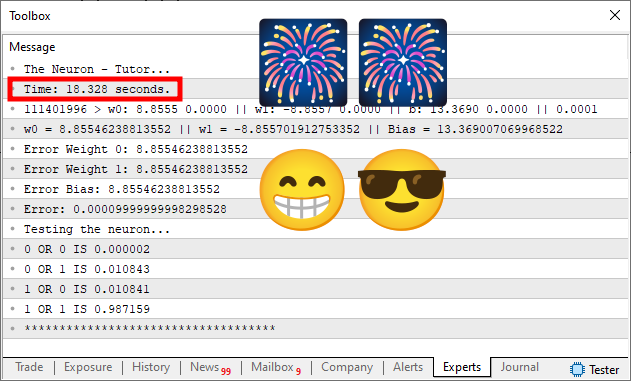
"What? But how is that possible? How did the time drop from almost 80 seconds to just over 18 seconds? That is absolutely impossible. Ah, I know, you changed computers and used another, more powerful one for this. Or, almost certainly, you somehow cheated by introducing another error into the system or changing something else. That way, the first run takes longer, as shown in the first image, but then you would spend much less time by using some trick. That way, you would get the image that can be seen in the second figure."

Well, dear readers, perhaps we could have done that. But no, that is exactly why we left the code in the attachment. By trying the same code on your own computer, you will be able to understand what happened. But before doing that, let us first examine why the code that previously took almost 80 seconds now runs in just over 18 seconds. First of all, I will say that there is no magic or anything like that here. It is a matter of understanding what the neuron must learn.

If you look at the code, it may seem very complicated, especially if you are just starting to program. However, do not worry; it is quite simple. I made sure that it stayed that way. This makes the explanation of how it works more visual and practical.

Let us begin with line 07. It contains a definition, and this is one of the few places where you, as beginners, will have to modify the code without risking making it unstable. If line 07 is removed, the code will remain exactly the same as in the previous section. In other words, slow and inefficient, but still universal. However, if the macro on line 07 is defined as shown here in the article, the fast version of the code will be used, and you will see the result shown in the image above.

Now I want you to compare the image from this topic with the images from the previous one, while paying attention to the error value. Please note how similar they are. This is especially true of the last image from the previous topic and the one shown here. In other words, in both cases we use an error of 1e-4. "Wait a minute. Are you saying that despite using the same precision, the execution time dropped sharply?" Yes, dear readers, that is possible. That is exactly what happened. "But why did this happen? Could you explain it to me?"

All right, to understand this, we need to look at a few points in the code. Let us skip most of the code and move on to the OnStart procedure, which is located on line 50. Now we need a little patience, but understanding what is happening is not difficult at all. Please note that most of the code in this procedure has already been discussed in the previous section. These identical parts are what make the neuron the same as the one we saw before. However, it is on line 62 that we ask the compiler to perform a check before creating the final executable file. This test checks whether the definition on line 07 is present.

If it is not present, the resulting code will be identical to what was discussed in the previous topic. If the macro on line 07 is defined, the code from the previous topic will be replaced by the code located on line 63. Pay attention to this. We replace the code between lines 65 and 73 with the code from line 63. Everything else remains unchanged and untouched.

But now, looking at the contents of line 63, we can see that it is a for loop. It is very similar to the code in line 65. Of course, the difference is that in line 65 we call Cost, while in line 63 we call Cost_2. In all other respects, the code is identical. "But this does not explain why in one case it takes almost 80 seconds, while in the other it takes only 18 seconds. Such things make absolutely no sense." But this is exactly where you are mistaken, dear readers. This simple change can make all the difference. Please note that although we are looking only at line 65, the Cost function is actually called four times: in line 65, line 67, line 68, and line 69.

For each of these calls, the entire table, database, or, in our case, training array must be analyzed. Think about that for a moment. Notice that our training array contains only four rows of data. This can be seen in line 09 of the code. Only four rows of data. However, every time the Cost function located on line 19 needs to be called, the loop on line 24 will read and calculate everything again. This applies to all calls present in the OnStart procedure.

This programming style greatly simplifies the task, but it is generally not very efficient. However, this same programming style makes the neuron much more universal. This is because the neuron can be made to handle as many inputs or outputs as needed without requiring changes to that part of the code. This is exactly where knowing what we are doing, or knowing the expected or intended result, becomes crucial. Many would take this function from line 19 and convert it into OpenCL code, or even into code that could run on parallel systems. In some cases, machines that run parallel applications can be quite expensive.

In other cases, even a good graphics card will do. Nevertheless, we would simply be replacing one thing with another, because the code would still remain inefficient. We say this because every time the cost is calculated, we would have to scan the entire database used for training. Imagine a database containing thousands of megabytes of data.

Now let us return to line 63. At first glance, line 63 may not seem special, but it calls a specialized function. This greatly speeds up execution compared to non-specialized execution. However, having a specialized neuron makes programming somewhat more complicated, because if we need to change something in the neuron, whether the number of inputs or the number of outputs, we will have to completely change the code of the Cost_2 function, which is called less often on line 63. The reason lies precisely in its approach to operation. Let us see how this works and move on to line 30, where Cost_2 is implemented. But to make the explanation clearer, let us examine this function as a new topic.

Specializing a single neuron

Now, for those who want to study everything more calmly and essentially understand how it works, let us divide the Cost_2 function into two parts. This will make it easier to explain why it works faster than the standard version.

All right, the first part is between lines 35 and 41. What does the code in these lines do? It does the same thing that lines 65, 67, 68, and 69 used to do. In addition, of course, it also performs the same operation as the for loop in line 24. In other words, we ultimately execute line 25. However, unlike what was done before, we now do everything at the same time. As a result, we need more variables than before. Each of the variables declared in line 32 serves to speed up code execution. Thus, in line 37 we calculate the total error of the neuron. This will not speed up the process, but in lines 38, 39, and 40 we calculate all the other errors that were previously measured in the for loop located on line 65.

Now we come to the difficult part of the matter. Line 40 is part of every neuron. In other words, it is universal code, just like line 37. But lines 38 and 39 are not. They are precisely what specialize the neuron. In other words, if we need to add more inputs to the neuron, we will have to add more such lines to the code, and a neuron created for one purpose will most likely not be useful for anything else. However, this approach makes the code much faster than a more generic implementation optimized poorly for the task.

The second part of the code is on lines 43, 44, and 45. There we correct the values for the next call of the cost function. Previously, this was done on lines 70, 71, and 72.

Simply making these small changes to the code allowed the neuron to run much faster, enabling it to learn or, more precisely, produce a set of values that serves as stored prior knowledge. And that is the real beauty of this kind of programming. It is not about the call itself as a test, but about the pleasure of realizing that everything can be done much more efficiently. Please note that there was not even any need to use OpenCL or write parallelized code. This is far more engaging and enjoyable than all the dullness many people show, especially when the topic turns to neural networks.

All right, this was a fairly simple example of how this can be done, but we can go a little further on the same issue. Although this simple neuron is capable of many things, and its only limitation is the need to keep increasing or decreasing the number of inputs while, of course, always trying to do so as quickly as possible, it is still not "intelligent" enough to handle certain types of situations. Therefore, artificial intelligence or neural networks are not as simple as many people believe. Likewise, one cannot assume that a neuron will be able to handle any situation within a particular scenario.

To illustrate this, let us perform a small thought experiment. There is nothing complicated here; I simply want to show you something that many people overlook when studying neural networks. Many people remain silent about this or do not want to talk about it, but if you understand it, you will realize that no program can surpass the mind that created it.

Let us consider the data used for training. There are situations where a neuron cannot process the data. And it is not because the data is extremely complex or anything like that; in essence, the data is simple. But a single neuron does not solve the problem, and I repeat, it DOES NOT solve it, so more than one neuron must be used for this. Thus, we will briefly outline a topic that will be discussed later. However, in some specific cases, it is acceptable to model a small neural network using a single neuron. It all depends on the type of task for which we are looking for a solution.

Thus, in many cases, and in fact in most of them, a neuron can be built or, better said, programmed so that it can be used in the future to implement a neural network. And I am not talking about neural networks like chatbots or anything similar; I am talking about something much simpler. However, there are cases where we can make a single neuron solve a task that would normally require a small neural network. And we do not need to create BIG DATA with a huge amount of data to find a situation where this happens. This can be done using the same code shown in this article.

"Wow, now everything has really become much more complicated. Why? Let me see if I understood you correctly. Are you saying that this neuron we are working with cannot handle something that can be represented in this same database, but if we know how to deal with it, we can make it imitate a small neural network and thus solve a task that it cannot solve on its own? Is that right?" Yes, that is correct. Please note that the training dataset we are using resembles a logic-gate truth table. In other words, we can feed it combinations of zeros and ones and ask the neuron to try to find an equation or, more precisely, a linear function that could represent a logical gate.

Nevertheless, there are two cases, although we can treat them as one. This is because they are inverses of each other. In these cases, this simple neuron will not be able to find the correct equation, but if we force it to work in a certain way, it will be possible to find the correct equation.

To make what I want to explain easier to understand, look at the following image.

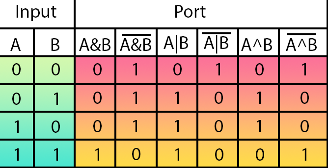
This image shows the main logical gates considered here. The green section contains the gate inputs. The outputs are shown in red and orange tones, and the gate type is indicated at the top of each diagram.

Now let us see what this means. From left to right, the gates are arranged in the following order: AND, NAND, OR, NOR, XOR and NXOR.

And what significance does this table in the image have for us if our topic is neural networks? To understand this, let us look at the neuron code once again. Notice that in line 09, where we define the training rules, we have something exactly like the table shown in the image.

Now comes the interesting part: the first two values are the input data. The third value, on the other hand, is the result. Compare what you see in the code with the table shown in the image. What do you notice? Well, if you look a little more closely, you will notice that in the training process we define the AND gate.

You can experiment by changing the values of the third argument used in training. You will see that you can make the neuron learn or generate an equation capable of representing almost all gates. I say "almost" because the neuron will not be able to learn two of them. These gates are precisely XOR and its inverse, NXOR.

"Wow! But wait a minute. Why will the neuron not be able to learn to generate the XOR and NXOR gates? Are you joking? All the values consist exclusively of zeros and ones. This can only be a joke or a prank. Are you making fun of me?"

I would even like to joke and tease you, but in fact that is not the case. This is a fact, and you can verify it. If you try to train a single neuron using only zeros and ones, then in some cases the neuron will not be able to learn how to handle the situation. This is because the solution is much more complex than what can be modeled with a single neuron.

You are unlikely ever to hear someone talk about such things or even mention them. This happens when the topic we are studying is somehow related to artificial intelligence, neural networks, or neuron programming. People do not think about trying all the alternative options. If something works in a particular case, they immediately start spreading the word about it. But if you ask them about specific situations, they start beating around the bush or ignoring the question.

However, there is a way to train a neuron to deal with such cases, for example when we need to solve the XOR gate problem or its inverse, the NXOR gate. Since this topic is quite difficult to explain within the scope of this article, in the next publication we will examine how to solve this issue. But before the next article is published, perhaps you, my dear readers, can come up with a way to solve the problem of the XOR gate and its inverse, the NXOR gate, on your own. Note: you cannot use more than one neuron; that would be cheating. The rule is this: only one neuron may be used to implement the solution.

Final thoughts

In this article, we showed how a small change in the code aimed at specializing the neuron can make the training phase significantly faster. Since once a neuron or neural network, as we will see later, has been trained, the work it performs becomes much faster. So much so that in the code presented both in the article itself and in the attachment, you can see that generating results from input data happens very quickly. Of course, this is provided that we already know which values should be used in the calculation.

Here we also mentioned an existing problem that almost no one talks about or even mentions. It is precisely that a neuron is not capable of handling all possible scenarios, contrary to what many people are used to believing. A machine is not so perfect and is not capable of surpassing a living being. A single biological neuron is capable of solving any simple task. Nevertheless, a programmed neuron or one implemented in silicon is not capable of such a feat.

So, in the next article, we will continue examining this issue. See you later, and see you soon.