Neural Networks in Practice: Gradient Descent

Introduction

In the previous article, “Neural Networks in Practice: An Example of Implementing an XOR Gate”, we examined how this problem can be solved—or, more precisely, the fact that a single neuron is incapable of learning to represent an XOR gate or its inverse, NXOR. Although a single neuron is capable of describing various cases, I think it has become quite clear by now that there are situations it cannot handle, even if they seem fairly simple at first glance.

And although at first glance it might seem that a neuron is capable of representing this same data, there are situations where this simply does not happen. That has been the goal all along: to show that, contrary to what many people say or would have you believe, there are cases where we cannot get a solution to work simply because it works in a simple, specific case.

Thus, an artificial neuron is by no means as unusual as many people think. In and of itself, it's just a simple mathematical calculation. And that's all there is to it. Nevertheless, I think you've already noticed that, although we can make an artificial neuron represent something, in some cases we may run into certain difficulties. This is because every time a change is needed, we’ll have to modify the neuron in some way so that it behaves as it should and can represent certain types of data. In many cases, this kind of situation makes the project completely unviable.

As those of you who have been following these articles on neural networks have probably already noticed, there is no definitive solution. There are solutions that cover a greater or lesser number of cases, but none of them is definitive. That doesn't prevent us from choosing a specific direction or trying to develop something that will make the use of artificial neurons practical.

When studying neural networks—especially at the very beginning—many questions arise that can be confusing to varying degrees. I know this because I went through the same process myself when I started learning to program in C/C++. At that time, this topic wasn't as prominent or as widely discussed. To tell the truth, few people spoke about this, and those who did were quite skeptical.

Unlike the current situation, in which the media as a whole seems to be overhyping the topic and making all kinds of claims about neural networks. And, what's worse, many people—especially investors—were saying things that were far from reality. I'm not here to judge anyone or stir up controversy. I just want to share what I know in as accessible a way as possible. That way, at least, you'll have a starting point to gain a better understanding of this topic.

Well, in this article, we're going to do something a little out of the ordinary. I know that many people think my articles on neural networks form a series, although in reality it's impossible to create a series of articles on this topic. Believe me: as strange as it may sound, it's practically impossible to write a series of articles about neural networks. This is because we have to return to the basics time and time again. And the reason is simple: HUMANITY HAS NO CLEAR IDEA OF HOW TO DEVELOP SOMETHING LIKE THIS.

What I just said may seem completely illogical, since, apparently, something new on this topic comes up every day. In practice, however, things aren't quite like that. In reality, what happens is this: we have to go back to what we’ve already done, time and time again, and rethink it as we try to solve some new problem that has arisen.

In previous articles, you've probably noticed that, even though everything works, we're still facing a number of problems. All of these problems have already been solved or are being solved right now, one way or another. Among the issues I can mention here—and which we have already discussed in these articles—the following stands out: the more variables or parameters we have to process, the slower the neuron or neural network becomes. In addition, as we have to process more and more variables, computational resource consumption also increases. Another problem is that we have little flexibility when it comes to changing the number of parameters or variables in a neuron.

This problem can be better understood as follows: let's start with a single input to a neuron. This was discussed in the early articles, which presented the first diagram of a neuron. But soon we had to add a new input. So, the previous code looked roughly as shown in the following snippet:

//+------------------------------------------------------------------+
double Cost(const double w)
{
    double err;

    err = 0;
    for (uint c = 0; c < nTrain; c++)
        err += MathPow((Train[c][0] * w) - Train[c][1], 2);

    return err / nTrain;
}
//+------------------------------------------------------------------+

Before long, it looked as shown in the following snippet:

//+------------------------------------------------------------------+
double Cost(const double w0, const double w1, const double b, const double &Train[][])
{
    double err;

    err = 0;
    for (uint c = 0; c < nTrain; c++)
        err += MathPow(((Train[c][0] * w0) + (Train[c][1] * w1) + b) - Train[c][2], 2);

    return err / nTrain;
}
//+------------------------------------------------------------------+

Notice that the code began to grow and become somewhat more complex. But if you don't believe that, I want you to think about this: every time a new variable or parameter is added to a neuron, we'll have to change the code. Since each new parameter represents a new input, if at some point we need to use a thousand inputs, we'll have to include all thousand of those variables in the code. And all of it by hand. Just think about the enormous amount of manual work that would require.

Another issue has to do with how we perform the calculations to adjust the variables. In other words, how a neuron or a neural network will represent a specific dataset. Perhaps this question carries the most weight when deciding which neuron implementation to choose. To make things clearer, let's use the code we looked at in the previous article as a starting point. This code is shown in the following snippet.

//+------------------------------------------------------------------+
double Cost(const double w0, const double w1, const double b)
{
    double err;

    err = 0;
    for (uint c = 0; c < nTrain; c++)
        err += MathPow((macroSigmoid((Train[c][0] * w0) + (Train[c][1] * w1) + b) - Train[c][2]), 2);

    return err / nTrain;
}
//+------------------------------------------------------------------+
double Cost_2(double &w0, double &w1, double &b)
{
    double err, ew0, ew1, eb;

    err = ew0 = ew1 = eb = 0;
    for (uint c = 0; c < nTrain; c++)
    {
        err += MathPow((macroSigmoid((Train[c][0] * w0) + (Train[c][1] * w1) + b) - Train[c][2]), 2);
        ew0 += MathPow((macroSigmoid((Train[c][0] * (w0 + eps)) + (Train[c][1] * w1) + b) - Train[c][2]), 2);
        ew1 += MathPow((macroSigmoid((Train[c][0] * w0) + (Train[c][1] * (w1 + eps)) + b) - Train[c][2]), 2);
        eb += MathPow((macroSigmoid((Train[c][0] * w0) + (Train[c][1] * w1) + (b + eps)) - Train[c][2]), 2);
    }

    w0 -= (((ew0 - err)/ eps) * eps);
    w1 -= (((ew1 - err)/ eps) * eps);
    b  -= (((eb - err)/ eps) * eps);

    return err / nTrain;
}
//+------------------------------------------------------------------+

In it, we adapted the code to make it run faster. This brings us to the first problem: computational cost increases as the number of tasks we need to perform grows. Or, as many people say: the more things we need to analyze, the more computing resources we'll need. Although both functions in the previous code snippet use exactly the same calculations, their execution speeds vary greatly. This is precisely because the first function has to be called repeatedly. The second one, however, is called much less frequently, and that makes all the difference.

In addition, there is one more question. You may not have noticed, but from the very beginning, all the code has been centered around a single mathematical formula. This formula is the linear regression formula. Yes, we used different methods to obtain linear regression. But in the end, they all came down to using linear regression.

If linear regression works, why try a different method? So, this brings us to another issue related to neural networks. The goal of every method is to create a mathematical representation of the data we use. If you use a faster method, you'll need fewer computing resources to achieve the same results.

In the worst-case scenario, we can resort to a brute-force search, which, although it works, is completely impractical. This is because a brute-force search always requires far more computational resources than a method based on a mathematical formula. Linear regression works in many cases. However, as the number of parameters increases, it, too, begins to face the same problem as a brute-force search. In other words, completing it within a reasonable timeframe requires more and more computing resources.

If you look at the linear regression formula we're using, you'll notice something curious and interesting. And that is exactly what we will focus on in this article. Let's now move on to a new topic to understand what we'll be doing next.

Derivatives again, but under a new name

To make things as simple as possible, let's go back to the most basic concepts so you can follow the mathematical reasoning we'll be using. I don't really like to include formulas and things like that, because they often make it seem as if everything is much more complicated than it actually is. But there's no other choice. To explain this properly, we need to turn to mathematics for a moment. In most cases, linear regression is calculated using the least squares method. In other words, you take the error resulting from the calculation and square it. Add up all the squares you've obtained—and you'll get the total error. This is exactly what the following equation expresses.

Here, I'm breaking it down to the most basic level. Therefore, the bias is not taken into account here. Only the weight is used. So, the value < k > reflects the total number of data points we use. Or, more precisely, it shows how much data we have for performing a linear regression. The value < x > corresponds to the data used during training, as does the value < y >. The difference is that x represents the input data, and y represents the expected result. The only thing we need to change is the weight, which corresponds to the value < w >. All right, those are the basics.

This equation tells us the following: if we substitute an arbitrary value for < w >—which is the only thing we can change—we will obtain an equally arbitrary error. If we then arbitrarily change the value of < w > again, we will get a new error. By comparing these two errors, we'll be able to tell whether we're heading in the right direction or the wrong one. If we're heading in the right direction, we can keep going; if we're heading in the wrong direction, we need to stop and change course. That is all that is required. In the same equation given above, there is one detail that catches our attention: we are squaring the value. And this fact alone allows us to find its derivative. This is where the analysis really starts to get interesting.

When this equation is differentiated, it is given a new name. This can be explained by a rather interesting feature of the equation itself. New name: GRADIENT DESCENT. You've probably already heard of gradient descent. But do you know where that came from? Well, if the answer is “no,” then now you know. Gradient descent is an equation obtained by differentiating linear regression. I won't show how to convert linear regression into gradient descent here, as that is completely beyond the scope of this article.

If you're interested in learning how this is done, I'll provide a source in the links section at the end of the article where you can explore this topic. That said, be prepared to deal with quite a bit of math. The explanation provided there is much better than any I could give here, since our focus is on programming itself. When you differentiate—that is, when you transform the previous equation—you will obtain the following equation.

This is true only when the weight is the only factor taken into account. But what if we also want to use a bias? In that case, we'll have two different functions, not just one, as you might have expected. These two functions are listed below.

Here, we seek the minimum of the cost function by varying only the weight, based solely on the weight. In other words, we vary the weight while keeping the bias constant, aiming to find the minimum cost with respect to the weight. In the following figure, on the other hand, we attempt to reduce the loss function by adjusting the bias. In other words, we keep the weight constant and change only the bias.

"Oh, wait a minute. Is the only difference between them at the end of the equation?" Yes, my dear reader. To help you understand this and the reason for this difference, I suggest you review the materials I’ve provided for reference, or study on your own how the derivative is calculated in this case. This will help you gain a deeper understanding of the mathematical concepts related to this gradient descent method.

Although gradient descent is just one of many methods for minimizing the loss function to fit a straight line—or, more generally, an equation that represents the data, I must admit that it is currently one of the most widely used. Nevertheless, there are methods that, in some cases, prove to be more effective. In other cases, even the gradient descent method itself may undergo further mathematical transformations in order to develop an even more sophisticated methodology.

This is precisely why you encounter so many mathematical terms when studying neural networks. It's not that one methodology is better or worse than another. The fact is that we programmers are always looking for new ways to perform computations, but we're all pursuing the same goal: to reduce computational cost. In other words, do the same thing, but faster. This is precisely the goal of all this research in mathematics when it comes to neural networks.

Okay, so how do we implement all of this in code? That's exactly what we're really interested in, and that's exactly why I wrote this article. To see this, let's move on to a new topic.

Programming a Neuron Using Gradient Descent

Here, we'll go back to the simplest code of all. In other words, we won't be dealing with activation functions, bias, multiple inputs, and the like. Let's start again with the original system: one input and one output, as if we hadn't done anything before. That way, you'll be able to truly understand how to implement it. If we had started with something more complicated, you would have spent a lot of time trying to figure out why it works—or why it doesn't work the way you expected. So, let's start from scratch again.

To do this, let's take a look at the first neuron we discussed in these articles on neural networks. The complete code is shown below.

01. //+------------------------------------------------------------------+
02. #property copyright "Daniel Jose"
03. //+------------------------------------------------------------------+
04. #define PrintEx(A) Print(#A, " => ", A)
05. #define macroRandom (rand() / (double)SHORT_MAX)
06. //+------------------------------------------------------------------+
07. double Train[][2] {
08.                     {0, 0},
09.                     {1, 3},
10.                     {2, 6},
11.                     {3, 9},
12.                     {4, 12},
13.                   };
14. //+------------------------------------------------------------------+
15. const uint nTrain = Train.Size() / 2;
16. const double epsilon = 1e-3;
17. //+------------------------------------------------------------------+
18. double Cost(const double w)
19. {
20.     double err, factor;
21. 
22.     err = 0;
23.     for (uint c = 0; c < nTrain; c++)
24.     {
25.         factor = Train[c][0] * w;
26.         err += MathPow(factor - Train[c][1], 2);
27.     }
28. 
29.     return err;
30. }
31. //+------------------------------------------------------------------+
32. void OnStart()
33. {
34.     double weight, err, e1;
35.     ulong it0, it1, count;
36. 
37.     Print("************************************");
38.     Print("Linear regression neuron...");
39.     MathSrand(512);
40.     weight = (double)macroRandom;
41. 
42.     it0 = GetTickCount();
43.     for(count = 0; (count < ULONG_MAX) && ((err = Cost(weight)) > epsilon); count++)
44.     {
45.         e1 = (Cost(weight + epsilon) - err) / epsilon;
46.         weight -= (e1 * epsilon);
47.     }
48.     it1 = GetTickCount();
49.     Print("Time: ", (it1 - it0) / 1000.0, " seconds.");
50.     PrintEx(count);
51.     PrintEx(weight);
52.     PrintEx(err);
53. }
54. //+------------------------------------------------------------------+

Of course, I made some changes to the code to make it even simpler and more intuitive, so that even those who aren't very familiar with math but have a basic understanding of programming can easily understand it. It doesn't take anything special; you don't have to be a programming Jedi master to understand what's going on. In addition, code very similar to this one has already been explained. The idea and the way it works, however, remain the same. Please note that on line 38, I specify which model was used for the loss function. When you run this code in the MetaTrader 5 terminal, you will see the following image:

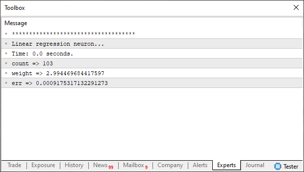
Take a look at the data in this image, because I want you to compare it with what we'll see in the following code. All right, now we have a benchmark. Now let's consider this same neuron—or, more precisely, this same training process—but using a loss function based on gradient descent. The complete code is shown below.

01. //+------------------------------------------------------------------+
02. #property copyright "Daniel Jose"
03. //+------------------------------------------------------------------+
04. #define PrintEx(A) Print(#A, " => ", A)
05. #define macroRandom (rand() / (double)SHORT_MAX)
06. //+------------------------------------------------------------------+
07. double Train[][2] {
08.                     {0, 0},
09.                     {1, 3},
10.                     {2, 6},
11.                     {3, 9},
12.                     {4, 12},
13.                   };
14. //+------------------------------------------------------------------+
15. const uint nTrain = Train.Size() / 2;
16. const double epsilon = 1e-3;
17. //+------------------------------------------------------------------+
18. double Cost(const double w)
19. {
20.     double err, x, y;
21. 
22.     err = 0;
23.     for (uint c = 0; c < nTrain; c++)
24.     {
25.         x = Train[c][0];
26.         y = Train[c][1];
27.         err += 2 *(x * w - y) * x;
28.     }
29. 
30.     return err;
31. }
32. //+------------------------------------------------------------------+
33. void OnStart()
34. {
35.     double weight, err;
36.     ulong it0, it1, count;
37. 
38.     Print("************************************");
39.     Print("Linear gradient neuron...");
40.     MathSrand(512);
41.     weight = (double)macroRandom;
42. 
43.     it0 = GetTickCount();
44.     for(count = 0; (count < ULONG_MAX) && (MathAbs(err = Cost(weight)) > epsilon); count++)
45.         weight -= (err * epsilon);
46.     it1 = GetTickCount();
47.     Print("Time: ", (it1 - it0) / 1000.0, " seconds.");
48.     PrintEx(count);
49.     PrintEx(weight);
50.     PrintEx(err);
51. }
52. //+------------------------------------------------------------------+

When you run this code in the MetaTrader 5 terminal, you will see the following image:

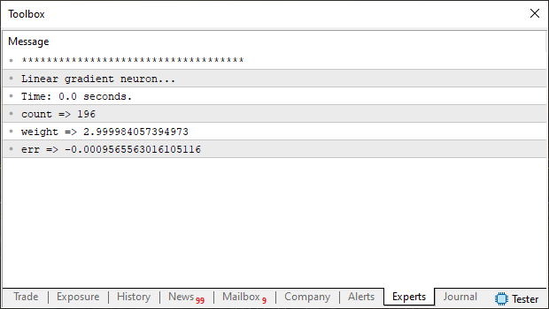
Now compare the two images: the one obtained using gradient descent and the one obtained using linear regression. Have you noticed any difference? Is your answer "yes," "no," or "maybe"? Well, so you don't have to strain yourself trying to spot the difference, the next image shows both results together. That way, it will be easier to notice the difference.

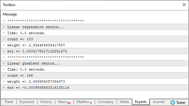
Well, I don't notice any difference, except maybe in the counter. Well, my dear reader, if this applies to you, take another look—without rushing. Note that linear regression appears to have worked faster. However, the weight value it obtained is slightly less accurate than the value obtained using gradient descent. You might be thinking right now, “Okay, but we need the loss function to run as quickly as possible, don’t we?” Yes, my dear reader, and I completely agree with that point. That's exactly why I'm showing this comparison.

I want you to avoid falling for the misconception held by those who claim or stubbornly insist that gradient descent is better than linear regression. It all depends on the circumstances. And this depends primarily on the type of data we use to train the neuron. That is, it depends on the type of data we use to obtain the parameters of the equation. These values are intended to reflect the data from our dataset as accurately as possible. The method that is considered the best does not always actually turn out to be the best. Every case is unique.

Please also note that the error value is different. In the case of linear regression, it will always be positive. In the case of gradient descent, on the other hand, it can sometimes be positive and sometimes negative. This is because the function itself tries to find the best point for reducing the loss function. "But wait a minute. How so? I don't understand that. Shouldn't the result always be the same, regardless of the type of function we use to find the best representation of the data?" No, my dear reader, and this is yet another of the mistakes or misconceptions that many people repeat when it comes to neural networks. Or, more precisely, when it comes to training a neural network, whether it uses one neuron or several. To explain this, let's move on to a new topic. That way, I'll be able to better distinguish between these concepts.

What exactly is this “loss function” that is so often mentioned?

The quantity that everyone refers to as “loss” is the error of the function—or, more precisely, of the representation generated by the function—relative to the actual data contained in the dataset and used to construct that function. Okay, but what's the problem here? I just can't understand why a dataset containing the exact same data can generate such different functions. Shouldn't they be the same, regardless of the type of modeling used to construct a representation of the data from the dataset? There's definitely no easy answer to this question. In any case, it will depend on the specific situation.

All the examples I've given are designed to be as simple as possible. Therefore, in all cases, the overall function describing the training data can easily be represented as a parabola. In other words, we have a single point of convergence for the system. Thus, regardless of the starting point, the models will always converge to this single point. However, in REAL-WORLD conditions, this isn't always the case. The curve that best fits the data from the dataset can be a fairly complex polynomial. It can be of the third degree or higher, and the higher the degree, the greater the influence of the starting point when searching for the best representation of the data. In other words, even if the modeling method we use cannot converge to the point where the loss function is minimized, we will still get the impression that we have found the best possible point.

It's much harder to illustrate situations like these than it seems. Nevertheless, they happen more often than you, my dear reader, might imagine. To illustrate what I just said a little better, let's imagine the following: suppose you have a dataset whose entire contents can be represented by a mathematical function. And when you plot this function, you get the graph shown in the following image:

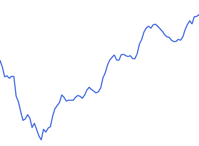
My question is this: which neural network is best suited to constructing a mathematical representation of this dataset? The idea is to avoid losing any data because the graph of the representation generated by the neural network differs from the one shown above. Hmm, now we really have a problem, don't we? And it is precisely this area that is the focus of all research in the field of neural networks. Everything—absolutely everything—boils down to this.

You might think: we could use linear regression. Or perhaps gradient descent. Or stochastic gradient descent. Or we can use a brute-force search. Yes, my dear reader. In the worst-case scenario, it could all come down to brute-force search. But consider the computing power required to construct an equation that represents this data. These days, that's practically unthinkable. Perhaps a quantum computer will actually be developed someday. But until then, let's forget about brute-force search. We need to use a different method. And that's exactly where the problem arises.

It is clear that there is a minimum point on this curve. It is precisely at this point that the function will have the smallest possible loss—at least, judging by the graph. However, many argue that, in trying to find this point, we will actually be overfitting. But that's complete nonsense. The idea here is to create a function that, ideally, would represent all the data contained in the dataset. So where did this idea of overfitting come from? The thing is, this idea arises because everyone wants to find the best function, but once we find it, we might simply fail to recognize elements that are outside the dataset.

In addition, there is another reason: computational cost. Think about this. Any modeling method designed to represent a dataset requires one or more inputs. Once these initial values have been processed, the function’s initial loss is calculated. And here's the key point. Where is this starting point? So, let's go back to our drawing and this time add a few points to the line.

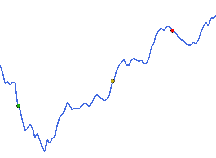
Each of these points was generated completely at random, just as we always initialize a neuron or a neural network. However, they reflect the initial loss resulting from these random initial values. And now comes the most interesting part. Which of these points will actually reach the point with the least loss on this curve, shown in blue? Well, that will depend on how each point searches for the point with the least loss. Depending on how each of them performs the search, it may turn out that none of them ever reaches the point of convergence with the lowest loss. This is because their path is marked by both valleys and peaks, and no one knows for sure how to overcome those peaks. They are always looking for the deepest valley, starting from the peak at which they began. Therefore, the issue of overfitting is not really the main problem. The real problem is this: how many computational resources will be wasted searching for the deepest valley or the point with the lowest loss?

Concluding Thoughts

In this article, I have tried to explain as simply and clearly as possible one of the most controversial issues that arises when discussing neural networks: how to find the best possible point or the minimum of the loss function. I demonstrated the difference between linear regression and gradient descent. Both methods are fairly simple and serve as examples of how the path that seems obvious isn't always the best one.

There is still much work to be done in the field of neural network research. So, if you're interested in this, try to take your time when studying the topic and always look for high-quality resources. There are many uninformed people who simply repeat misconceptions that they themselves don't even understand. The code used in this article is provided in the attachment.

Despite everything that has been said here, we will return to this topic later. Here, I have only briefly touched on what really lies at the heart of this issue.

Link

Linear Regression and Gradient Descent: From Zero to Magic