Neural Networks in Practice: When to Use an Artificial Neuron and How It Works in MQL5

Introduction

In the previous article “Neural Networks in Practice: Stochastic Gradient Descent”, we made some changes to create a small neuron that uses gradient descent. We made these changes to make it easier to explain certain aspects of how a neuron works. The main goal was to clarify a concept that causes a lot of confusion and is often discussed without a true understanding of its essence. Now we'll begin to understand why activation functions are necessary in some cases but not in others. We'll also see why a neural network isn't always the best choice. But above all, we'll understand why there are different neural network architectures and how to properly determine the size and configuration of a neural network. And, of course, we'll cover other topics in the following articles.

I realize that this introduction may seem quite interesting and, at the same time, somewhat ambitious for a single article. It would be impractical to explain all of that in a single article, as it would end up being too long. Let's take a closer look at why, after we've already covered so much, I'm only now saying that we'll begin to analyze these details related to neural networks. The reason is simple: I first had to explain a whole series of concepts so that you, my dear reader, could finally understand what this is really about.

Essentially, I'd say that this is Article Zero—the starting point from which we'll really begin to have a serious discussion on this topic. This is because, by now, if you’ve read the previous articles, tried out the code provided in them, attempted to modify the training set, or compared the earlier articles with the more recent ones, you’ve likely already grasped the logic behind what I’m about to explain.

If you went straight to this article, aren't familiar with neural networks, and have a lot of questions on this topic, I recommend that you first read the previous articles to understand what will be explained later on. All right, let's get started.

Do I really need to build a neuron?

Judging by what the media, influencers, and others have been saying for some time now, it seems that we can’t do without neural networks. As if they were the eighth wonder of the modern world. Actually, that's not quite how it is. As you've probably noticed from previous articles, the study of neural networks is a rather interesting field of research. However, in general, they have limitations and can malfunction. They cannot handle certain types of tasks and aren't as versatile as many people claim.

In many cases, a program designed to solve a specific problem will be significantly more effective than any neural network we could build. This is due to a number of factors. If you, my dear reader, decide to use a neural network for a particular task, you'll have to train it so that it can perform that task. In addition, it may be the case that it won't even be able to interpret the data you're using to train it.

I haven't mentioned this yet. Although it isn't always necessary, in most cases you'll need to normalize the values that the neural network will use. We'll get into why later, but it's something you should keep in mind. Sometimes you'll need to normalize the input values or scale them to a specific range. If this is not done, the neural network will not be able to converge and form an adequate representation of the training data.

Even if you manage to get a neural network to work, you'll have to take another factor into account: computational cost. It's not easy to explain this issue, since there are several factors at play here that I haven't yet discussed in these articles. Nevertheless, based on what we’ve already discussed, there are several factors that will help you, my dear reader, understand why a neural network isn’t always the best choice.

To see this for ourselves, let's run the following test. Let's take the neuron from the previous article and feed it some of the data we used at the beginning of this series. The new neuron code will look like this:

001. //+------------------------------------------------------------------+
002. #property copyright "Daniel Jose"
003. //+------------------------------------------------------------------+
004. #include <Canvas\Canvas.mqh>
005. //+------------------------------------------------------------------+
006. #define PrintEx(A)  Print(#A, " => ", A)
007. #define macroRandom (rand() / (double)SHORT_MAX)
008. #define _SizeLine   300
009. #define nColuns     2
010. //+------------------------------------------------------------------+
011. CCanvas canvas;
012. //+------------------------------------------------------------------+
013. double Train[][nColuns] {
014.                             {-100, -150},
015.                             { -80,  -50},
016.                             {  30,   80},
017.                             { 100,  120},
018.                   };
019. //+------------------------------------------------------------------+
020. const double epsilon = 1e-3;
021. //+------------------------------------------------------------------+
022. struct stErr
023. {
024.     double  Weight,
025.             Bias;
026. };
027. //+------------------------------------------------------------------+
028. stErr Cost(const double w, const double b, const uint p1 = 0, const uint p2 = Train.Size() / nColuns)
029. {
030.     double x, y, t;
031.     stErr err;
032. 
033.     ZeroMemory(err);
034.     for (uint c = p1; c < p2; c++)
035.     {
036.         x = Train[c][0];
037.         y = Train[c][1];
038.         t = 2 * ((x * w + b) - y);
039.         err.Weight += (t * x);
040.         err.Bias += t;
041.     }
042. 
043.     return err;
044. }
045. //+------------------------------------------------------------------+
046. void PlotText(const int x, const int y, const uchar line, const string sz0)
047. {
048.     uint w, h;
049. 
050.     TextGetSize(sz0, w, h);
051.     canvas.TextOut(x - (w / 2), y + _SizeLine + (line * h) + 5, sz0, ColorToARGB(clrBlack));   
052. }
053. //+------------------------------------------------------------------+
054. inline double CallZoom(void)
055. {
056.     double d1 = 0;
057. 
058.     for (uint c = 0; c < Train.Size() / nColuns; c++)
059.     {
060.         d1 = MathMax(d1, MathAbs(Train[c][0]));
061.         d1 = MathMax(d1, MathAbs(Train[c][1]));
062.     }
063. 
064.     return _SizeLine / d1;
065. }
066. //+------------------------------------------------------------------+
067. void Plot_Train2D(const int x, const int y, const double weight, double bias)
068. {
069.     int vx, vy;
070.     double zoom;
071.     uint n = Train.Size() / nColuns;
072. 
073.     zoom = CallZoom();
074.     canvas.LineVertical(x, y - _SizeLine, y + _SizeLine, ColorToARGB(clrRoyalBlue, 255));
075.     canvas.LineHorizontal(x - _SizeLine, x + _SizeLine, y, ColorToARGB(clrRoyalBlue, 255));
076.     for (uint c = 0; c < n; c++)
077.     {
078.         vx = (int)(Train[c][0] * zoom);
079.         vy = (int)(Train[c][1] * zoom);
080.        canvas.FillCircle(x + vx, y - vy, 5, ColorToARGB(clrRed, 255));
081.     }
082.     canvas.LineAA(
083.                 x + (int)(Train[0][0] * zoom), 
084.                 y - (int)((Train[0][0] * weight + bias) * zoom), 
085.                 x + (int)(Train[n - 1][0] * zoom), 
086.                 y - (int)((Train[n - 1][0] * weight + bias) * zoom), 
087.                 ColorToARGB(clrForestGreen));
088.     PlotText(x, y, 1, StringFormat("Zoom: %.2fx", zoom));
089.     PlotText(x, y, 2, StringFormat("f(x) = %.4fx %c %.4f", weight, (bias < 0 ? '-' : '+'), MathAbs(bias)));
090. }
091. //+------------------------------------------------------------------+
092. void OnStart()
093. {
094.     double weight, bias;
095.     int    x, y;
096.     ulong  it0, it1, count;
097.     stErr  err;
098. 
099.     Print("************************************");
100.     Print("Stochastic Gradient Descent Neuron...");
101.     Print("************************************");
102.     MathSrand(512);
103.     weight = (double)macroRandom;
104.     bias = (double)macroRandom;
105. 
106.     it0 = GetTickCount();
107.     for(count = 0; count < 5; count++)
108.     {
109.         err = Cost(weight, bias);
110.         if ((MathAbs(err.Weight) <= epsilon) && (MathAbs(err.Bias) <= epsilon))
111.             break;
112.         weight -= (err.Weight * epsilon);
113.         bias -= (err.Bias * epsilon);
114.         PrintFormat("%I64u > w0: %.4f %.4f || b: %.4f %.4f", count, weight, err.Weight, bias, err.Bias);
115.     }
116.     it1 = GetTickCount();
117.     Print("Time: ", (it1 - it0) / 1000.0, " seconds.");
118.     PrintEx(count);
119.     PrintEx(weight);
120.     PrintEx(bias);
121.     PrintEx(err.Weight);
122.     PrintEx(err.Bias);
123.     Print("Press ESC to close....");
124.     Print("************************************");
125. 
126.    x = (int)ChartGetInteger(0, CHART_WIDTH_IN_PIXELS, 0);
127.    y = (int)ChartGetInteger(0, CHART_HEIGHT_IN_PIXELS, 0);
128.    canvas.CreateBitmapLabel("BL", 0, 0, x, y, COLOR_FORMAT_ARGB_NORMALIZE);
129.    canvas.Erase(ColorToARGB(clrWhite, 255));
130.     x /= 2;
131.     y /= 2;
132.            
133.     Plot_Train2D(x, y, weight, bias);
134. 
135.    canvas.Update(true);
136. 
137.     while(!IsStopped())
138.         if (TerminalInfoInteger(TERMINAL_KEYSTATE_ESCAPE) !=0)
139.             break;
140. 
141.     canvas.Destroy();
142. }
143. //+------------------------------------------------------------------+

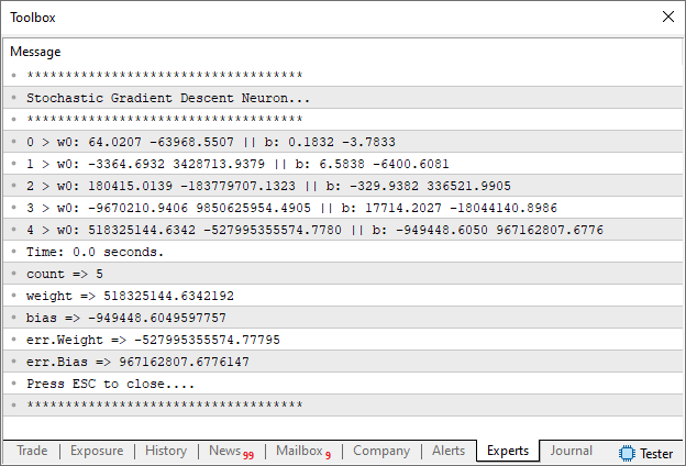
After compiling and running this code, you'll see the following in the terminal:

On the chart where you run the script, you'll see an image like this:

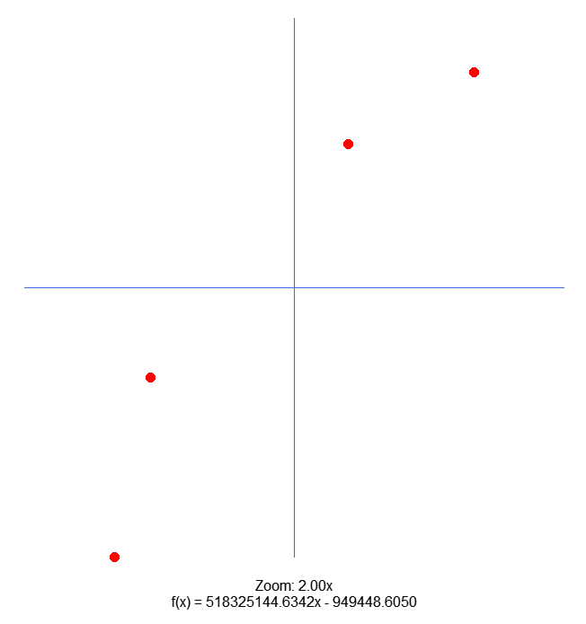
Well, perhaps you're now wondering, "What happened here? I don't understand a thing." Well, my dear reader, you don't understand what happened, and the artificial neuron can't interpret the data either: the neuron failed to converge to a solution. You might be thinking, "Wait a minute, you're cheating. There must be some kind of catch. How come the neuron couldn't interpret the training data?" And you're right to question that. We shouldn't believe something just because someone showed it to us or told us about it. We need to check this for ourselves to make sure it's true, although we should always exercise caution. So, let's take a look at what happened to produce the results shown in the previous images.

First, let's take a look at the code. Note that I changed the training data on line 13. I'll come back to this later. Let's now move on to the next change: on line 107, we reduced the number of iterations of the for loop from ULONG_MAX to five. That was a smart decision, as was adding line 114 to check what the neuron is doing internally. And, no matter how much some people may claim otherwise, NO, YOU SHOULD NEVER LET CODE GENERATE RESULTS WITHOUT UNDERSTANDING EXACTLY WHAT IT IS GENERATING. A while back, I heard someone say that soon we won't even understand what the network is learning. That's the biggest load of nonsense I've ever heard. There's no doubt about it—this person isn't a programmer; he just types in code.

But let's get back to the topic. We limited the loop to just five iterations to see if the neuron would begin to converge to a solution. If you look at the results, it becomes clear that this won't happen. In fact, the error values grow exponentially, which indicates that the neuron does not understand what it is doing or what it should do with the data. Remember that these were the only changes made to the code. You can take the code attached to the previous article and try it out. You'll see that the original version finds a solution, but once these changes are made, the neuron is more confused than a cockroach after being swatted with a slipper. Why did this happen? Doesn't this data make sense? Let's take a look at where this training data came from.

If you refer to the article “Neural Networks in Practice: Least Squares”, you’ll see that it uses precisely this data. There, as in other articles where we did not use neurons, we were able to find a solution. But here, the neuron can't handle it. Before explaining why, let's look at the equation obtained using other methods:

You don't have to take my word for it—you can check it out for yourself. In two articles, I demonstrated how to use the pseudoinverse matrix; the second of these is “Neural Network in Practice: Pseudoinverse (II)”. You can try it out for yourself and see that it works. So what's the problem here? Have we encountered the same problem as when using a neuron to represent logic gates? Or is this a case similar to the situation with the XOR gate? Neither is the case. To clarify this, let's move on to a new topic.

The Essence of an Artificial Neuron

Ever since we started breaking down the structure of a neuron, I've been showing how it works and why it does exactly what it does. If you still don't understand this, feel free to reread the previous articles, because here we'll delve into the topic in a bit more detail.

I'll repeat what I've already said: THE TRAINING OF ANY NEURON IS BASED ON A SECANT LINE. Many people like to talk about the tangent line when the topic of machine learning comes up. But, in my opinion, there are only two possibilities here: either they're confusing the concepts, or they don't know what they're talking about. The original neuron, from which all the others were derived, was built around the following function:

This function is, in fact, the loss function. Regardless of the method used, it all comes down to this function. However, it represents a secant line, not a tangent line. If we keep this in mind and recall that a straight line can be expressed by the following equation:

We can begin to understand why a neural network—or even a single neuron—is structured the way it is. Some people might think, “This guy doesn’t know what he’s talking about. Of course, the neuron couldn't interpret the training data: it lacks the activation function needed to learn how to represent them. Furthermore, it is not part of any network and does not use backpropagation.” Well, if that’s what you thought or if you’ve asked yourself that question, then—with all due respect—I suggest you stop reading this article and any of my other writings on this topic. None of them will be of any use to you if you've already formed a preconceived opinion on the matter. See you soon, and all the best.

Well, let's continue. The goal of any neuron is to find a secant for which h is as close to zero as possible. This value of h is the error we consider acceptable. In my programs, this same error value is also used as the learning rate: it determines what proportion of the error the neuron will use to calculate the next step and attempt to reduce it. In a neuron that uses linear regression or a function derived from it, the slope of the line is the weight, and the y-intercept is the bias. If you're looking for an image of a neuron, you'll usually find something similar to the following illustration.

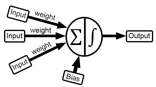
But what does this picture show? For some, it’s something magical; for others, it’s a summary of what needs to be implemented; and for still others, it’s absolutely nothing. Let's take a look at what we've implemented in our code. To do this, we need to modify the previous image so that we end up with the following.

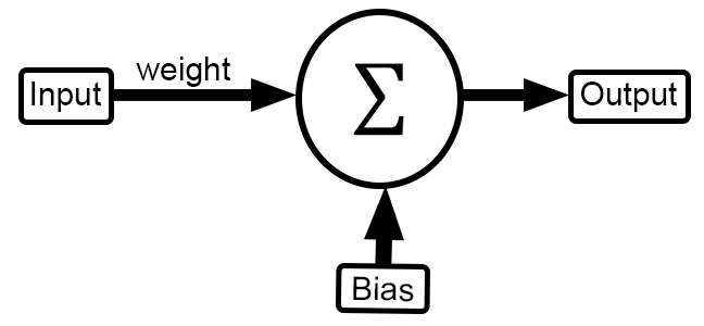
Well, yeah, it looks pretty similar to the previous image. But how can we tell if this resemblance is real, or if there's some kind of catch? To verify this, you need to examine the code—specifically, what happens in the following code snippet.

                                   .
                                   .
                                   .
012. //+------------------------------------------------------------------+
013. double Train[][nColuns] {
014.                             {-100, -150},
015.                             { -80,  -50},
016.                             {  30,   80},
017.                             { 100,  120},
018.                   };
019. //+------------------------------------------------------------------+
020. const double epsilon = 1e-3;
021. //+------------------------------------------------------------------+
022. struct stErr
023. {
024.     double  Weight,
025.             Bias;
026. };
027. //+------------------------------------------------------------------+
028. stErr Cost(const double w, const double b, const uint p1 = 0, const uint p2 = Train.Size() / nColuns)
029. {
030.     double x, y, t;
031.     stErr err;
032. 
033.     ZeroMemory(err);
034.     for (uint c = p1; c < p2; c++)
035.     {
036.         x = Train[c][0];
037.         y = Train[c][1];
038.         t = 2 * ((x * w + b) - y);
039.         err.Weight += (t * x);
040.         err.Bias += t;
041.     }
042. 
043.     return err;
044. }
045. //+------------------------------------------------------------------+
                                   .
                                   .
                                   .
091. //+------------------------------------------------------------------+
092. void OnStart()
093. {
094.     double weight, bias;
095.     int    x, y;
096.     ulong  it0, it1, count;
097.     stErr  err;
098. 
099.     Print("************************************");
100.     Print("Stochastic Gradient Descent Neuron...");
101.     Print("************************************");
102.     MathSrand(512);
103.     weight = (double)macroRandom;
104.     bias = (double)macroRandom;
105. 
106.     it0 = GetTickCount();
107.     for(count = 0; count < 5; count++)
108.     {
109.         err = Cost(weight, bias);
110.         if ((MathAbs(err.Weight) <= epsilon) && (MathAbs(err.Bias) <= epsilon))
111.             break;
112.         weight -= (err.Weight * epsilon);
113.         bias -= (err.Bias * epsilon);
114.         PrintFormat("%I64u > w0: %.4f %.4f || b: %.4f %.4f", count, weight, err.Weight, bias, err.Bias);
115.     }
116.     it1 = GetTickCount();

Indeed, our loss function may seem somewhat unusual, since it is actually the first derivative of the original function. Therefore, it does not resemble the equation of a straight line. However, if you look at the code, you'll see that line 13 contains the input data, while line 94 contains weight and bias. Arbitrary values are assigned to weight and bias in lines 103 and 104, respectively. However, these values are not entirely random, since the seed is fixed on line 102 for the purposes of this demonstration.

In a real-world implementation, the code on line 102 would look a little different: it would use the system clock or a computer counter to generate a different seed each time the program runs. By the time execution reached line 116, we would already have the result. However, this can be confusing, since the loss function does not correspond to linear regression, as one might expect if we were actually using a secant line.

If that's the case, we can go back to the article "Neural Network in Practice: The First Neuron." The code in that article implements linear regression, as you can see from the snippet reproduced below.

01. //+------------------------------------------------------------------+
02. #property copyright "Daniel Jose"
03. //+------------------------------------------------------------------+
04. #define macroRandom (rand() / (double)SHORT_MAX)
05. //+------------------------------------------------------------------+
06. double Train[][2] {
07.                     {0, 0},
08.                     {1, 2},
09.                     {2, 4},
10.                     {3, 6},
11.                     {4, 8},
12.                   };
13. //+------------------------------------------------------------------+
14. const uint nTrain = Train.Size() / 2;
15. const double eps = 1e-3;
16. //+------------------------------------------------------------------+
17. double Cost(const double w, const double b)
18. {
19.     double err, fx, a;
20. 
21.     err = 0;
22.     for (uint c = 0; c < nTrain; c++)
23.     {
24.         a = Train[c][0];
25.         fx =  a * w + b;
26.         err += MathPow(fx - Train[c][1], 2);
27.     }
28. 
29.     return err / nTrain;
30. }
31. //+------------------------------------------------------------------+
32. void OnStart()
33. {
34.     double weight, ew, eb, e1, bias;
35.     int f = FileOpen("Cost.csv", FILE_COMMON | FILE_WRITE | FILE_CSV);
36. 
37.     Print("The first neuron...");
38.     MathSrand(512);
39.     weight = (double)macroRandom;
40.     bias = (double)macroRandom;
41. 
42.     for(ulong c = 0; (c < ULONG_MAX) && ((e1 = Cost(weight, bias)) > eps); c++)
43.     {
44.         ew = (Cost(weight + eps, bias) - e1) / eps;
45.         eb = (Cost(weight, bias + eps) - e1) / eps;
46.         weight -= (ew * eps);
47.         bias -= (eb * eps);
48.         if (f != INVALID_HANDLE)
49.             FileWriteString(f, StringFormat("%I64u;%f;%f;%f;%f;%f\n", c, weight, ew, bias, eb, e1));
50.     }
51.     if (f != INVALID_HANDLE)
52.         FileClose(f);
53.     Print("Weight: ", weight, "  Bias: ", bias);
54.     Print("Error Weight: ", ew);
55.     Print("Error Bias: ", eb);
56.     Print("Error: ", e1);
57. }
58. //+------------------------------------------------------------------+

Indeed, the code shown above implements linear regression, and this time the loss function is a straight line. You can see this for yourself on line 25: it's the same equation I gave at the beginning of this section. However, even though linear regression is evident in this case, this neuron is also unable to model the data used in the previous programs. Why? Because of the loss function. That's the problem. "Wait a minute! Are you saying that the loss function prevents a neuron from learning to represent data?" Yes, that's exactly right, my dear reader. The loss function prevents the neuron from learning to represent certain types of data and, consequently, from arriving at a solution. This may seem like a completely absurd statement, but my experience gives me grounds to say it.

You might be thinking right now, “But these neurons don’t use backpropagation. They only perform forward propagation. That's why they fail to learn to represent data.” Well, my dear reader, now you've really got me. Let's move on to another topic to better understand this.

Backpropagation: What is it?

One of the things that amuses me the most is the terminology used in neural networks. Most of these terms have emerged relatively recently. When I first started learning about this topic, during my first C/C++ classes, these terms either didn't exist, or, if they did, very few people used them. In any case, many of the terms used when discussing neural networks are nothing more than nonsense: words invented to confuse beginners and give the impression that the subject is much more complicated than it actually is.

So-called “backpropagation”—for which we don’t yet have a term in Portuguese—is nothing more than what happens inside the `for` loop in the `OnStart` function. That may have sounded a little abstract. Let's look at this using the code example from the previous section. To make this clearer, here is a code snippet where this backpropagation takes place. In the code for a gradient descent-based neuron, this can be seen in the following code snippet.

107.     for(count = 0; count < 5; count++)
108.     {
109.         err = Cost(weight, bias);
110.         if ((MathAbs(err.Weight) <= epsilon) && (MathAbs(err.Bias) <= epsilon))
111.             break;
112.         weight -= (err.Weight * epsilon);
113.         bias -= (err.Bias * epsilon);
114.         PrintFormat("%I64u > w0: %.4f %.4f || b: %.4f %.4f", count, weight, err.Weight, bias, err.Bias);
115.     }

"But where? I don't see it." Note lines 112 and 113: that is where backpropagation occurs in a neuron based on gradient descent. In a regression neuron, this occurs in the following code snippet.

42.     for(ulong c = 0; (c < ULONG_MAX) && ((e1 = Cost(weight, bias)) > eps); c++)
43.     {
44.         ew = (Cost(weight + eps, bias) - e1) / eps;
45.         eb = (Cost(weight, bias + eps) - e1) / eps;
46.         weight -= (ew * eps);
47.         bias -= (eb * eps);
48.         if (f != INVALID_HANDLE)
49.             FileWriteString(f, StringFormat("%I64u;%f;%f;%f;%f;%f\n", c, weight, ew, bias, eb, e1));
50.     }

In this case, note lines 46 and 47. Do you see, my dear reader? We are using backpropagation. No matter how much some people try to overcomplicate this term, it refers to something quite simple: it helps the code move toward convergence. There's nothing magical about it. Without it, the neuron would not be able to continue trying to reduce the observed error.

Thus, backpropagation is not the reason why a neuron cannot learn to represent data. The limitation is that it cannot cover all possible scenarios. By now, you may be feeling a little uneasy: it seems as though I’m shattering your dreams and illusions by showing that each of the elements many people consider essential for training a neuron doesn’t actually work the way they say it does. But there is still hope: the activation function. Since the neurons we've discussed here lack this, perhaps that is precisely what they need to arrive at an answer.

That, my dear reader, is what it truly means to hold on to hope: to believe that things can still get better and that your dream might just come true. After all, there are programs capable of recognizing handwritten text, speech, and images, among other things. But now I find myself wondering: How can I be so cruel? I don't like being the villain in this story, but I don't want to give a false impression either. If I'm going to say it, I'd better say it now. If I'm going to shatter your dreams, let it happen right now.

I'm sorry to tell you, my dear reader, that the activation function isn't magical either. It won't help a neuron conquer the world, nor will it make your dreams come true. It serves a different purpose, but it would be difficult to explain that right now. First, we need to create a few elements and implement some code snippets so you can see in practice what the activation function does.

And, rather than simply offering advice such as “use this or that function,” we need to choose activation functions carefully to ensure that a neuron or neural network works correctly. In fact, activation functions become more important only when we use a neural network or certain types of data for training. We first saw this when I demonstrated how to use a neuron to represent logic gates. Even if we tried a regression model or any other implementation, the neuron would eventually get stuck without an activation function. Once in that state, it would stop learning and would therefore be unable to arrive at a more adequate representation of the training data.

In any case, you have nothing to worry about, my dear reader. Soon we'll see how the activation function works in practice, and you'll have a better understanding of how to choose it. It might take you a little while to get the hang of this topic, but I'm looking for a clear and easy-to-understand way to explain it. I don't want to limit myself to simply presenting calculations or formulas: I want you to understand why and when to use an activation function. There is another aspect that requires attention, although in many cases it does not pose a problem: input data. Sometimes a neuron simply cannot form an adequate representation of the training data. This is not the case we discussed in this article; I am referring to a different kind of problem. I'll explain it briefly, although it will become clearer later.

Let's say you want to train a neural network to recognize faces. You want it to be able to determine whether the face belongs to a man, a woman, an older person, a child, an animal, or something else—for example, what facial expression a person is making at that moment. The key point here is that the network must recognize something in a person's face. How is this done? In theory, it's simple: you specify a particular region of the image for the program to locate, and then analyze certain points within it.

It is important that the distances between these points be fed into the neural network. The network doesn't know exactly what is being analyzed: it could be anything. It receives only the distances between points, supplied by another program. After processing this data, it returns a result expressed as a percentage. This result will never be exactly 100%, since the network does not aim to make the values exactly match those produced by the equation; it merely shows how closely these values approximate—or deviate from—those it recognizes, using the pre-calculated equation as a reference.

This is where many people are mistaken: they believe that a neural network recognizes a person or their facial expressions. But no: in fact, it uses an equation or a predefined polynomial. Next, the error between the input values and the values that would result from evaluating this polynomial is calculated.

Concluding Thoughts

What we've discussed in this article may seem confusing, disjointed, and lacking in internal logic. But I want to remind you, my dear reader, that the purpose of these articles is to explain this topic as clearly as possible. No tricks, no “black boxes,” and no obscure methods. Any programmer can reproduce everything I'm showing here. There are no secrets here. And, despite what many influencers claim, neural networks are a complex topic that doesn't lend itself to a one-size-fits-all approach: each case is unique. In many cases, a more direct programming approach is used to obtain a polynomial. Having done this, we can say that any prediction based on this polynomial can be viewed as a form of interaction with artificial intelligence. But that's not always the case. Think back to the articles in which I talked about artificial intelligence and how some things can seem smart or give the impression that they have some kind of intelligent mechanism.

In any case, by now you should already be a little more cautious about what people say on this topic and be ready to understand certain aspects of neural networks and artificial intelligence. We still have a lot to explore: so far, we've only caught a glimpse of some possible implementations. In the following articles, we'll explore other aspects that will help you better understand this topic. We will also examine implementations that, oddly enough, resemble neither a neuron nor any neural network architecture. Nevertheless, they may behave similarly and give the impression that they are learning or forming a representation that can be used in artificial intelligence or a neural network.

If you found what I explained in the previous section on image recognition interesting—specifically, how an image can be represented as a polynomial—I’ll include two links in the bibliography. These materials were published in 2013 and, despite the passage of time, remain relevant today. I'll also include a link to a website for those who want to study math in greater depth: its content is organized in a way that makes it easy to find specific topics.

Reference Material

• Using formulas… for everything—from a course in complex analysis to political cartoons and album covers
• Making formulas… for everything—from pi to ‘The Pink Panther’ and Sir Isaac Newton
• Wolfram Alpha: Computational Intelligence