Neural Network in Practice: The First Neuron

Introduction

Hello everyone and welcome to a new article about neural networks. In the previous article Neural Network in Practice: Sketching a Neuron, we created basic a basic initial sketch for constructing a simple neuron. However, despite our efforts, the neuron we built is not exactly what we need. This is because it contains a minor flaw, so to speak. Nevertheless, my dear and esteemed reader, my goal is for you to fully grasp the step-by-step process of constructing a neural network. This minor flaw does not significantly impact the functionality of our simple neuron.

You might be wondering: What flaw are you referring to? I didn't notice anything wrong. The neuron performed perfectly in my tests. Let's go back a bit in this series of articles about neural networks to understand what I'm talking about.

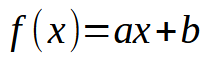
In the initial articles on neural networks, I demonstrated how we could compel the machine to formulate a linear equation. Initially, this equation was constrained to pass through the origin of the Cartesian plane, meaning the line necessarily intersected at the point (0, 0). This was because the constant < b > in the equation below was set to zero.

Although we employed the least squares method to derive a suitable equation, ensuring that the dataset or prior knowledge stored in the database could be appropriately represented in mathematical form, this modeling approach did not help us find the most suitable equation. This limitation arose because, depending on the dataset in the knowledge base, we would need the constant < b > to have a value different from zero.

If you carefully review those previous articles, you will notice that we had to employ certain mathematical maneuvers to determine the best possible values for both the constant < a >, which represents the slope, and the constant < b >, which denotes the intercept. These adjustments enabled us to find the most appropriate linear equation. We explored two methods to achieve this: one through derivative calculations and the other through matrix computations.

However, from this point forward, such calculations will no longer be useful. This is because we need to devise an alternative method for determining the constants in our linear equation. In the previous article, I demonstrated how to find the constant representing the slope. I hope you enjoyed experimenting with that code because now we are about to tackle something slightly more complex. However, despite being only a bit more challenging, this next step will unlock numerous possibilities. In fact, this might be the most interesting article in our neural network series, as everything that follows will become significantly simpler and more practical.

Why Do People Complicate Things So Much?

Now, my dear reader, before we delve into the code, I want to help you understand a few key concepts. When you begin studying neural networks, you will likely encounter a flood of technical terms - an avalanche, really. I'm not sure why those explaining neural networks tend to overcomplicate something fundamentally simple. In my view, there is no reason for such complexity. However, my purpose here is not to criticize or belittle others but to clarify how things work behind the scenes.

To simplify matters as much as possible, let's focus on a few recurring terms associated with neural networks. The first is weights. This term simply refers to the slope coefficient in a linear equation. No matter how others describe it, the term "weight" fundamentally corresponds to the slope. Another commonly used term is bias. This is not an esoteric concept, nor is it exclusive to neural networks or artificial intelligence. On the contrary, bias simply represents the intercept in a linear equation. Since we are dealing with a secant line, please do not confuse these concepts.

Based on these seemingly complex terms, numerous other technical expressions emerge. In fact, these are just different names for the same things. I will not go into why familiar concepts are given different names. But if, while studying neural networks or anything related to them, you encounter unfamiliar terms, take the time to understand the mathematical formula behind them. You will soon realize that, fundamentally, they are much simpler than they appear.

I say this because many people have a tendency to overcomplicate things.

They take something straightforward and begin adding layers of complexity, embellishments, and unnecessary elements, ultimately making something that anyone could understand seem complicated. In programming and the exact sciences, simplicity is key. When things start getting cluttered with unnecessary additions, distractions, and excessive details, it is best to pause, strip away all the unnecessary complexity, and uncover the underlying truth. Many will insist that the subject is complicated, that one must be an expert in the field to understand or implement a neural network, and that it can only be done using a specific language or tool. However, by now, dear reader, you should have realized that a neural network is not complicated. It's actually quite simple.

Now, let's move on to a new topic. We will understand how to incorporate the constant < b >, which represents the point of intersection, or as some prefer to call it: the bias. This is necessary to adjust the equation of the line so that it more accurately represents the dataset we are using to train our neuron.

The Birth of the First Neuron

For our first neuron to take shape - and once it does, we will no longer need to modify it, as you will soon see - we must first understand what we are working with. Our current neuron behaves as shown in the animation below.

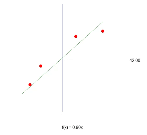
This is the same animation presented in the article Neural Network in Practice: Secant Line. In other words, we have just taken the first step in building a neuron capable of performing a task that was previously done manually using directional keys. However, you may have noticed that this alone is not sufficient. We need to include the intersection constant to further refine the equation. You might assume that doing this is extremely complicated, but it is not. In fact, it is so simple that it almost feels trivial. See below how we add the intersection constant to the neuron. This can be best understood by examining the following fragment.

01. //+------------------------------------------------------------------+
02. double Cost(const double w, const double b)
03. {
04.     double err, fx, x;
05. 
06.     err = 0;
07.     for (uint c = 0; c < nTrain; c++)
08.     {
09.         x = Train[c][0];
10.         fx =  a * w + b;
11.         err += MathPow(fx - Train[c][1], 2);
12.     }
13. 
14.     return err / nTrain;
15. }
16. //+------------------------------------------------------------------+

I am making a point of breaking the code into smaller fragments so that you, dear reader, can understand in detail what is being done. And then, you can tell me: Is it really complicated? Or does it require all the unnecessary complexity that many like to add when discussing neural networks?

Pay close attention because the level of complexity here is almost absurd. (Laughs.) In line nine, we take our training value and assign it to the variable X. Then, in line ten, we perform factorization. Wow! What an incredibly complex calculation! But wait a moment - isn't this the same equation we saw at the beginning? The equation of a straight line? You must be joking! This thing can't possibly function as a neuron used in artificial intelligence programs.

Relax, dear reader. You will see that this will work, just like any other artificial intelligence or neural network program. No matter how complicated people try to make it sound, you will realize that this is fundamentally the same concept implemented in every neural network. The difference lies in the next step, which we will explore shortly. However, the change is not as drastic as you might be thinking. Let's take things one step at a time.

Once the error calculation has been updated, we can modify the fragment responsible for adjusting these two parameters within the cost function. This will be done gradually so that you can grasp some key details. The first step is to modify the original code from the previous article and replace it with the new version shown below.

01. //+------------------------------------------------------------------+
02. void OnStart()
03. {
04.     double weight, ew, eb, e1, bias;
05.     int f = FileOpen("Cost.csv", FILE_COMMON | FILE_WRITE | FILE_CSV);
06. 
07.     Print("The first neuron...");
08.     MathSrand(512);
09.     weight = (double)macroRandom;
10.     bias = (double)macroRandom;
11. 
12.     for(ulong c = 0; (c < ULONG_MAX) && ((e1 = Cost(weight, bias)) > eps); c++)
13.     {
14.         ew = (Cost(weight + eps, bias) - e1) / eps;
15.         eb = (Cost(weight, bias + eps) - e1) / eps;
16.         weight -= (ew * eps);
17.         bias -= (eb * eps);
18.         if (f != INVALID_HANDLE)
19.             FileWriteString(f, StringFormat("%I64u;%f;%f;%f;%f;%f\n", c, weight, ew, bias, eb, e1));
20.     }
21.     if (f != INVALID_HANDLE)
22.         FileClose(f);
23.     Print("Weight: ", weight, "  Bias: ", bias);
24.     Print("Error Weight: ", ew);
25.     Print("Error Bias: ", eb);
26.     Print("Error: ", e1);
27. }
28. //+------------------------------------------------------------------+

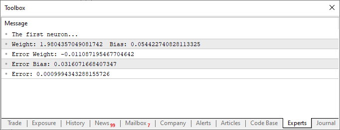
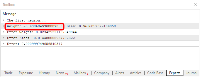
After executing the script with these modifications, you will see something similar to the image below.

Now, let's focus solely on this second code fragment. In line four, we add and modify a few variables - nothing complex. Then, in line ten, we instruct the application to assign a random value to the bias, or our intersection constant. Notice that we also need to pass this value to the Cost function. This is done in lines 12, 14, and 15. However, the interesting part is that we are generating two types of aggregated errors: one for the weight value and another for the bias value. It is important to understand that although both are part of the same equation, they must be adjusted differently. Therefore, we need to determine the specific error each one represents within the overall system.

With this in mind, in lines 16 and 17, we properly adjust the values for the next iteration of the for loop. Additionally, just as we did in the previous article, we also record these values in a CSV file. This allows us to generate a graph and analyze how the values are being adjusted over time.

At this stage, our first neuron is now fully constructed. However, there are still some details that you can grasp by examining the complete code for this neuron, which is provided below. Here is the full code that I came up with.

01. //+------------------------------------------------------------------+
02. #property copyright "Daniel Jose"
03. //+------------------------------------------------------------------+
04. #define macroRandom (rand() / (double)SHORT_MAX)
05. //+------------------------------------------------------------------+
06. double Train[][2] {
07.                     {0, 0},
08.                     {1, 2},
09.                     {2, 4},
10.                     {3, 6},
11.                     {4, 8},
12.                   };
13. //+------------------------------------------------------------------+
14. const uint nTrain = Train.Size() / 2;
15. const double eps = 1e-3;
16. //+------------------------------------------------------------------+
17. double Cost(const double w, const double b)
18. {
19.     double err, fx, a;
20. 
21.     err = 0;
22.     for (uint c = 0; c < nTrain; c++)
23.     {
24.         a = Train[c][0];
25.         fx =  a * w + b;
26.         err += MathPow(fx - Train[c][1], 2);
27.     }
28. 
29.     return err / nTrain;
30. }
31. //+------------------------------------------------------------------+
32. void OnStart()
33. {
34.     double weight, ew, eb, e1, bias;
35.     int f = FileOpen("Cost.csv", FILE_COMMON | FILE_WRITE | FILE_CSV);
36. 
37.     Print("The first neuron...");
38.     MathSrand(512);
39.     weight = (double)macroRandom;
40.     bias = (double)macroRandom;
41. 
42.     for(ulong c = 0; (c < ULONG_MAX) && ((e1 = Cost(weight, bias)) > eps); c++)
43.     {
44.         ew = (Cost(weight + eps, bias) - e1) / eps;
45.         eb = (Cost(weight, bias + eps) - e1) / eps;
46.         weight -= (ew * eps);
47.         bias -= (eb * eps);
48.         if (f != INVALID_HANDLE)
49.             FileWriteString(f, StringFormat("%I64u;%f;%f;%f;%f;%f\n", c, weight, ew, bias, eb, e1));
50.     }
51.     if (f != INVALID_HANDLE)
52.         FileClose(f);
53.     Print("Weight: ", weight, "  Bias: ", bias);
54.     Print("Error Weight: ", ew);
55.     Print("Error Bias: ", eb);
56.     Print("Error: ", e1);
57. }
58. //+------------------------------------------------------------------+

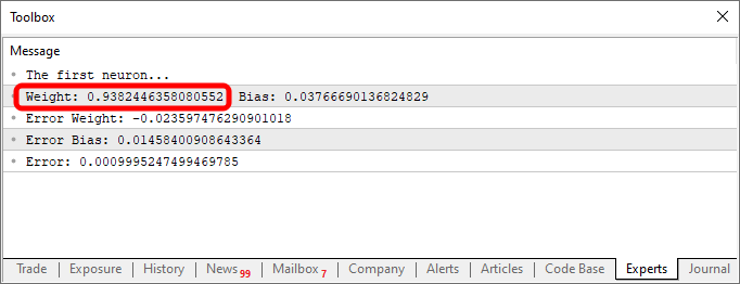
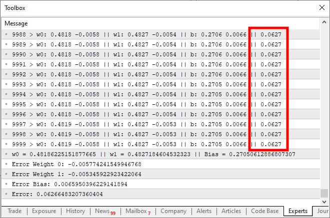
Notice something interesting in both the code and the results shown in the image above. In line six, you can see the values used to train the neuron. Clearly, you can observe that the multiplication factor is two. However, the neuron reports it as 1.9804357049081742. Similarly, we can see that the intersection point should be zero, but the neuron states it as 0.054422740828113325. Now, considering that in line 15, we are accepting an error margin of 0.001, this result isn't too bad. After all, the final error reported by the neuron was 0.0009994343288155726, which is below the threshold we set as acceptable.

These small differences, which you can clearly observe, represent the probability index indicating how close the information is to being correct. This is typically expressed as a percentage. However, you will never see it reach 100%. The number may get very close, but it will never be exactly 100% due to this unavoidable approximation error.

That said, this probability index is not the same as a certainty index regarding the information. At this stage, we are not yet working on generating such an index. We are merely training the neuron and verifying whether it can establish a correlation between the training data. But at this point, you might be thinking: This whole neuron thing is useless. The way you're building it, it serves no real purpose. It just finds a number that we already know. What I really want is a system that can tell me things, generate text, or even write code. Perhaps even a program that can operate in financial markets and make money for me whenever I need it.

Fair enough. You certainly have big ambitions. But if you, dear reader, are looking into neural networks or artificial intelligence purely as a way to make money, I have some bad news for you: you won't succeed that way. The only people who truly profit from this field are those selling AI and neural network systems. They try to convince everyone else that AI can outperform skilled professionals. Aside from these individuals, who will capitalize on selling these solutions, no one else will make money from this alone. If it were that easy, why would I be writing these articles explaining how everything works? Or why would other experts openly share how these mechanisms function? It wouldn't make sense. They could just stay silent and profit from a well-trained neural network. But that's not how things work in reality. So forget the idea that you can throw together a neural network, grab some code snippets here and there, and instantly start making money without any real knowledge.

That said, nothing stops you, my esteemed reader, from developing a small neural network to assist you in decision-making, whether for buying, selling, or simply for better visualizing certain trends in financial markets. Is it possible to achieve this? Yes. By studying everything necessary, even at a slow pace and with significant effort and dedication, you can train a neural network for this purpose. But as I just mentioned, you will need to put in the effort. It is entirely achievable, but not without work.

Now, we have successfully built our first neuron. But before you get too excited and start thinking of ways to use it, let's take a closer look at how it is structured. To make things clearer, look at the image below.

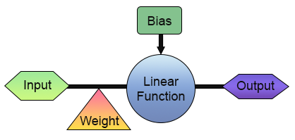
In the image above, we can see how our neuron is implemented. Notice that it consists of one input and one output. This single input receives a weight. At first glance, this might not seem very useful. What's the point of having just one input and one output? I understand your skepticism about what we've just built. However, depending on your background and knowledge in different fields, you may not be aware that in digital electronics, there are circuits that function in exactly this way: with a single input and a single output. In fact, there are two such circuits: the inverter and the buffer. Both are integral components of even more complex systems, and our neuron can actually be trained to replicate their behavior. To achieve this, all you need to do is modify the training matrix, as shown below.

//+------------------------------------------------------------------+
#property copyright "Daniel Jose"
//+------------------------------------------------------------------+
#define macroRandom (rand() / (double)SHORT_MAX)
//+------------------------------------------------------------------+
double Train[][2] {
                    {0, 1},
                    {1, 0},
                  };
//+------------------------------------------------------------------+
const uint nTrain = Train.Size() / 2;
const double eps = 1e-3;
//+------------------------------------------------------------------+

Using this code, you will get something similar to what is shown in the image below:

Note that the weight value is negative, meaning that we will be investing in the input value. In other words, we have an inverter. Using the code below, we can get a different output.

//+------------------------------------------------------------------+
#property copyright "Daniel Jose"
//+------------------------------------------------------------------+
#define macroRandom (rand() / (double)SHORT_MAX)
//+------------------------------------------------------------------+
double Train[][2] {
                    {0, 0},
                    {1, 1},
                  };
//+------------------------------------------------------------------+
const uint nTrain = Train.Size() / 2;
const double eps = 1e-3;
//+------------------------------------------------------------------+

Output, in this case, is shown in the image below.

Notice that now the weight value is positive. This implies that we are buffering the input directly to the output. In other words, we have a buffer. See how fun it is to experiment with this?

The simple act of changing the data in the knowledge base, which, in our case, is a two-dimensional array, allows the same code to generate an equation that represents different behaviors. This is precisely why everyone interested in programming enjoys working with neural networks. They are incredibly fun to experiment with.

That being said, this first neuron is quite limited. Not because of its structure, but because it only allows for a single input. In practice, neurons in neural networks can have as many inputs as needed. Similarly, they can have as many outputs as required to perform their tasks. I am introducing these concepts gradually so that you don't feel overwhelmed. My goal is to help you understand how and why this mechanism works. Of course, no matter how much I or anyone else try to explain, it will never be possible to showcase everything that can be done with this technology. That's because the possibilities are only limited by your creativity. But for now, let's make things a little more interesting and even more fun.

The Sigmoid Function

From this point on, everything I introduce will be just the tip of the iceberg. No matter how exciting, complex, or enjoyable it seems to program, absolutely everything from now on will only be a small glimpse of what's possible. So, my dear reader, at this stage, you should begin studying this subject a bit more independently. My goal is simply to guide you along a path that serves as inspiration for further discoveries. Feel free to explore, experiment, and have fun with what I will show next. As I mentioned earlier, the only real limitation is your imagination.

To allow our single neuron to learn with multiple inputs, you only need to understand one simple but crucial detail. This is illustrated in the image below.

In short, the same equation is given below.

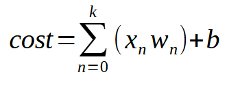
The value < k > represents the number of inputs that our neuron can have. This means that regardless of the number of inputs needed, all we have to do is add the required number of inputs, allowing the neuron to learn how to handle each new situation. However, once we introduce a second input, the function is no longer a linear equation (a straight line). Instead, it becomes an equation capable of representing any possible shape. This change is necessary so that the neuron can adapt to a variety of training scenarios.

Now, things are getting serious. With this adjustment, a single neuron can now learn multiple different patterns. However, there is a small challenge that comes with moving beyond simple linear equations. To understand this, let's modify our program as shown below:

//+------------------------------------------------------------------+
#property copyright "Daniel Jose"
//+------------------------------------------------------------------+
#define macroRandom (rand() / (double)SHORT_MAX)
//+------------------------------------------------------------------+
double Train[][3] {
                    {0, 0, 0},
                    {0, 1, 1},
                    {1, 0, 1},
                    {1, 1, 1},
                  };
//+------------------------------------------------------------------+
const uint nTrain = Train.Size() / 3;
const double eps = 1e-3;
//+------------------------------------------------------------------+
double Cost(const double w0, const double w1, const double b)
{
    double err;

    err = 0;
    for (uint c = 0; c < nTrain; c++)
        err += MathPow(((Train[c][0] * w0) + (Train[c][1] * w1) + b) - Train[c][2], 2);

    return err / nTrain;
}
//+------------------------------------------------------------------+
void OnStart()
{
    double  w0, w1, err, ew0, ew1, eb, bias;

    Print("The Mini Neuron...");
    MathSrand(512);
    w0 = (double)macroRandom;
    w1 = (double)macroRandom;
    bias = (double)macroRandom;

    for (ulong c = 0; (c < 3000) && ((err = Cost(w0, w1, bias)) > eps); c++)
    {
        ew0 = (Cost(w0 + eps, w1, bias) - err) / eps;
        ew1 = (Cost(w0, w1 + eps, bias) - err) / eps;
        eb  = (Cost(w0, w1, bias + eps) - err) / eps;
        w0 -= (ew0 * eps);
        w1 -= (ew1 * eps);
        bias -= (eb * eps);
        PrintFormat("%I64u > w0: %.4f %.4f || w1: %.4f %.4f || b: %.4f %.4f || %.4f", c, w0, ew0, w1, ew1, bias, eb, err);
    }
    Print("w0 = ", w0, " || w1 = ", w1, " || Bias = ", bias);
    Print("Error Weight 0: ", ew0);
    Print("Error Weight 1: ", ew1);
    Print("Error Bias: ", eb);
    Print("Error: ", err);
}
//+------------------------------------------------------------------+

When you run this code, you will get a result similar to the image below:

Now, what went wrong here? Looking at the code, you can see that we only added the possibility of multiple inputs, which was done correctly. However, observe something interesting: around ten thousand iterations, the cost function stops decreasing. Or if it's still decreasing, it's doing so at an extremely slow rate. Why? The reason is that our neuron is missing something. Something that wasn't necessary when we only had a single input, but becomes essential when we introduce multiple inputs. This missing element is also used when working with layers of neurons, a technique applied in deep learning. However, we'll explore that later. For now, let's focus on the main issue. Our neuron is reaching a point of stagnation, where it simply cannot reduce the cost any further. The way to fix this problem is by adding an activation function at the output. The specific activation function and how it behaves depend on the type of problem we are solving. There isn't a single universal solution, and there are many different activation functions we can use. However, the sigmoid function is one of the most commonly used. And the reason for that is simple. The sigmoid function transforms values that range from negative infinity to positive infinity into a bounded range between 0 and 1. In some cases, we modify it to map values between -1 and 1, but for now, we will use the basic version. The sigmoid function is defined by the following formula:

Now, how do we apply this to our code? It might seem complicated at first. But, my dear reader, it’s much simpler than it looks. In fact, we only need to make a few minor changes to the existing code, as shown below:

//+------------------------------------------------------------------+
#property copyright "Daniel Jose"
//+------------------------------------------------------------------+
#define macroRandom (rand() / (double)SHORT_MAX)
#define macroSigmoid(a) (1.0 / (1 + MathExp(-a)))
//+------------------------------------------------------------------+
double Train[][3] {
                    {0, 0, 0},
                    {0, 1, 1},
                    {1, 0, 1},
                    {1, 1, 1},
                  };
//+------------------------------------------------------------------+
const uint nTrain = Train.Size() / 3;
const double eps = 1e-3;
//+------------------------------------------------------------------+
double Cost(const double w0, const double w1, const double b)
{
    double err;

    err = 0;
    for (uint c = 0; c < nTrain; c++)
        err += MathPow((macroSigmoid((Train[c][0] * w0) + (Train[c][1] * w1) + b) - Train[c][2]), 2);

    return err / nTrain;
}
//+------------------------------------------------------------------+
void OnStart()
{
    double  w0, w1, err, ew0, ew1, eb, bias;

    Print("The Mini Neuron...");
    MathSrand(512);
    w0 = (double)macroRandom;
    w1 = (double)macroRandom;
    bias = (double)macroRandom;

    for (ulong c = 0; (c < ULONG_MAX) && ((err = Cost(w0, w1, bias)) > eps); c++)
    {
        ew0 = (Cost(w0 + eps, w1, bias) - err) / eps;
        ew1 = (Cost(w0, w1 + eps, bias) - err) / eps;
        eb  = (Cost(w0, w1, bias + eps) - err) / eps;
        w0 -= (ew0 * eps);
        w1 -= (ew1 * eps);
        bias -= (eb * eps);
        PrintFormat("%I64u > w0: %.4f %.4f || w1: %.4f %.4f || b: %.4f %.4f || %.4f", c, w0, ew0, w1, ew1, bias, eb, err);
    }
    Print("w0 = ", w0, " || w1 = ", w1, " || Bias = ", bias);
    Print("Error Weight 0: ", ew0);
    Print("Error Weight 1: ", ew1);
    Print("Error Bias: ", eb);
    Print("Error: ", err);
}
//+------------------------------------------------------------------+

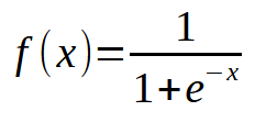
And upon running the above code, the output will resemble the image below:

Take note: it took 2,630,936 iterations for the result to converge within the expected error margin. That's not bad at all. At this point, you might feel like the program is getting a bit slow, especially when running on a CPU. However, this slowdown is primarily due to the fact that we are printing a message at every iteration. A simple way to speed things up is by modifying how we present the output. At the same time, let’s add a small test to evaluate our neuron capability. The final version of the code is shown below:

//+------------------------------------------------------------------+
#property copyright "Daniel Jose"
//+------------------------------------------------------------------+
#define macroRandom (rand() / (double)SHORT_MAX)
#define macroSigmoid(a) (1.0 / (1 + MathExp(-a)))
//+------------------------------------------------------------------+
double Train[][3] {
                    {0, 0, 0},
                    {0, 1, 1},
                    {1, 0, 1},
                    {1, 1, 1},
                  };
//+------------------------------------------------------------------+
const uint nTrain = Train.Size() / 3;
const double eps = 1e-3;
//+------------------------------------------------------------------+
double Cost(const double w0, const double w1, const double b)
{
    double err;

    err = 0;
    for (uint c = 0; c < nTrain; c++)
        err += MathPow((macroSigmoid((Train[c][0] * w0) + (Train[c][1] * w1) + b) - Train[c][2]), 2);

    return err / nTrain;
}
//+------------------------------------------------------------------+
void OnStart()
{
    double  w0, w1, err, ew0, ew1, eb, bias;
    ulong count;

    Print("The Mini Neuron...");
    MathSrand(512);
    w0 = (double)macroRandom;
    w1 = (double)macroRandom;
    bias = (double)macroRandom;

    for (count = 0; (count < ULONG_MAX) && ((err = Cost(w0, w1, bias)) > eps); count++)
    {
        ew0 = (Cost(w0 + eps, w1, bias) - err) / eps;
        ew1 = (Cost(w0, w1 + eps, bias) - err) / eps;
        eb  = (Cost(w0, w1, bias + eps) - err) / eps;
        w0 -= (ew0 * eps);
        w1 -= (ew1 * eps);
        bias -= (eb * eps);
    }
    PrintFormat("%I64u > w0: %.4f %.4f || w1: %.4f %.4f || b: %.4f %.4f || %.4f", count, w0, ew0, w1, ew1, bias, eb, err);
    Print("w0 = ", w0, " || w1 = ", w1, " || Bias = ", bias);
    Print("Error Weight 0: ", ew0);
    Print("Error Weight 1: ", ew1);
    Print("Error Bias: ", eb);
    Print("Error: ", err);

    Print("Testing the neuron...");
    for (uchar p0 = 0; p0 < 2; p0++)
        for (uchar p1 = 0; p1 < 2; p1++)
            PrintFormat("%d OR %d IS %f", p0, p1, macroSigmoid((p0 * w0) + (p1 * w1) + bias));
}
//+------------------------------------------------------------------+

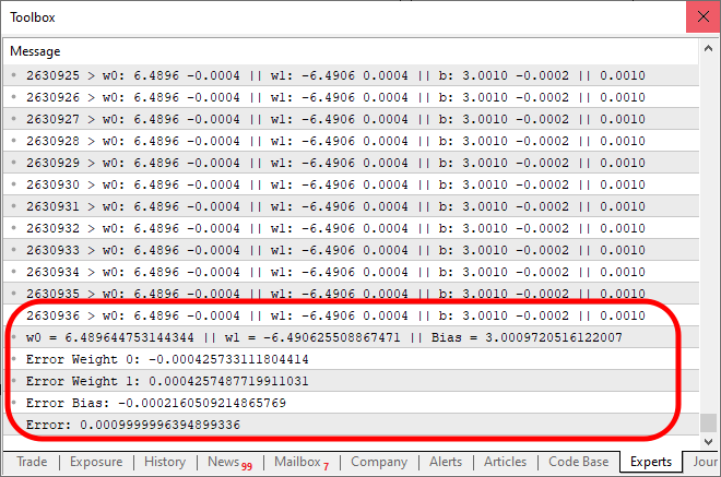
When you execute this updated code, you will see a message similar to the one displayed in the image below, appearing in your terminal:

In other words, we successfully trained our simple neuron to understand how an OR gate functions. At this point, we’ve stepped onto a path of no return. Our single neuron is now capable of learning more complex relationships rather than just detecting whether two values are correlated.

Final considerations

In this article, we built something that often amazes people when they see it in action. With just a few lines of code in MQL5, we created a fully functional artificial neuron. Many believe you need countless resources to accomplish this, but I hope, dear reader, that you now see how things develop step by step. In just a few articles, I've summarized research that has taken years for many scientists to develop. While this neuron is simple, designing the logic behind how it works took a long time. Even today, research continues to make these calculations more efficient and faster. Here, we used only a single neuron with two inputs, five parameters, and one output. And yet, you can see that it still takes some time to find the correct equation.

Of course, we could use OpenCL to accelerate computations via GPU. However, in my view, it's still too early to introduce such an optimization. We can progress further before we truly need GPU acceleration for calculations. That said, if you’re serious about diving deeper into neural networks, I strongly recommend investing in a GPU. It will significantly speed up certain processes in neural network training.

Attached, you'll find the final code from this article. Feel free to use it, experiment with it, and have fun. Observe how this neuron handles various situations, and try to identify its limitations, because they do exist. That's why there's still much more to explore.