Neural Networks in Practice: Stochastic Gradient Descent

Introduction

In my previous article, “Neural Networks in Practice: Gradient Descent”, I showed something that may not have been entirely clear. So, I'll start at that very point. It is important that you, my dear reader, have no doubts about what I am explaining on this topic. The following shows exactly what this is about:

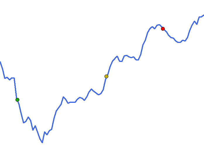
Here's the point: In my previous article, I mentioned that at some point you might have a data set that can be approximated by a blue line. In other words, we have a rather complex polynomial. This polynomial is fed into the neural network so that it can attempt to find an equation capable of describing the data contained in the dataset. So far, I don't think there's anything particularly difficult to understand here. During my explanation, I mention that the points shown in the image represent the magnitude of the error that occurs when the neural network is initialized. And it is precisely this part that may have remained somewhat unclear. I'd like to clarify this point further.

The point is that when we plot something—as many of you have probably seen in explanations involving error—the plot usually represents a surface. The problem is that a surface plot requires two variables: one for the X-axis and the other for the Y-axis. The values corresponding to combinations of these variables are plotted along the Z-axis. Something similar to what is shown in the following animation.

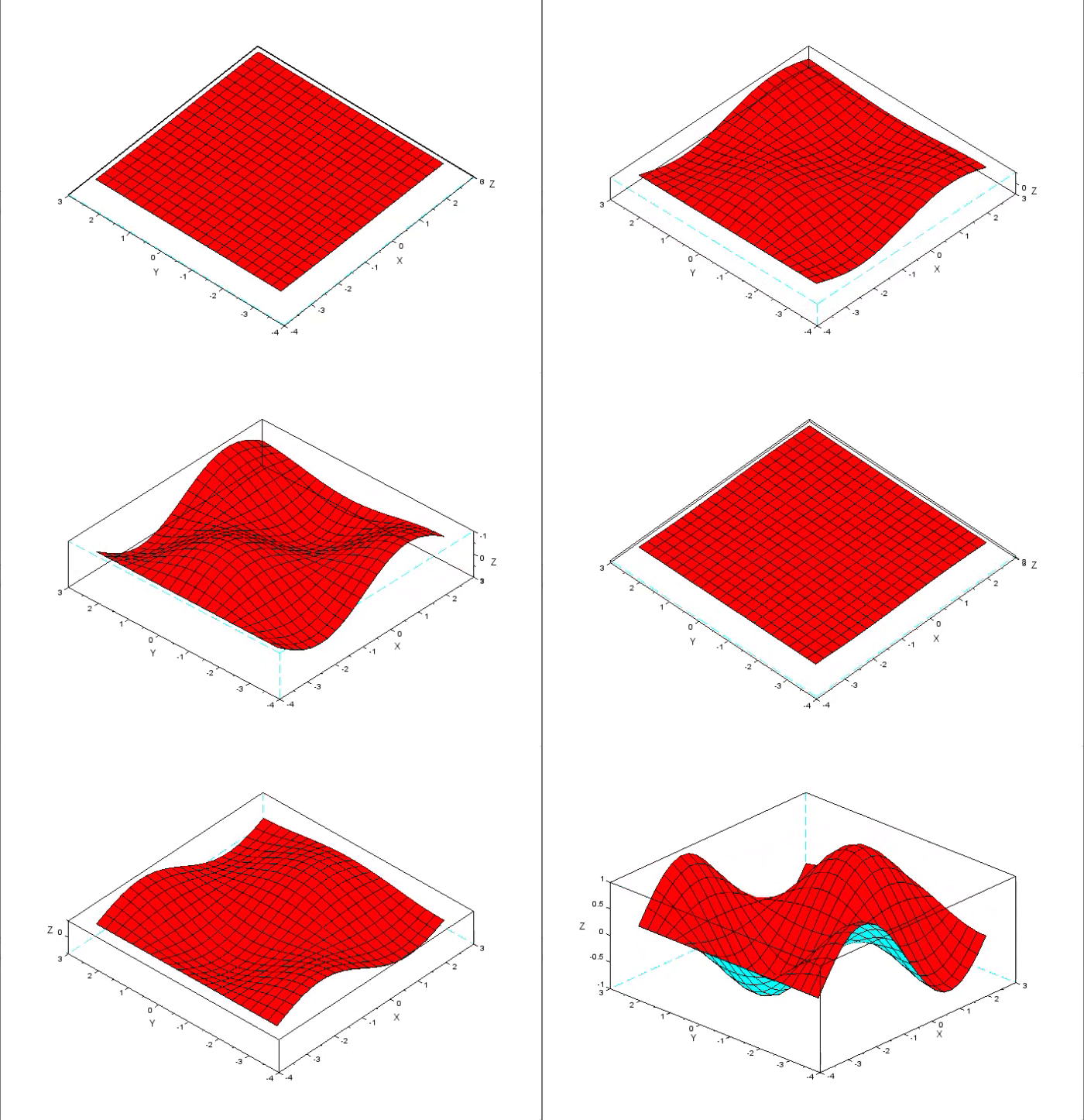
This animation shows that as the values along the Z-axis change, each value along the Z-axis corresponds to a combination of one value along the X-axis and another along the Y-axis. However, the curve shown in the image at the beginning of the article cannot be represented as a surface plot; it is impossible even to imagine what such a plot would look like. This is because constructing it would obviously require far more than two variables.

For this reason, when looking at the curve, it may have been somewhat difficult to understand what the error was. Many people might imagine that a graph representing a data set inherently contains a point where the error is minimal. That's not true. I apologize if I gave that impression, because that is not how it actually works. I simply used a two-dimensional graph to convey the idea of valleys and peaks. We often try to imagine what the perfect valley would look like. However, depending on where we start, we may never be able to reach the point with the smallest error.

I know this seems extremely complicated. And, to be honest, it's really hard to explain, especially since I don't know how familiar each of you is with the math used in neural networks. I try to make the material as simple and easy to understand as possible. It would be much easier to explain it another way. Never mind. I hope I've managed to clarify this issue, which, in my opinion, remained somewhat unclear and could have led to a misunderstanding of the topic.

The code used to create the previous animation is shown below. This is code written for SCILAB—in case anyone is curious and wants to take a closer look at the data.

 t=-%pi:0.3:%pi;
 plot3d(t,t,sin(t)'*cos(t),80,50,'X@Y@Z',[5,2,4]);

If you're interested in exploring this further, you can try running the code above to better understand the concepts of valleys and peaks. To move the 3D graph, press and hold the right mouse button and drag the pointer. All right, now that I think I've clarified the point that was bothering me, we can move on to what we'll be discussing in this article.

Adding a Bias Term to Gradient Descent

Since I have followed a specific methodology from the very beginning, I intend to stick to it in all my articles on neural networks, even though it may sometimes seem as if we are going in circles by returning to the same topics. I’d like to remind you, my dear reader, that neural networks are not a topic with a clearly defined starting point and end goal. When it comes to neural networks, things are much less conventional. Sometimes it seems like we're just getting started, even though we're actually already at the end. Sometimes you may think we’ve reached the end, when in fact we’re only at the beginning. This is rather strange and a bit confusing, especially for those who prefer to begin and end each topic at clearly defined points. As a result, these people give up on studying this topic.

The fact that there is neither a starting point nor an endpoint can be explained simply: neural networks do not have a single solution. Each class of problems involves—or may involve—a completely different solution. Before we move on to these topics, let's look at what was missing to complete the artificial neuron we discussed in the previous article, which used gradient descent. The source code from the previous article is provided in full below.

01. //+------------------------------------------------------------------+
02. #property copyright "Daniel Jose"
03. //+------------------------------------------------------------------+
04. #define PrintEx(A) Print(#A, " => ", A)
05. #define macroRandom (rand() / (double)SHORT_MAX)
06. //+------------------------------------------------------------------+
07. double Train[][2] {
08.                     {0, 0},
09.                     {1, 3},
10.                     {2, 6},
11.                     {3, 9},
12.                     {4, 12},
13.                   };
14. //+------------------------------------------------------------------+
15. const uint nTrain = Train.Size() / 2;
16. const double epsilon = 1e-3;
17. //+------------------------------------------------------------------+
18. double Cost(const double w)
19. {
20.     double err, x, y;
21. 
22.     err = 0;
23.     for (uint c = 0; c < nTrain; c++)
24.     {
25.         x = Train[c][0];
26.         y = Train[c][1];
27.         err += 2 *(x * w - y) * x;
28.     }
29. 
30.     return err;
31. }
32. //+------------------------------------------------------------------+
33. void OnStart()
34. {
35.     double weight, err;
36.     ulong it0, it1, count;
37. 
38.     Print("************************************");
39.     Print("Linear gradient neuron...");
40.     MathSrand(512);
41.     weight = (double)macroRandom;
42. 
43.     it0 = GetTickCount();
44.     for(count = 0; (count < ULONG_MAX) && (MathAbs(err = Cost(weight)) > epsilon); count++)
45.         weight -= (err * epsilon);
46.     it1 = GetTickCount();
47.     Print("Time: ", (it1 - it0) / 1000.0, " seconds.");
48.     PrintEx(count);
49.     PrintEx(weight);
50.     PrintEx(err);
51. }
52. //+------------------------------------------------------------------+

Note that on line 18, where we define the loss function, only the parameter corresponding to the weight is passed to it. And on line 27, where the calculation is performed, we use neither the bias nor its corresponding parameter. I'd like to remind the reader once again that gradient descent is simply a more interesting way to implement linear regression. And that's all there is to it. To better understand this, please refer to the previous articles.

Nevertheless, it has its own advantages over a neuron that performs linear regression. However, simply adding a parameter to account for the bias on lines 18 and 27 does not make the calculation correct. This is because the method for calculating the error will differ slightly from the one used to calculate the error for the bias. You can see this in the following images.

The first figure shows the calculation of the gradient component with respect to the weight; the second figure shows the calculation of the gradient component with respect to the bias. Please note that they differ slightly, as one uses a value that is not present in the other. But this raises another issue related to the code we need to write. Please note that the function returns a value of type `double`, but we need to return two values of type `double`: one for the bias and the other for the weight. Well, if you're already comfortable with MQL5 programming, you won't have any trouble with this. Actually, there are several ways to solve this minor problem. Some of them are easier, while others are a bit more difficult. In any case, I'm not interested in exactly how this problem will be solved.

We are interested in the results obtained. You'll probably notice over time that I approach this problem differently. But I want to make it clear once again that what matters to us is the result itself, not how it is achieved. So, the first way to solve this problem is shown in the following code.

01. //+------------------------------------------------------------------+
02. #property copyright "Daniel Jose"
03. //+------------------------------------------------------------------+
04. #define PrintEx(A) Print(#A, " => ", A)
05. #define macroRandom (rand() / (double)SHORT_MAX)
06. //+------------------------------------------------------------------+
07. double Train[][2] {
08.                     {0, 0},
09.                     {1, 3},
10.                     {2, 6},
11.                     {3, 9},
12.                     {4, 12},
13.                   };
14. //+------------------------------------------------------------------+
15. const uint nTrain = Train.Size() / 2;
16. const double epsilon = 1e-3;
17. //+------------------------------------------------------------------+
18. struct stErr
19. {
20.     double  Weight,
21.             Bias;
22. };
23. //+------------------------------------------------------------------+
24. stErr Cost(const double w, const double b)
25. {
26.     double x, y, t;
27.     stErr err;
28. 
29.     ZeroMemory(err);
30.     for (uint c = 0; c < nTrain; c++)
31.     {
32.         x = Train[c][0];
33.         y = Train[c][1];
34.         t = 2 * ((x * w + b) - y);
35.         err.Weight += (t * x);
36.         err.Bias += t;
37.     }
38. 
39.     return err;
40. }
41. //+------------------------------------------------------------------+
42. void OnStart()
43. {
44.     double weight, bias;
45.     ulong it0, it1, count;
46.     stErr err;
47. 
48.     Print("************************************");
49.     Print("Gradient Descent Neuron...");
50.     MathSrand(512);
51.     weight = (double)macroRandom;
52.     bias = (double)macroRandom;
53. 
54.     it0 = GetTickCount();
55.     for(count = 0; count < ULONG_MAX; count++)
56.     {
57.         err = Cost(weight, bias);
58.         if ((MathAbs(err.Weight) <= epsilon) && (MathAbs(err.Bias) <= epsilon))
59.             break;
60.         weight -= (err.Weight * epsilon);
61.         bias -= (err.Bias * epsilon);
62.     }
63.     it1 = GetTickCount();
64.     Print("Time: ", (it1 - it0) / 1000.0, " seconds.");
65.     PrintEx(count);
66.     PrintEx(weight);
67.     PrintEx(bias);
68.     PrintEx(err.Weight);
69.     PrintEx(err.Bias);
70. }
71. //+------------------------------------------------------------------+

Looking at this code, you might be thinking, “Wow, this is so complicated.” Isn't there an easier way to do this? As I just mentioned, I'm not interested in how it's done. I'm interested in the results. In fact, when you run this code in the MetaTrader 5 terminal, you'll see the following result:

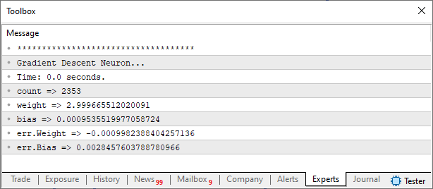
All right, then I'll give a brief explanation for those who just joined us. On line 18, I declare a struct. We will use it to return the calculated error. Notice how the loss function is now declared on line 24. Next, on line 27, we declare a local variable within the function. It will be used to store the values that will be returned. On line 34, we perform the calculations. However, we only calculate a portion of it there. On line 35, we adjust the calculation to include the missing portion in the gradient component with respect to the weight. As a result, we correctly calculate the loss gradients with respect to both the weight and the bias.

There's just one more small issue: the activation function. There are times when the activation function isn't really necessary, while in other cases it is absolutely essential. We've already covered this in an article where I showed how to train a neuron to represent a logic gate. Here, however, since we are using values described by a function that explicitly satisfies the following equation:

the activation function is not needed. Soon we'll have a better understanding of this issue related to the activation function. The only thing you need to understand right now, my dear reader, is that there is no single formula for creating a neural network. Every case is unique. And there are many situations in which a neural network is more of a hindrance than a help. We'll see that very soon, too. Let's not rush things; there's no reason to put the cart before the horse. There's a time for everything.

So, let's get back to our main topic—a neuron that uses gradient descent. You can compile it and run it in the terminal. You'll notice that the results are unchanged from those shown in the previous article. In fact, one of the code snippets included in the appendix to this article is precisely the code for the neuron we just discussed. What will happen if we modify the equation so that we end up with a slightly different equation? What will happen to the neuron, given that its code does not contain an activation function? I want you, my dear reader, to try this experiment. And to help you, let's try out a few different values to arrive at the following equation:

To do this, we need to change some parts of the code.

. //+------------------------------------------------------------------+
07. double Train[][2] {
08.                     {0, -0.8},
09.                     {1, 0.85},
10.                     {2, 2.5},
11.                     {3, 4.15},
12.                     {4, 5.8},
13.                   };
14. //+------------------------------------------------------------------+
                                   .
                                   .
                                   .
41. //+------------------------------------------------------------------+
42. void OnStart()
43. {
                                   .
                                   .
                                   .
55.     for(count = 0; count < 10; count++)
56.     {
57.         err = Cost(weight, bias);
58.         if ((MathAbs(err.Weight) <= epsilon) && (MathAbs(err.Bias) <= epsilon))
59.             break;
60.         weight -= (err.Weight * epsilon);
61.         bias -= (err.Bias * epsilon);
62.         PrintFormat("%I64u > w0: %.4f %.4f || b: %.4f %.4f", count, weight, err.Weight, bias, err.Bias);
63.     }

You can see these changes in the following code snippet: note the places where the code has changed. The first change concerns the data used for training. The next change is in the code for the OnStart procedure. All right, before we look at the result, I want to warn you, my dear reader and enthusiast: we’re using a neuron that might very well just say, “I WON’T BE ABLE TO CONVERGE.”

And if that happens, the loop on line 55 could cause the program to take quite a long time to finish. Since we cannot be certain that the neuron will converge, we need to limit the loop to a small number of iterations. In this case, I'm setting the number of iterations to ten. In each of them, we'll display information about what the neuron is doing. Line 62 is responsible for this. That way, we'll be able to see whether the neuron converges or not. All right, keeping this warning in mind, we can compile and run the modified code.

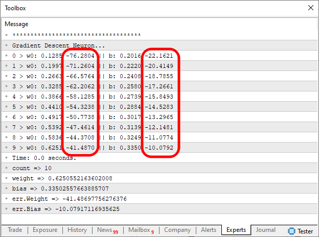
As a result, you will see the following image in the MetaTrader 5 terminal. We are specifically interested in the areas marked in the image. We want their values to approach zero. In fact, they will never reach exactly zero. This is because line 58 will cause the loop to terminate as soon as the error value falls below a preset threshold. This condition must be satisfied simultaneously for both the weight error and the bias error. Otherwise, the loop will continue to run until the specified iteration limit is reached.

Great, we already know that the neuron converges. So let's let it keep trying until either the threshold specified in line 58 or the maximum number of iterations is reached. To do this, we'll replace the value in line 55, currently set to ten, with ULONG_MAX. Or any other value you prefer. As a result, we will get what is shown in the following image:

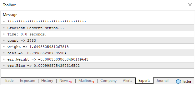
Please note that the result we obtained is very close to what we expected. And we didn't even need to add an activation function for the neuron to converge. Okay, but what if the neuron cannot converge to a result that represents the training data as an equation? What should we do? Every case is unique. There is no rule you have to follow. Or, more precisely, there is no single formula that would ensure that training converges to a mathematical equation describing the data. It is an error to try to follow a specific rule when training a neuron or a neural network. Because THERE IS NO SUCH RULE.

And that is precisely one of the mistakes often made by many people who are just starting to learn about neural networks. They want to follow strict rules at any cost, when in reality we need to understand what we’re actually creating, rather than trying to follow a predetermined formula or use something off the shelf. That is exactly why I am writing these articles on this topic. I am trying to share with you, my dear reader, some of my experience in this area. Perhaps someone will be able to grasp at least some of what I'm showing.

So, before we move on to the next topic, I want to briefly touch on one thing that you may hear more about later. You may have already heard about this, but you probably didn't quite understand what it was all about. I'm talking about what's known as stochastic gradient descent. Yes, that's certainly an imposing term. Just hearing that term alone is enough to send shivers down your spine. At the very least, many people may perceive it that way. But if this applies to you, or if you've never heard of it, there's no need to worry, and you don't have to rush off to find out what it's all about. Stochastic gradient descent is simply a variant of gradient descent. The difference is that this variant is specifically designed to make gradient descent run a little faster.

Okay, so how can we make that happen? This might be interesting to try. Indeed, stochastic gradient descent is a truly interesting method that helps speed up gradient descent. But this comes at a price. There's no such thing as a free lunch. To speed up gradient descent, the stochastic method—I'll call it that so I don't have to keep repeating the full name—uses the following technique. Let's take a look at the code snippet we created to figure this out. It is shown below.

06. //+------------------------------------------------------------------+
07. double Train[][2] {
08.                     {0, -0.8},
09.                     {1, 0.85},
10.                     {2, 2.5},
11.                     {3, 4.15},
12.                     {4, 5.8},
13.                   };
14. //+------------------------------------------------------------------+
15. const uint nTrain = Train.Size() / 2;
16. const double epsilon = 1e-3;
17. //+------------------------------------------------------------------+
18. struct stErr
19. {
20.     double  Weight,
21.             Bias;
22. };
23. //+------------------------------------------------------------------+
24. stErr Cost(const double w, const double b)
25. {
26.     double x, y, t;
27.     stErr err;
28. 
29.     ZeroMemory(err);
30.     for (uint c = 0; c < nTrain; c++)
31.     {
32.         x = Train[c][0];
33.         y = Train[c][1];
34.         t = 2 * ((x * w + b) - y);
35.         err.Weight += (t * x);
36.         err.Bias += t;
37.     }
38. 
39.     return err;
40. }
41. //+------------------------------------------------------------------+

Our training set is fairly small, but imagine if it contained thousands, millions, or maybe even billions of records. If you were to use the code snippet shown above, training just a single neuron could take hours or even days. And that's assuming the dataset would be sufficient to train at least one neuron. If we had to use a neural network, the training time could increase very quickly. All right, now that we understand that, let's see how the stochastic method solves this timing problem.

The magic happens when line 30 is executed. In standard gradient descent, the entire dataset is used each time the loss function is called. In other words, every time the call on line 24 is executed, the loop on line 30 iterates through the entire dataset to train the network—or even just a single neuron. However, research has shown that this is nothing but a waste of time. We can achieve the same result—or, at least, a perfectly satisfactory one—by making a slight modification to this scheme. Instead of using the entire dataset on every iteration—that is, every time the call on line 24 is executed—we will use only a portion of it. At this point, you might be thinking, “But that doesn’t seem very sensible—after all, the training won’t be complete.” However, this impression arises precisely because you, my dear reader, have not yet fully grasped the idea underlying this implementation. Let's see what the code snippet above would look like if we used stochastic gradient descent. It is shown below.

23. //+------------------------------------------------------------------+
24. stErr Cost(const double w, const double b, const uint p1 = 0, const uint p2 = nTrain)
25. {
26.     double x, y, t;
27.     stErr err;
28. 
29.     ZeroMemory(err);
30.     for (uint c = p1; c < p2; c++)
31.     {
32.         x = Train[c][0];
33.         y = Train[c][1];
34.         t = 2 * ((x * w + b) - y);
35.         err.Weight += (t * x);
36.         err.Bias += t;
37.     }
38. 
39.     return err;
40. }
41. //+------------------------------------------------------------------+

Since we only need to change the part responsible for calculating the error, I'm including only the fragment that is actually necessary. Now, perhaps, it will become clearer how the stochastic method works. Please note that changes have been made only to lines 24 and 30. All the rest of the code remains unchanged. There are only two things to keep in mind: first, the value of p1 must be different from p2 and less than p2. Second, the value of p2 must be less than or equal to the number of data points in the training set. Given these conditions, let's see how this can be used.

The calling code can make a certain number of calls to train the system on a set of X elements. Once the network has been trained on these X data points, you move on to the next batch. You then train the model on Y data points, where Y may be equal to or greater than the previous amount. Since the network will already have made some progress in reducing the error, this second training phase will, in many cases, be significantly faster. And so on.

You divide the training data into smaller blocks that can be processed by the loss function much more quickly. For example, let's assume that our dataset contains one million records that will be used for training. If we had to run those one million records through the loss function 100,000 times, it would take an enormous amount of time. Instead, if we ran a batch of 10,000 records through the loss function 100,000 times to reduce the error associated with the weights and bias, the next batch of 10,000 might not need to go through this process 100,000 times. Perhaps about 80,000 iterations would be enough to finish. And the next batch would require even fewer iterations to reduce the error even further. As a result, you use all the training data, but you don't spend as much time as you would if you processed the entire dataset at every iteration.

That is the essence of stochastic gradient descent: to try to reduce the error as quickly as possible. Since you are unlikely to be lucky enough for the pseudorandom generator to assign near-optimal values to the weights and bias, applying this approach to a large dataset is a sensible choice. However, for small datasets—or even the one I’m using to demonstrate how it all works—implementing stochastic gradient descent is completely unnecessary and just takes an enormous amount of time. Therefore, there isn't much point in using it if simpler—and, at first glance, slower—methods can produce good results.

All right. I think we've already covered the topic of stochastic gradient descent, since there isn't really much more to say on the subject. Since we still have a little time left, I can start showing you something that will make more sense in the next article. So let's jump ahead a little. To do that, let's move on to a new topic.

Isn't there another way?

All right, my dear reader. Up until now, everything has progressed gradually and without any major difficulties, which has made it relatively easy to explain many things. It's true, though, that we're still only at the very beginning of everything we can explore. However, since some of the topics we'll be covering are quite difficult to explain in simple terms, I've tried to proceed as slowly and methodically as possible. The idea is to present this topic in a way that's easy to understand, so that everyone can grasp it. Although we've had our ups and downs, I think you were able to follow the explanations and understand the material.

Before moving on to other, somewhat deeper topics, I'd like to clarify something. To do this, we'll need to make a few changes to the neuron code we discussed in this article. There's no need to be afraid or to wonder why. As EN SABAH NUR said: “Everything will become clear in due time, my child.” Now that we understand that, let's take a look at the changes made to the code so I can explain a few things. Again, don't worry about understanding the reason just yet; just take a look at the code below.

001. //+------------------------------------------------------------------+
002. #property copyright "Daniel Jose"
003. //+------------------------------------------------------------------+
004. #include <Canvas\Canvas.mqh>
005. //+------------------------------------------------------------------+
006. #define PrintEx(A)  Print(#A, " => ", A)
007. #define macroRandom (rand() / (double)SHORT_MAX)
008. #define _SizeLine   300
009. #define nColuns     2
010. //+------------------------------------------------------------------+
011. CCanvas canvas;
012. //+------------------------------------------------------------------+
013. double Train[][nColuns] {
014.                     {0, -0.8},
015.                     {1, 0.85},
016.                     {2, 2.5},
017.                     {3, 4.15},
018.                     {4, 5.8},
019.                   };
020. //+------------------------------------------------------------------+
021. const double epsilon = 1e-3;
022. //+------------------------------------------------------------------+
023. struct stErr
024. {
025.     double  Weight,
026.             Bias;
027. };
028. //+------------------------------------------------------------------+
029. stErr Cost(const double w, const double b, const uint p1 = 0, const uint p2 = Train.Size() / nColuns)
030. {
031.     double x, y, t;
032.     stErr err;
033. 
034.     ZeroMemory(err);
035.     for (uint c = p1; c < p2; c++)
036.     {
037.         x = Train[c][0];
038.         y = Train[c][1];
039.         t = 2 * ((x * w + b) - y);
040.         err.Weight += (t * x);
041.         err.Bias += t;
042.     }
043. 
044.     return err;
045. }
046. //+------------------------------------------------------------------+
047. void PlotText(const int x, const int y, const uchar line, const string sz0)
048. {
049.     uint w, h;
050. 
051.     TextGetSize(sz0, w, h);
052.     canvas.TextOut(x - (w / 2), y + _SizeLine + (line * h) + 5, sz0, ColorToARGB(clrBlack));   
053. }
054. //+------------------------------------------------------------------+
055. inline double CallZoom(void)
056. {
057.     double d1 = 0;
058. 
059.     for (uint c = 0; c < Train.Size() / nColuns; c++)
060.     {
061.         d1 = MathMax(d1, MathAbs(Train[c][0]));
062.         d1 = MathMax(d1, MathAbs(Train[c][1]));
063.     }
064. 
065.     return _SizeLine / d1;
066. }
067. //+------------------------------------------------------------------+
068. void Plot_Train2D(const int x, const int y, const double weight, double bias)
069. {
070.     int vx, vy;
071.     double zoom;
072.     uint n = Train.Size() / nColuns;
073. 
074.     zoom = CallZoom();
075.     canvas.LineVertical(x, y - _SizeLine, y + _SizeLine, ColorToARGB(clrRoyalBlue, 255));
076.     canvas.LineHorizontal(x - _SizeLine, x + _SizeLine, y, ColorToARGB(clrRoyalBlue, 255));
077.     for (uint c = 0; c < n; c++)
078.     {
079.         vx = (int)(Train[c][0] * zoom);
080.         vy = (int)(Train[c][1] * zoom);
081.        canvas.FillCircle(x + vx, y - vy, 5, ColorToARGB(clrRed, 255));
082.     }
083.     canvas.LineAA(
084.                 x + (int)(Train[0][0] * zoom), 
085.                 y - (int)((Train[0][0] * weight + bias) * zoom), 
086.                 x + (int)(Train[n - 1][0] * zoom), 
087.                 y - (int)((Train[n - 1][0] * weight + bias) * zoom), 
088.                 ColorToARGB(clrForestGreen));
089.     PlotText(x, y, 1, StringFormat("Zoom: %.2fx", zoom));
090.     PlotText(x, y, 2, StringFormat("f(x) = %.4fx %c %.4f", weight, (bias < 0 ? '-' : '+'), MathAbs(bias)));
091. }
092. //+------------------------------------------------------------------+
093. void OnStart()
094. {
095.     double weight, bias;
096.     int    x, y;
097.     ulong  it0, it1, count;
098.     stErr  err;
099. 
100.     Print("************************************");
101.     Print("Stochastic Gradient Descent Neuron...");
102.     Print("************************************");
103.     MathSrand(512);
104.     weight = (double)macroRandom;
105.     bias = (double)macroRandom;
106. 
107.     it0 = GetTickCount();
108.     for(count = 0; count < ULONG_MAX; count++)
109.     {
110.         err = Cost(weight, bias);
111.         if ((MathAbs(err.Weight) <= epsilon) && (MathAbs(err.Bias) <= epsilon))
112.             break;
113.         weight -= (err.Weight * epsilon);
114.         bias -= (err.Bias * epsilon);
115.     }
116.     it1 = GetTickCount();
117.     Print("Time: ", (it1 - it0) / 1000.0, " seconds.");
118.     PrintEx(count);
119.     PrintEx(weight);
120.     PrintEx(bias);
121.     PrintEx(err.Weight);
122.     PrintEx(err.Bias);
123.     Print("Press ESC to close....");
124.     Print("************************************");
125. 
126.    x = (int)ChartGetInteger(0, CHART_WIDTH_IN_PIXELS, 0);
127.    y = (int)ChartGetInteger(0, CHART_HEIGHT_IN_PIXELS, 0);
128.    canvas.CreateBitmapLabel("BL", 0, 0, x, y, COLOR_FORMAT_ARGB_NORMALIZE);
129.    canvas.Erase(ColorToARGB(clrWhite, 255));
130.     x /= 2;
131.     y /= 2;
132.            
133.     Plot_Train2D(x, y, weight, bias);
134. 
135.    canvas.Update(true);
136. 
137.     while(!IsStopped())
138.         if (TerminalInfoInteger(TERMINAL_KEYSTATE_ESCAPE) !=0)
139.             break;
140. 
141.     canvas.Destroy();
142. }
143. //+------------------------------------------------------------------+

This code will be available in the attached file. I may make some changes before the next article to make it more illustrative. Although I still need to think about whether that will actually be necessary. In any case, when we run it, we'll get the result shown in the following image.

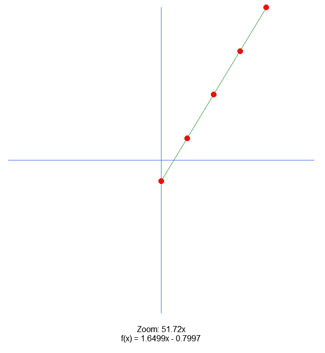
And in the terminal, you'll see the following information:

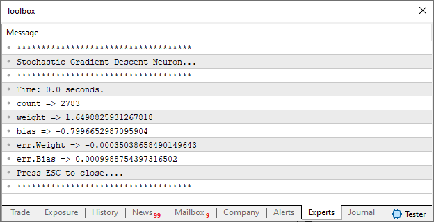
All right, let's see what's going on here. Based on the training data specified on line 13, we use a neuron in the OnStart procedure to derive an equation. This equation will describe a straight line. The neuron will find this equation using gradient descent. However, since the dataset is very small, we will use the simplest method, namely gradient descent. As soon as the neuron signals that it has finished its task, we will display some information in the terminal. This is done in lines 117–124. Next, we'll use the standard CCanvas library to draw a simple graph on the MetaTrader 5 screen. This graph will be created when line 133 is executed, which, in turn, calls the code at line 68.

In the Plot_Train2D procedure, on line 74, we'll ask the application to determine the optimal zoom level for displaying the data, since we may be dealing with very small or very large values. We want all the values to fit within the area where we will place the Cartesian coordinate system. The Y and X axes of the coordinate system are drawn in lines 75 and 76, respectively. Next, on line 77, we enter the for loop. The purpose of this loop is to display all the points used during training. Of course, the points will be positioned correctly according to the scale determined from the values found. All right, next, on line 83, we'll draw a line using the equation found by the neuron. Next, in lines 89 and 90, we display some information about what the graph shows, as well as the image's zoom level.

The goal is to display the data as clearly as possible. This will help you begin to understand what we'll cover in the next article.

Concluding Thoughts

In this article, we have focused primarily on creating a neuron capable of using gradient descent. We also examined a variant of this model called stochastic gradient descent. However, things are not that simple, and there are still some issues to consider.

And here, I'd like you, my dear reader, to try analyzing and experimenting with this last code snippet from the article. But be careful when doing this, since the neuron does not have an activation function. This could cause it to simply reach a plateau. We've seen before that something like this can happen. However, for now, we will not address the issue of activation functions and their true importance. But first, I want to explain something else. And to do that, I need the neuron to remain in its simplest and most basic form. After all, if you understand what we'll discuss in the next article, you'll see that neural networks aren't always the best choice, no matter what anyone tells you.

In the meantime, try changing the training values for this last neuron, whose code will be included in the attached file. Don't change anything else—just the training values. Do this while trying to understand what's going on. This will make it easier to understand what the following articles will cover. However, this article does not address certain issues, which may make it somewhat difficult to understand the mathematical portion. Don't worry; we'll come back to this topic in another article.