

MetaTrader 5 Machine Learning Blueprint (Part 26): Process Permutation
 51
 0

Table of Contents
- Introduction
- What the Deflated Sharpe Ratio Needs Under Adaptive Search
- Permuting the Process, Not the Strategy
- The Trap That Makes the Test Pass When It Should Not
- The Spurious Performance Curve
- Running It on a Real EURUSD Strategy
- Conclusion
- Attached Files
Introduction
Run a hundred trials of a parameter search, keep the best one, and the backtest reports a positive Sharpe ratio. How much of that number came from the market, and how much from keeping the best of a hundred?
This article answers that question for one concrete search. A moving-average crossover is searched over 100 pairs of window lengths on EURUSD H1 data from 2018 through 2024, and the best pair reports an annualized Sharpe of 0.17. The bars are then reshuffled so that no bar carries information about the next, and the same search runs again, 500 times. On the reshuffled data, the search reports a median Sharpe of 0.25.
The real result is lower than what the search typically finds in noise: it sits at the 41st percentile of the reshuffled runs. Repeating the experiment with 20 different sets of parameter pairs does not rescue it. The real result lands between the 31st and 57th percentile each time, and no p-value falls below 0.43. The search found nothing that reshuffled bars could not also produce. Section 6 measures this in full; the sections before it build the tool that does the measuring and the safeguards it depends on.
Part 23 asked whether a feature carries information. Part 24 asked whether a backtest's risk figures survive resequencing. Part 25 asked whether a deployed strategy is still doing what it did in the backtest. None of the three addresses this article's question: how much apparent performance the full development process reports (feature generation, labeling, hyperparameter search, model fitting, and backtest) after inter-bar predictability has been removed from the input. This is a test of the process, not of any one strategy it outputs.
Three terms are kept distinct throughout. Edge means exploitable inter-bar predictability in the real data. Backtest Sharpe means the number a backtest reports, which may or may not reflect edge. Selection effect means the positive backtest Sharpe a search reports on reshuffled bars purely because it keeps the best of many trials. A positive selection effect is expected from any search; the question is whether a real result exceeds it.
This article implements afml.cross_validation.process_permutation:
- permute_development_process runs a complete development pipeline on bar-permuted data and reports the distribution of performance it produces there.
- spurious_performance_curve reports that distribution's median and 90th percentile, with confidence intervals, as a function of trial budget.
- assert_cache_isolation checks that the pipeline responds to its input before a study relies on it.
- quantile_ci gives distribution-free confidence intervals for any null quantile.
This is Part 26, the last of the four-part degradation-avoidance sequence. Its main result is negative for the search it examines, and Section 6 reports it with the uncertainty needed to state it precisely.
What the Deflated Sharpe Ratio Needs Under Adaptive Search
Bailey and López de Prado's Deflated Sharpe Ratio (DSR) corrects a reported Sharpe for selection over many trials, for non-normal returns, and for sample length. It is the correction that any number from Part 9's Bayesian hyperparameter search needs before publication. The selection term takes the number of trials as an input, and the correction is exact only when that number counts independent trials.
TPE, the sampler behind Part 9's Optuna studies, does not produce independent trials. Each trial's parameters are drawn from a distribution fitted to earlier trials, so a hundred TPE trials are sequentially dependent and increasingly concentrated. The trial count DSR needs is then an effective count that has to be estimated, not read off the study. The library already provides an estimator: afml.cross_validation.selection_overfit.effective_trial_count returns the Li and Ji eigenvalue estimate and the Kish design-effect estimate. The difficulty is that the estimates can disagree widely. For the search examined in Section 6, they give 18 and 1.5 effective trials, and the resulting DSR moves from 0.21 to 0.62.
Process permutation answers a different question: it measures the distribution of performance the entire pipeline reports on reshuffled bars for a specific dataset and budget. It does not deflate one reported number under a model of the trials. It needs no trial count, but its answer is only as general as the null it uses (Section 3) and the configuration it was run on. The two methods are complementary, and Section 6 reports both for the same search.
Permuting the Process, Not the Strategy
Two things distinguish this from the earlier permutation tests in this series. First, what gets permuted: not a feature against a target, and not a trade sequence, but the OHLC bars themselves, using the bar_permutation scheme from Part 23. Second, what gets rerun on each permuted copy: not a statistic, but the entire development process.
The null this creates needs to be stated precisely, because it is narrower than "a market with nothing in it". bar_permutation decomposes each bar into an inter-bar gap and an intra-bar body, and shuffles the two sequences independently:
- Preserved: the marginal distribution of gaps.
- Preserved: the marginal distribution of bar bodies, and OHLC consistency within each bar.
- Preserved: the bar count, and the first and last price, so the total drift over the sample.
- Destroyed: autocorrelation and any other inter-bar predictability.
- Destroyed: volatility clustering, so volatility regimes disappear.
- Destroyed: intraday and weekly seasonality, calendar effects, and the ordering of gaps.
The resulting null is that bars are exchangeable. It removes more than predictability: reshuffling eliminates volatility regimes, which can change turnover and path dependence for a moving-average crossover. The test answers a narrower question than whether a strategy family works. It asks whether the process reports more on the real bars than it reports on exchangeable bars with the same marginal distributions.
from afml.cross_validation import permute_development_process

def develop(bars: pd.DataFrame) -> float:
    # feature generation, labeling, HPO, fit, backtest: the WHOLE process
    return run_full_pipeline_and_return_sharpe(bars)

result = permute_development_process(develop, real_bars, n_perm=500, trial_budget=100)
result.spurious_center                    # null median: what the process reports on exchangeable bars
result.median_ci()                        # distribution-free 95% CI for that median
result.p_value                            # one-sided, right tail, add-one corrected
result.null_percentile, result.robust_z   # where the observed value sits, and how far in null units
result.selection_effect_exceeds(tolerance=0.0)   # lower CI bound of the null median > tolerance
develop_fn must accept bars, not a precomputed feature matrix. A version that takes features holds feature generation fixed and tests only the model-fitting stage. Every stage that could adapt to structure in the data has to be inside the permuted call.
The result exposes several statistics, each answering one question:
- p_value is one-sided (right tail): (1 + #{null ≥ observed}) / (n + 1). Ties count as at least as extreme. The observed arrangement is counted as one of the n + 1 (Phipson and Smyth, 2010), so the smallest attainable value is 1 / (n + 1).
- null_percentile is the mid-rank position of the observed value within the null.
- excess_over_null is the observed value minus the null median. It is a location shift only.
- robust_z divides that excess by the null's scaled median absolute deviation, so two results with the same excess but different null widths are distinguished.
- median_ci and quantile_ci give distribution-free confidence intervals from order statistics. A bound the sample cannot support is reported as infinite rather than clipped.
- selection_effect_exceeds(tolerance, level) is true when the lower confidence bound of the null median lies above a tolerance fixed before the study.
The last of these replaces a cruder check. A searching process always shows some positive null median, because it keeps the best of many trials. That is the selection effect, not a defect. Whether it is too large depends on a tolerance the researcher states in advance, and on whether the median is estimated precisely enough to compare against it.
The Trap That Makes the Test Pass When It Should Not
This series caches aggressively. FunctionVersionStore keys feature generation and cross-validation artifacts on a function version and its inputs. That is right for an ordinary research session, where the same bars are reused across dozens of experiments. It is wrong for a permutation study, whose premise is that the input changes on every replicate.
If a permuted bar frame does not change the cache key at the top of the feature-generation chain, every permuted call can return artifacts computed from the real series. The null then collapses onto the observed value, the excess reads as approximately zero, and the study reports a clean result without having run on anything different from what it started with.
from afml.cross_validation import assert_cache_isolation

assert_cache_isolation(develop, real_bars)   # call this before every permutation study
# RuntimeError: develop_fn returned 0.2 and then 0.3 on the same permuted bar series ...
# RuntimeError: develop_fn returned 0.2 on two different permuted bar series ...
assert_cache_isolation runs two checks. First, it calls the development function twice on the same permuted frame and requires identical results. Second, it calls the function on a different permutation and requires a different result. A stochastic pipeline would otherwise pass the second check vacuously, because its outputs differ whether or not it reads the bars, and its optimizer noise would also be mixed into the null. permute_development_process calls it by default before the first replicate, and it passes on the real strategy in Section 6. The attached tests confirm that a function returning a stored value, and a function with unseeded noise, both fail.
The check is necessary, not sufficient. It catches the complete failure, where one stale result is served regardless of input. It cannot prove that every stage reads the permuted bars: a pipeline with one stale stage and one live stage still returns different values on different inputs, and a coarse metric can coincide on genuinely different inputs. Stronger evidence comes from logging the content hash of the bars at the top of the feature chain and confirming zero cache hits across permuted replicates.
The Spurious Performance Curve
The null depends on the trial budget, so a result is only comparable to a null computed at the same budget. In the experiment in Section 6, the null median rises from 0.06 at five trials to 0.31 at three hundred. That establishes the dependence for this one configuration; it does not establish that budget matters more than the sampler, the search space or the strategy family, which this article does not compare.
from afml.cross_validation import spurious_performance_curve

curve = spurious_performance_curve(
    develop_fn_factory=lambda budget: make_develop_fn(n_trials=budget),
    bars=real_bars, budgets=(5, 25, 100, 300), n_perm=500, include_observed=True,
)
# per budget: null median and 90th percentile with 95% CIs, fraction positive,
# and the observed value's percentile and p-value
Every budget is evaluated on the same permuted series, because the permutation seed is shared across budgets. Differences between budgets are then not confounded with differences between permutation draws.
The curve is specific to the configuration used to compute it: pipeline version, data, sample period, cost model, search space, sampler, seed policy, and budget. It is not a constant to reuse after any of these change. It belongs in the same per-release gate as the full study, recomputed whenever the pipeline changes.
The number of replicates matters as much as the budget. With 25 replicates, the 95% confidence interval for the null median runs from the 8th to the 18th order statistic, and the interval for the 90th percentile has no finite upper bound: the sample cannot bound that quantile from above at all. Section 6 uses 500 replicates per null and shows what 25 and 30 replicates would have reported.
Running It on a Real EURUSD Strategy
The development process is a random search over a moving-average crossover's fast and slow windows. This is a deliberately simple strategy family, and the demonstration uses independent random draws rather than TPE. The point of this section is what the search does to the family, not how good the family is.
Data
The study reads the attached file EURUSD_H1_time_2018-01-01-2024-12-31.parq, the EURUSD H1 series used in Part 24 and Part 25. Its origin and construction:
| Property | Value |
|---|---|
| Source | EURUSD bid and ask tick history (every quote) downloaded from FundedNext's MetaTrader 5 trade server with copy_ticks_range and the COPY_TICKS_ALL flag, then aggregated into hourly time bars |
| Price type | open, high, low, and close are bid-ask midpoints; the file also holds the bid and ask bars, but the study reads only the four midpoint columns |
| Time zone | Broker server time as delivered by the terminal: GMT+2, and GMT+3 during daylight saving; time stamps are timezone-naive and unique |
| Bar construction | Each bar is labeled by its close: the bar labeled 10:00 holds the ticks in [09:00, 10:00); hours with no ticks produce no bar |
| Calendar gaps | Weekends and holidays are absent rather than forward-filled. From August 2024 the history includes Friday's last hour, so those weeks end with a bar labeled Saturday 00:00 (22 bars) |
| Coverage | 43,103 bars, January 2, 2018 00:00 to December 31, 2024 00:00 |
| Checksum | SHA-256 47bebd765c107d4627007ebfcb15ffdb1e3c8be9701ffc2ff46d99560a898fed; the study script records whether the file it reads matches |
The gaps matter for this study in two ways. The close-to-close return of the first bar after a gap carries the whole gap, so weekend moves enter the backtest as single bars. bar_permutation treats each of them as one more inter-bar gap and shuffles it with the others, so on permuted series weekend-sized moves can land anywhere in the week. Outside weekends the file has 19 gaps longer than one hour. Nine are holidays around December 25 and January 1. The other ten are gaps in the history itself: single missing days on March 1 and May 1, 2018 and December 1, 2022, the hours from July 15 to July 17, 2024, and six days in late July 2024 with no 00:00 bar. They are left as delivered.
Development process
The specification is:
- Search space: fast window drawn uniformly from 2 to 39 bars, slow window from 20 to 249 bars. valid_pairs removes every pair with fast ≥ slow before the search starts, so the budget counts draws, not valid pairs: 97 of 100 draws are searched at a budget of 100, and 5 of 5, 25 of 25, and 291 of 300 at the other budgets.
- Position: sign(MA_fast − MA_slow), in {−1, 0, +1}, known at the close of bar t and held over bar t + 1.
- Returns: close-to-close log returns, including weekend and holiday gaps.
- Costs: one basis point times the absolute change in position, so a long-to-short reversal costs two basis points. Spread, swap, slippage and execution delay are not modeled separately.
- Annualization: per-bar mean over standard deviation, times the square root of 6,048 (252 days of 24 hours). The data average 6,158 bars per year. The constant scales real and permuted Sharpe identically, so it changes levels, not comparisons.
- Seed policy: the 100 pairs are drawn once and held fixed for the real run and every replicate, so replicates differ only in the data they see, never in the parameters tried. Every seed is listed below.
- Replicates: 500 per null; 200 per run in the grid, cost, and window-range sensitivity studies.
The window ranges and the cost are demonstration assumptions, not estimates of a tradable configuration. The fast range reaches about a day and a half of H1 bars, and the slow range runs from under a day to about ten trading days, so the search covers short intraday crossovers through multi-day ones. The cost of 1 bp per unit change in position, 2 bp per round trip, is about 2.5 times the file's median quoted spread of 0.80 bp (99th percentile 4.0 bp). It is meant to cover the spread with a margin, not to model a particular broker's commission. Table 4 reruns the budget-100 comparison at other costs and window ranges.
The code below is the search as the attached script runs it, including the filter that removes invalid pairs once, before any bars are read:
GRID_SEED = 1                                                # parameter grid of Tables 1, 2 and 4
COST_BPS = 1.0                                               # demonstration cost: 1 bp per unit change in position
ANN = np.sqrt(252 * 24)


def net_pnl(close: np.ndarray, fast: int, slow: int, cost_bps: float = COST_BPS) -> np.ndarray:
    ret = np.diff(np.log(close), prepend=np.log(close[0]))
    ma_f = pd.Series(close).rolling(fast).mean().to_numpy()
    ma_s = pd.Series(close).rolling(slow).mean().to_numpy()
    pos = np.nan_to_num(np.sign(ma_f - ma_s))                # known at the close of bar t
    turn = np.abs(np.diff(pos, prepend=0.0))
    return pos[:-1] * ret[1:] - turn[:-1] * cost_bps * 1e-4  # held over bar t + 1


def sharpe(pnl: np.ndarray) -> float:
    return float(pnl.mean() / pnl.std() * ANN) if pnl.std() > 0 else -10.0


def make_grid(n_trials: int, seed: int = GRID_SEED) -> list[tuple[int, int]]:
    rng = np.random.default_rng(seed)
    fast, slow = rng.integers(2, 40, n_trials), rng.integers(20, 250, n_trials)
    return [(int(f), int(s)) for f, s in zip(fast, slow)]


def valid_pairs(grid: list[tuple[int, int]]) -> list[tuple[int, int]]:
    return [(f, s) for f, s in grid if f < s]                # 97 of 100 draws for seed 1


def searching_process(n_trials: int, seed: int = GRID_SEED):
    grid = valid_pairs(make_grid(n_trials, seed))            # fixed for the real run and every replicate

    def develop(bars: pd.DataFrame) -> float:
        close = bars["close"].to_numpy(dtype=float)
        return max(sharpe(net_pnl(close, f, s)) for f, s in grid)

    return develop
Seeds
Every random draw in the study comes from one of the following seeds, which are constants in process_permutation_study.py:
| Seed | Value | Used for |
|---|---|---|
| Grid seed | 1 | The 100 drawn pairs behind Tables 1 to 5 and Figures 1 and 2 |
| Permutation seed | 3 | Bar permutations for Tables 1 and 2 (shared by every budget and by the search-free control), the 500- and 30-replicate rows of Table 3, every grid in Figure 3, and every row of Table 4 |
| Small-run seed | 2 | The 25-replicate row of Table 3 |
| Cache-check seed | 1 | The two probe permutations of assert_cache_isolation before Table 2 |
| Sensitivity grid seeds | 1–20 | The 20 parameter grids of Figure 3, each run on permutation seed 3 |
Permutations are drawn sequentially from one generator, so two runs with the same permutation seed share their first replicates: the 30-replicate row of Table 3 consists of the first 30 replicates of the 500-replicate run.
| Budget | Null median (95% CI) | Null 90th percentile (95% CI) | Observed (percentile) |
|---|---|---|---|
| 5 | 0.061 [0.025, 0.089] | 0.497 [0.434, 0.565] | 0.017 (45th) |
| 25 | 0.184 [0.137, 0.229] | 0.623 [0.551, 0.679] | 0.091 (39th) |
| 100 | 0.247 [0.203, 0.286] | 0.657 [0.612, 0.739] | 0.172 (41st) |
| 300 | 0.310 [0.261, 0.347] | 0.707 [0.659, 0.756] | 0.295 (48th) |
Table 1. Null performance and observed performance by trial budget, 500 replicates per budget
Null performance versus trial budget, and the observed result at each budget, on real EURUSD H1 data
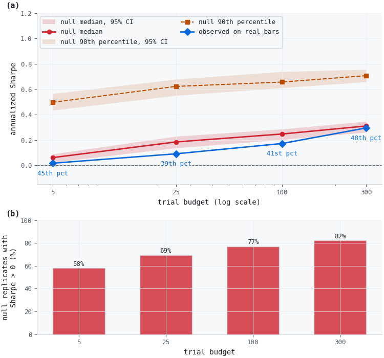
Figure 1. 2-panel illustration of the spurious performance curve on a real MA-crossover search
- (a): the null median (red) and 90th percentile (orange) of the Sharpe the search reports on reshuffled bars, each with its 95% confidence band, and the Sharpe it reports on the real bars (blue), at four budgets. The observed value sits at the 39th to 48th percentile of its null at every budget, below the median each time.
- (b): the share of null replicates reporting a positive Sharpe, rising from 58% at five trials to 82% at three hundred.
A point comparison at a hundred trials, using a search-free control on the same bars:
| Process | Observed | Null median (95% CI) | Percentile, p-value |
|---|---|---|---|
| 100-trial search | 0.172 | 0.247 [0.203, 0.286] | 41st, 0.59 |
| fixed MA(10, 50), no search | −0.384 | −0.435 [−0.471, −0.391] | 56th, 0.45 |
Table 2. Point comparison at a 100-trial budget, 500 replicates each
Permutation null distributions for a searching process and a search-free process on the same real EURUSD bars
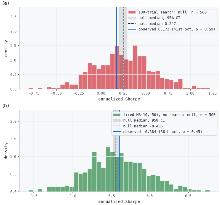
Figure 2. 2-panel illustration of the null each process produces on reshuffled bars
- (a): the hundred-trial search's null across 500 replicates (red), with the null median (dashed), its 95% confidence interval (grey), and the observed Sharpe (blue) at the 41st percentile.
- (b): the fixed, search-free MA(10, 50) process on the same bars (green). Its null median is negative, and the observed value sits at the 56th percentile.
The search's null median is 0.247, with a 95% confidence interval of [0.203, 0.286] that lies entirely above zero, so selection_effect_exceeds(0.0) is true: the search reports a positive Sharpe on reshuffled bars more often than not. The observed 0.172 sits at the 41st percentile of that null (p = 0.59, robust z = −0.23). The excess over the null median is −0.075, and the robust z-score shows it is small relative to the null's spread.
The search-free row is a control, and it supports one specific inference. Same strategy family, same bars, same costs, and no search: its null median is −0.435, with a confidence interval entirely below zero, because costs dominate when nothing is selected. The positive null median of the searching row therefore comes from selection, not from the backtest or the reshuffling. The control does not show that the moving-average family is free of problems. It is a single fixed pair, and it says nothing about that pair's real-world merit.
What 25 and 30 replicates would have reported
The same comparison at the replicate counts often used for expensive pipelines shows why the confidence intervals are not optional:
| Replicates (seed) | Null median | Median 95% CI | 90th percentile 95% CI |
|---|---|---|---|
| 25 (2) | 0.124 | [−0.052, 0.317] | [0.352, ∞) |
| 30 (3) | 0.318 | [0.047, 0.443] | [0.468, ∞) |
| 500 (3) | 0.247 | [0.203, 0.286] | [0.612, 0.739] |
Table 3. Null median of the 100-trial search at three replicate counts
At 25 and 30 replicates, the point estimates of the null median differ by a factor of more than two, and they place the observed 0.172 on opposite sides of the median. Neither run is wrong. Both confidence intervals contain the 500-replicate median, and both are wide enough to say that the median has not been located. Neither interval bounds the 90th percentile from above. A small study that reports only point estimates can support either conclusion.
Sensitivity to the parameter grid
Tables 1 and 2 use one draw of 100 parameter pairs. Drawing 20 different grids and repeating the budget-100 comparison checks whether the result belongs to the search or to one grid:
Observed percentile within its null across 20 independently drawn parameter grids
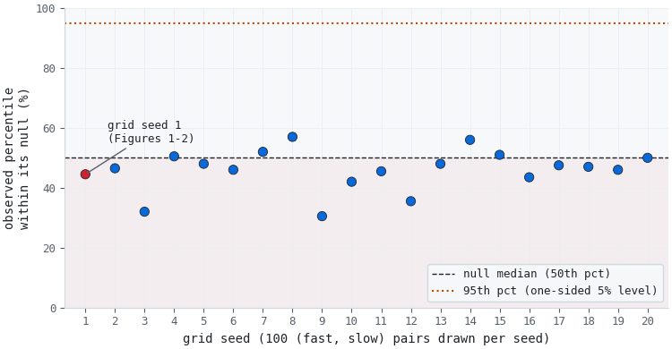
Figure 3. Observed percentile within the permutation null for 20 parameter grids
- Each point is one grid of 100 (fast, slow) pairs, 200 replicates each, with grid seed 1 (used in Figures 1 and 2) in red. The dashed line marks the null median and the dotted line the 95th percentile.
Across the 20 grids, the observed percentile ranges from the 31st to the 57th: below the null median for 14 grids, at it for 1, and above it for 5. The smallest p-value is 0.43. The position below the median in Tables 1 and 2 is a property of grid seed 1, not of the search. The finding that holds across grids is that the real result is indistinguishable from what the search reports on exchangeable bars.
Sensitivity to costs and window ranges
The window ranges and the cost are demonstration assumptions, so the budget-100 comparison is repeated at four cost levels on the baseline ranges, and at 1 bp on a narrower and a wider pair of ranges. Each row uses grid seed 1, permutation seed 3, and 200 replicates.
| Configuration | Observed | Null median (95% CI) | Percentile, p-value |
|---|---|---|---|
| 0 bp, fast 2–39, slow 20–249 (97 pairs) | 0.524 | 0.483 [0.457, 0.530] | 56th, 0.45 |
| 0.5 bp, fast 2–39, slow 20–249 (97 pairs) | 0.275 | 0.321 [0.273, 0.397] | 43rd, 0.57 |
| 1 bp, fast 2–39, slow 20–249 (97 pairs) | 0.172 | 0.206 [0.162, 0.299] | 45th, 0.56 |
| 2 bp, fast 2–39, slow 20–249 (97 pairs) | −0.011 | 0.060 [0.004, 0.131] | 42nd, 0.59 |
| 1 bp, fast 5–20, slow 50–200 (100 pairs) | 0.171 | 0.113 [0.035, 0.151] | 60th, 0.40 |
| 1 bp, fast 2–99, slow 20–499 (94 pairs) | 0.130 | 0.371 [0.308, 0.413] | 20th, 0.81 |
Table 4. Budget-100 comparison at four cost levels and three window ranges, 200 replicates each
Costs move the observed Sharpe and the null together. Without costs the search reports 0.524 on the real bars against a null median of 0.483; at 2 bp the observed value is −0.011 and the null median 0.060. Across the six configurations the observed value sits between the 20th and 60th percentile of its null, and no p-value falls below 0.40. The narrower ranges place it above the null median (60th percentile, p = 0.40) and the wider ranges well below it (20th percentile, p = 0.81). Within these alternatives, the conclusion does not depend on the 1 bp cost or on the chosen ranges. The 1 bp row reruns the Table 2 search with 200 replicates instead of 500, so its null median (0.206) differs from Table 2's (0.247) by Monte Carlo error; each value lies inside the other's confidence interval.
The Deflated Sharpe Ratio on the same search
Because this demonstration draws its trials independently, the DSR applies directly, which makes the two methods comparable on one example. The 97 valid trials produce P&L series with a mean pairwise correlation of 0.66, so the effective trial count is well below 97:
| Trial count used | N | Expected maximum Sharpe | DSR |
|---|---|---|---|
| Raw valid trials | 97 | 0.653 | 0.10 |
| Effective, Li and Ji eigenvalue | 18 | 0.481 | 0.21 |
| Effective, Kish design effect | 1.5 | 0.058 | 0.62 |
Table 5. Deflated Sharpe Ratio of the 100-trial search's best result (0.172 annualized), for three trial counts. Expected maximum Sharpe is annualized
None of the three approaches the conventional 0.95 threshold, so the DSR and the permutation null agree that this result is not evidence of edge. They reach it differently. The DSR's answer moves from 0.10 to 0.62 depending on how the correlated trials are counted, while the permutation null needs no count but is tied to its exchangeable-bars null. Reporting both gives two independent checks with different assumptions.
These results apply only to one instrument, one timeframe, one strategy family, one search space, one sampler, and one cost model. They are not evidence that moving-average crossovers cannot work on EURUSD, and they are not evidence about this series' production pipeline, which conditions its feature search on the screen from Part 23. They are evidence that this hundred-trial search's real-data Sharpe of 0.17 is typical of what the same search reports on exchangeable bars, and that a result of that size from this process should not be reported as evidence of edge.
Conclusion
Key findings:
- Budget parity is not optional. The permuted runs must use the exact trial budget the real run used. Reducing it to save compute changes the quantity being measured.
- Report the precision of the null, not only its center. At 25 replicates the 90th percentile cannot be bounded from above, and two small runs of the same search placed the observed value on opposite sides of the median.
- State the null precisely. Bar permutation produces exchangeable bars. It removes volatility clustering and seasonality along with predictability, so it is not a general model of a market with nothing to find.
- A positive null median is a selection effect, not a verdict. Fix a tolerance in advance and test it against the lower confidence bound of the median.
- Read the excess together with the p-value, percentile and robust z. The excess is a location shift and ignores the null's width.
- Treat the cache check as necessary, not sufficient. Require determinism first, then responsiveness, and log content hashes and cache hits for stronger evidence.
- Rerun the study when the configuration changes. Pipeline version, data, period, costs, search space, sampler, seed policy and budget all shape the null.
- Check seed sensitivity before writing a headline. Across 20 grids, the observed percentile ranged from the 31st to the 57th.
- Label demonstration assumptions and vary them. Across four cost levels and three window ranges, the observed percentile ranged from the 20th to the 60th.
- Use the permutation null alongside the DSR, not instead of it. They answer different questions under different assumptions, and they agreed here.
This closes the four-part degradation-avoidance sequence that began with Part 23. The four tools do not stack into a single pass-fail gate; they answer four separate questions, and clearing three of them says nothing about the fourth.
Attached Files
| File | Module | Description | |
|---|---|---|---|
| 1. | __init__.py | afml.cross_validation | Package exports, adding quantile_ci. |
| 2. | process_permutation.py | afml.cross_validation | ProcessPermutationResult, quantile_ci, assert_cache_isolation, permute_development_process, spurious_performance_curve. |
| 3. | process_permutation_study.py | Script | The EURUSD study: point comparison, budget curve, grid-seed sensitivity, cost and window-range sensitivity, and DSR. Reproduces Tables 1 to 5 and records the data checksum and all seeds. |
| 4. | process_permutation_figures.py | Script | Draws Figures 1 to 3 from the results file the study writes. |
| 5. | test_process_permutation.py | Tests | Tests for the confidence intervals, the result statistics, the cache check and the end-to-end behavior on synthetic noise. |
| 6. | EURUSD_H1_time_2018-01-01-2024-12-31.parq | Data | EURUSD H1 bars, January 2, 2018 to December 31, 2024 (43,103 bars), read by the study. |
| 7. | requirements.txt | Third-party packages the scripts and tests import. | |
| 8. | afml/ (261 other files) | afml | Files from the previous version of the project, as of Part 25. |
The archive contains everything the study, the figures and the tests need. Extract it into MQL5/Files and install the packages with pip install -r requirements.txt (TA-Lib also needs its C library). Run the scripts from MQL5/Files: python afml/process_permutation_study.py (about 30 minutes on one core), then python afml/process_permutation_figures.py, and python -m pytest afml/test_process_permutation.py -q for the tests.
Further Reading
- López de Prado, M. (2018). Advances in Financial Machine Learning. John Wiley & Sons.
- Masters, T. (2020). Permutation and Randomization Tests for Trading System Development.
- Bailey, D. H., & López de Prado, M. (2014). The deflated Sharpe ratio: correcting for selection bias, backtest overfitting, and non-normality. The Journal of Portfolio Management, 40(5), 94–107.
- Phipson, B., & Smyth, G. K. (2010). Permutation p-values should never be zero: calculating exact p-values when permutations are randomly drawn. Statistical Applications in Genetics and Molecular Biology, 9(1), Article 39.
- Li, J., & Ji, L. (2005). Adjusting multiple testing in multilocus analyses using the eigenvalues of a correlation matrix. Heredity, 95(3), 221–227.
Warning: All rights to these materials are reserved by MetaQuotes Ltd. Copying or reprinting of these materials in whole or in part is prohibited.
This article was written by a user of the site and reflects their personal views. MetaQuotes Ltd is not responsible for the accuracy of the information presented, nor for any consequences resulting from the use of the solutions, strategies or recommendations described.


