

Neural Networks in Trading: Temporal Motion Aggregation (Conclusion)
 267
 0

Introduction
Financial markets are like a living organism, pulsing to the rhythm of expectations, fear, and hope. Quote streams, like blood in the veins of the system, carry information encoded in every price movement, every surge of liquidity, and every minor fluctuation that, to an outside observer, may seem random. However, a careful observer knows that nothing here is random. There are only patterns hidden within the chaos. It is precisely this fine line between noise and structure that the Temporal Motion Aggregation (TMA) framework — one of the most interesting and conceptually fresh approaches to time-series analysis to emerge in recent years — seeks to capture this fine line between noise and structure.
The main idea behind TMA is not to view a data sequence as a static stream of values, but to perceive it in terms of movement dynamics, where what matters is not the numbers themselves, but their changes and interrelationships over time. This movement through time is the foundation of the entire architecture. Here, the focus is not on forms, but on pace. Not on points, but on transitions. Not on the data themselves, but on the energy of their movement. On the one hand, this approach is closer to a physical understanding of the market as a system of forces; on the other hand, it is deeply mathematical, as it operates within a space of temporal patterns that can be processed and combined into larger structures describing price behavior.
Architecturally, the framework is built around modules for preprocessing, analysis, and aggregation. At the first level, data is filtered and normalized, bringing it to a common rhythm and scale. Redundant copying and delays are also eliminated at this level to ensure the cleanest possible stream of information. The second level is responsible for forming basic movement patterns — the building blocks of market dynamics. It is here that the system learns to recognize the simplest forms of transitions, upon which more complex structures are then built. Finally, the third level brings all of this together into a single whole — it aggregates patterns to create generalized representations of price movement that can be used for forecasting and making trading decisions.
What sets TMA apart is that it operates not on instantaneous states, but on continuity. In traditional neural network architectures, each time step is treated separately as a static vector of input data. In TMA, the model takes into account the smoothness of transitions, as well as the direction and rate of change. This makes the model sensitive to those hidden rhythms that often elude standard algorithms. In essence, TMA constructs a new perceptual space in which time becomes a structural axis and movement becomes a meaningful unit of analysis.
To put it simply, the TMA framework can be thought of as a bridge between the world of classical time series and the concept of spatial dynamics. It combines a physical sense of market flow with the mathematical rigor of analysis. This is where its unique strength lies. This architecture does not just predict — it explains. It helps you understand why the price moves the way it does and not otherwise. Why certain movements recur while others disappear. Why the market sometimes behaves like a living organism that reacts to internal impulses rather than external events.
The author's visualization of the TMA framework is shown below.
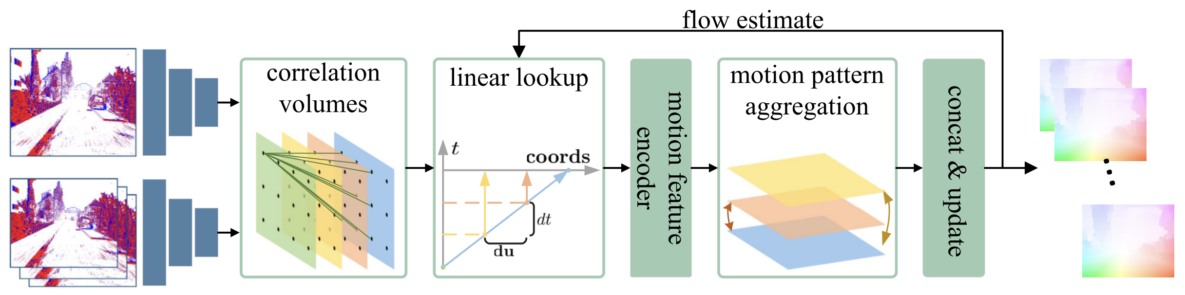
For us, as researchers and developers, TMA has become a starting point for finding new solutions in the field of algorithmic forecasting. Implementing this approach using MQL5 makes it possible not only to test the viability of the authors' ideas but also to adapt them to the real-world conditions of trading systems.
In previous articles, we have already progressed step by step from the theoretical foundations to the practical implementation of the key modules of TMA. We have developed a system capable of processing streams of price changes, structuring them, and extracting meaningful units of movement, which are subsequently combined into aggregated forms. This is not just data processing — it is an intelligent reconstruction of market dynamics. A system built on TMA principles is like an observer who does not record individual events but senses the overall melody of movement. It is able to discern structure where most people see only random fluctuations.
Top-level Object
It should be noted that the TMA architecture did not emerge in a vacuum. It is based on an idea proposed by the authors of the RAFT (Recurrent All-Pairs Field Transforms) framework, which we discussed earlier. RAFT introduced an elegant recurrent processing scheme in which motion is viewed as a continuous field of correspondences between frames in optical flow. This principle turned out to be surprisingly close to the nature of the financial market, where each new price value does not exist in and of itself, but is linked to a multitude of previous states.
Our interpretation of RAFT's ideas has shown just how versatile the concept of a recurrent correspondence field is. It is precisely this that makes it possible to integrate temporal dynamics into a single structure. Here, each new iteration refines the perception of motion, and the model learns to recognize the cause-and-effect relationship between changes.
As with our interpretation of the RAFT framework, the final stage in implementing the approaches proposed by the authors of TMA is the creation of a top-level object — the central element that integrates all previously constructed components into a single, coherent system. At this level, the architecture takes its complete form. Individual modules are linked into an internally organized structure, where data undergoes a complete cycle of transformations, from raw time series to aggregated representations of motion.
And it is no coincidence that the object developed as part of the RAFT implementation was chosen as the parent class. This type of inheritance allows for the reuse of proven methods and helps maintain continuity in architectural principles. We strive to ensure that each new framework is a natural extension of the previous one. The RAFT approaches provided a reliable foundation for recurrent data processing, efficient module interaction, and working with the OpenCL environment. Therefore, using a well-established parent class makes TMA more robust, modular, and scalable.
class CNeuronTMA  :  public CNeuronRAFT
  {
protected:
   CNeuronAddToStack cStatesStack;
   //---
   virtual bool      feedForward(CNeuronBaseOCL *NeuronOCL) override;
   virtual bool      updateInputWeights(CNeuronBaseOCL *NeuronOCL) override;
   virtual bool      calcInputGradients(CNeuronBaseOCL *NeuronOCL) override;

public:
                     CNeuronTMA(void) {};
                    ~CNeuronTMA(void) {};
   //---
   virtual bool      Init(uint numOutputs, uint myIndex, COpenCLMy *open_cl,
                          uint &units[], uint &chanels[], uint group_size,
                          uint groups, uint segments, uint segment_size, uint levels,
                          uint window_key, uint heads,
                          ENUM_OPTIMIZATION optimization_type, uint batch);
   //---
   virtual int       Type(void)   override const   {  return defNeuronTMA;   }
   //--- methods for working with files
   virtual bool      Save(int const file_handle) override;
   virtual bool      Load(int const file_handle) override;
   //---
   virtual void      SetOpenCL(COpenCLMy *obj) override;
   virtual bool      Clear(void) override;
  };
The CNeuronTMA object being created inherits key RAFT mechanisms but gives them new meaning in line with the tasks of temporal aggregation. A state stack, CNeuronAddToStack, is added to its structure to enable the storage and sequential updating of temporal data, which is particularly important when working with motion streams.
The Init method plays a key role in creating a new object. This is where the model acquires its body — the layer sizes, number of channels, aggregation parameters, depth of the correlation stacks, and even the logic of the recurrent connections are defined. Essentially, this is the stage of assembling the model's body, where each element finds its place and purpose, while OpenCL computational resources are allocated to ensure maximum parallelism and data processing efficiency.
bool CNeuronTMA::Init(uint numOutputs, uint myIndex, COpenCLMy *open_cl,
                      uint &units[], uint &chanels[], uint group_size, uint groups,
                      uint segments, uint segment_size, uint levels, uint window_key,
                      uint heads, ENUM_OPTIMIZATION optimization_type, uint batch)
  {
   if(units.Size() != chanels.Size())
      return false;
   uint layers = units.Size() - 1;
   if(!CNeuronSpikeActivation::Init(numOutputs, myIndex, open_cl, units[layers]*chanels[layers],
                                                                      optimization_type, batch))
      return false;
At the very beginning of the method, the supplied parameters are checked for consistency. The array specifying the number of elements in the analyzed sequence at each level (units) must have the same length as the array specifying the number of channels (chanels). The number of elements in the specified arrays indicates the number of neural network blocks involved in the initial processing of the data being analyzed.
Control is then passed to the method of the same name in the parent class, which is responsible for the overall activation of the module and serves as a kind of interface for external interaction with the model's components.
Once the preparatory work is complete, the construction of the main architecture — the encoder (cEncoder) and the context (cContext) backbone — then begins. Each of them is composed of repeating CNeuronSpikeResNeXtBlock structures. These blocks provide deep convolutional feature extraction and generate a robust representation of the time-series data.
   int index = 0;
   CNeuronSpikeResNeXtBlock*              resblock    = NULL;
   CNeuronSpikeConvGRU2D*                 gru         = NULL;
   CNeuronMultScalStackCorrelBySegments*  correlation = NULL;
   CNeuronTMAMFE*                         mfe         = NULL;
   CNeuronTMAMPA*                         mpa         = NULL;
   CNeuronTransposeRCDOCL*                transpose   = NULL;
   CNeuronBaseOCL*                        neuron      = NULL;
   CNeuronBatchNormOCL*                   norm        = NULL;
//---
   cEncoder.Clear();
   cContext.Clear();
   cCorrelation.Clear();
   cG.Clear();
   cEncoder.SetOpenCL(OpenCL);
   cContext.SetOpenCL(OpenCL);
   cCorrelation.SetOpenCL(OpenCL);
   cG.SetOpenCL(OpenCL);
//---
   for(uint i = 0; i < layers; i++)
     {
      resblock = new CNeuronSpikeResNeXtBlock();
      if(!resblock ||
         !resblock.Init(0, index, OpenCL, chanels[i], chanels[i + 1], units[i], units[i + 1],
                                                 group_size, groups, optimization, iBatch) ||
         !cEncoder.Add(resblock))
        {
         DeleteObj(resblock)
         return false;
        }
      index++;
      resblock = new CNeuronSpikeResNeXtBlock();
      if(!resblock ||
         !resblock.Init(0, index, OpenCL, chanels[i], chanels[i + 1], units[i], units[i + 1],
                                                 group_size, groups, optimization, iBatch) ||
         !cContext.Add(resblock))
        {
         DeleteObj(resblock)
         return false;
        }
      index++;
     }
The encoder is responsible for compressing information, while the context branch handles its recurrent refinement, forming the basis for the module's memory.
Next, a recurrent element called CNeuronSpikeConvGRU2D is added to the architecture — the heart of the context backbone, so to speak, which enables dynamic processing of time series. This block allows the model to take past states into account and adjust the current context based on accumulated information.
   gru = new CNeuronSpikeConvGRU2D();
   if(!gru ||
      !gru.Init(0, index, OpenCL, units[layers], chanels[layers], chanels[layers], optimization, iBatch) ||
      !cContext.Add(gru))
     {
      DeleteObj(gru)
      return false;
     }
   index++;
After the basic streams have been formed, a state stack (cStatesStack) is created to temporarily store a latent representation of historical environment states.
   if(!cStatesStack.Init(0, index, OpenCL, segments, chanels[layers], units[layers], optimization, iBatch))
      return false;
   index++;
This is followed by the CNeuronMultScalStackCorrelBySegments module, which calculates multilevel correlations between segments. This is where the central idea behind TMA originates — identifying movement patterns by comparing multiple time windows.
   correlation = new CNeuronMultScalStackCorrelBySegments();
   if(!correlation ||
      !correlation.Init(0, index, OpenCL, segments, segment_size, chanels[layers],
                                   units[layers], levels, optimization, iBatch) ||
      !cCorrelation.Add(correlation))
     {
      DeleteObj(correlation)
      return false;
     }
   index++;
Next to it is the CNeuronTMAMFE (Multi-Feature Extractor) module, which acts as both a filter and a synthesizer. It combines two types of information — spatiotemporal features of price movements and a matrix of correlations between segments — into a single representation. Its main task is to extract and amplify key features from these streams, emphasizing the relationships between them.
Two arrays are supplied as input: the results of temporal aggregation (stack states) and multiscale correlation data (correlation map). The first array contains compact dynamics vectors — a kind of sequence of frames capturing price movement over time, reflecting successive market states. The second array stores the correlation coefficients between these states, showing which segments of the historical data move in sync and which move in antiphase.
Within MFE, these two sources merge in a coordinated manner. Initially, both streams are normalized and passed through multichannel convolutional filters to extract stable combinations of features. They are then combined. A unified feature field is formed. Now, each point contains information about a local price change and the correlation context. This transforms the data stream into an intelligent motion map — structured and self-contained.
   neuron = new CNeuronBaseOCL();
   if(!neuron ||
      !neuron.Init(0, index, OpenCL, correlation.Neurons() + cStatesStack.Neurons(), optimization, iBatch) ||
      !cCorrelation.Add(neuron))
     {
      DeleteObj(neuron)
      return false;
     }
   index++;
     {
      uint temp[] = { cStatesStack.GetDimension(), correlation.GetDimension() };
      mfe = new CNeuronTMAMFE();
      if(!mfe ||
         !mfe.Init(0, index, OpenCL, segments * units[layers], temp, chanels[layers], optimization, iBatch) ||
         !cCorrelation.Add(mfe))
        {
         DeleteObj(mfe)
         return false;
        }
     }
   index++;
It is complemented by CNeuronTransposeRCDOCL, which permutes the dimensions and ensures that the data is properly aligned for subsequent stages.
   transpose = new CNeuronTransposeRCDOCL();
   if(!transpose ||
      !transpose.Init(0, index, OpenCL, units[layers], segments, chanels[layers], optimization, iBatch) ||
      !cCorrelation.Add(transpose))
     {
      DeleteObj(transpose)
      return false;
     }
   index++;
Two CNeuronTMAMPA (Motion Pattern Aggregation) blocks play a special role. It is through them that the model is able to focus on the truly significant movements amid a multitude of minor changes. After the data undergoes preprocessing, correlation, and aggregation, many fragments remain: some carry the key signal, while others are merely noise. This is where the attention mechanism comes into play.
Each CNeuronTMAMPA block receives input segments that have been formed using the principle of temporal aggregation. These blocks extract from this varied set the patterns that recur most frequently or have the greatest energy of change. These are the parts that can serve as indicators of future price movements. Essentially, they define a weighting mask. Some fragments are amplified, while others are attenuated.
As a result, attention blocks allow the model to set priorities rather than simply process everything indiscriminately. It is as if a highly experienced trader were sitting in front of a monitor and saying: "Here, the movement was significant — remember it; but here, it was just noise — do not take it into account." But the model does this automatically and continuously. In market dynamics, where there is more noise than signal, such a mechanism becomes quite valuable.
   for(int i = 0; i < 2; i++)
     {
      mpa = new CNeuronTMAMPA();
      if(!mpa ||
         !mpa.Init(0, index, OpenCL, chanels[layers], window_key, segments, units[layers],
                                                           heads, optimization, iBatch) ||
         !cCorrelation.Add(mpa))
        {
         DeleteObj(mpa)
         return false;
        }
      index++;
     }
It is important to note that we use two CNeuronTMAMPA blocks in a row. The first block can serve as a primary attention filter — it filters out obvious noise and identifies meaningful fragments. The second block — a deep attention layer — receives the already selected fragments from the output of the first block and performs an even finer selection, amplifying the most important ones and highlighting their interconnections. This creates a double attention-filtering effect, enhancing the model's ability to identify patterns in price dynamics.
Thus, CNeuronTMAMPA implements one of the key ideas of the TMA framework: not simply to aggregate motion, but to identify structures within it that deserve attention and then work specifically with those structures. This allows the model to become more selective and robust to noise, adapt more quickly to changes in market dynamics, and, as a result, forecast prices more effectively.
Next, all branches are combined into a single array of features using cConcatenated.
   transpose = new CNeuronTransposeRCDOCL();
   if(!transpose ||
      !transpose.Init(0, index, OpenCL, segments, units[layers], chanels[layers], optimization, iBatch) ||
      !cCorrelation.Add(transpose))
     {
      DeleteObj(transpose)
      return false;
     }
   index++;
//---
   if(!cConcatenated.Init(0, index, OpenCL, units[layers] * ((segments + 2) * chanels[layers]),
                                                                        optimization, iBatch))
      return false;
   index++;
After that, the second recurrent layer, cGRU, is activated to process the already aggregated data. This stage can be compared to comprehension — the model does not simply memorize the structure of the movement, but begins to understand its evolution over time.
   if(!cGRU.Init(0, index, OpenCL, units[layers], (segments + 2) * chanels[layers], chanels[layers],
                                                                              optimization, iBatch))
      return false;
   index++;
In the final stage, the cResidual residual connection path is formed.
   if(!cResidual.Init(0, index, OpenCL, chanels[0], chanels[layers], units[0], units[layers], optimization, iBatch))
      return false;
   index++;
Recall that, as in the RAFT framework, the central data processing backbone in TMA does not simply interpret the market state, but predicts changes in the analyzed features. Each iteration of the calculations effectively constructs a map of expected dynamics, showing how current structures might transform at the next point in time. This predicted shift results from all modules working together, from correlation and aggregation to attention blocks and recurrent refinement.
The values obtained in this process are not considered in isolation — they are added to the current environment state to form a predicted feature field. Thanks to this approach, the model remains stable even if the market changes its behavior. It does not lose the accumulated structure of features, but gradually refines it. With each new step, the model predicts not an absolute value, but a correction — a subtle shift.
After that, two final components are added to perform the final normalization and stabilize training by preventing shifts in feature distributions.
   neuron = new CNeuronBaseOCL();
   if(!neuron ||
      !neuron.Init(0, index, OpenCL, Neurons(), optimization, iBatch) ||
      !cG.Add(neuron))
     {
      DeleteObj(neuron)
      return false;
     }
   neuron.SetActivationFunction(None);
   if(!neuron.SetGradient(cGRU.getGradient(), true) ||
      !cResidual.SetGradient(cGRU.getGradient(), true))
      return false;
//---
   index++;
   norm = new CNeuronBatchNormOCL();
   if(!norm ||
      !norm.Init(0, index, OpenCL, Neurons(), iBatch, optimization) ||
      !cG.Add(norm))
     {
      DeleteObj(norm)
      return false;
     }
//---
   return true;
  }
Thus, the initialization method fully assembles the multilayer dynamic architecture.
The forward pass algorithm is implemented in the feedForward method, which contains the main loop for propagating data through all components of the TMA framework. It can be viewed as the life cycle of a single packet of information — from the initial market features to the final prediction of a change in state.
The algorithm reflects the idea of step-by-step motion refinement that underlies the philosophy of RAFT and TMA, where each computation is a link in a continuous chain of adaptation.
bool CNeuronTMA::feedForward(CNeuronBaseOCL *NeuronOCL)
  {
   if(!cResidual.FeedForward(NeuronOCL))
      return false;
First, the initial data is projected along the residual connection path. This block generates a kind of reference point onto which all subsequent changes are superimposed. It ensures continuity of perception and serves as a backdrop.
Next, two parallel streams — cEncoder and cContext — are processed. The first generates local features — microstructures of motion that reflect short-term market impulses. Each layer of the encoder sequentially extracts new levels of abstraction, ranging from elementary fluctuations to stable patterns of price change.
   CNeuronBaseOCL* current = NULL;
   CNeuronBaseOCL* prev = NeuronOCL;
   for(int i = 0; i < cEncoder.Total(); i++)
     {
      current = cEncoder[i];
      if(!current ||
         !current.FeedForward(prev))
         return false;
      prev = current;
     }
The second stream, cContext, operates at a deeper level. It connects local features into broader temporal relationships, ensuring continuity of analysis. With each step, the contextual representation becomes smoother and more stable, accumulating the model's memory of previous states.
   prev = NeuronOCL;
   for(int i = 0; i < cContext.Total(); i++)
     {
      current = cContext[i];
      if(!current ||
         !current.FeedForward(prev))
         return false;
      prev = current;
     }
When both streams finish running, the encoder's results are passed to the cStatesStack module. This block accumulates a latent representation of the environment state, creating a temporal stack — a history of motion — that can be analyzed as a whole.
   if(!cStatesStack.FeedForward(cEncoder[-1]))
      return false;
At the same time, a correlation map is generated using CNeuronMultScalStackCorrelBySegments, which calculates how synchronously individual segments of the history move.
   CNeuronMultScalStackCorrelBySegments* correlation = cCorrelation[0];
   if(!correlation ||
      !correlation.FeedForward(cEncoder[-1]))
      return false;
These two structures (the state stack and the correlation coefficients) form the core of further calculations, as they incorporate both the dynamics and the interrelationships between segments.
The next step is to combine the results using the concatenation operation. Here, two sources of information (the state stack and the correlation map) are combined into a single tensor. This combination enables the model to consider motion not only over time but also in the space of interrelationships.
   uint variables = cStatesStack.GetVariables();
   uint segments = cStatesStack.GetStackSize();
   uint dimension = cStatesStack.GetDimension();
   uint corr_dim = correlation.GetDimension();
//---
   prev = cCorrelation[1];
   if(!Concat(cStatesStack.getOutput(), correlation.getOutput(), prev.getOutput(),
              dimension, corr_dim, variables * segments))
      return false;
Next, the dynamics analysis block begins operating, with the MFE and MPA modules activated sequentially within it.
- CNeuronTMAMFE extracts joint features across segments and their correlations, strengthening connections that appear consistently.
- CNeuronTMAMPA adds selective attention to this process, highlighting the most significant movement fragments — those that carry the signal rather than noise.
   for(int i = 2; i < cCorrelation.Total(); i++)
     {
      current = cCorrelation[i];
      if(!current ||
         !current.FeedForward(prev))
         return false;
      prev = current;
     }
Each pass through these blocks refines the representation of the market. It is as if the model is learning to look only where something important is happening.
Next, the streams (cEncoder, cContext, and cCorrelation) are combined again into a single structure. This step can be viewed as a moment of knowledge integration: local features, context, and correlational relationships are brought together into a coherent whole.
   if(!Concat(cEncoder[-1].getOutput(), cContext[-1].getOutput(), cCorrelation[-1].getOutput(),
              cConcatenated.getOutput(), dimension, dimension, segments * dimension, variables))
      return false;
The resulting tensor is passed to cGRU—a recurrent block responsible for temporal refinement of the predicted changes. Here, the model accumulates and updates its memory of the motion, generating a prediction of the dynamics of the next state.
   if(!cGRU.FeedForward(cConcatenated.AsObject()))
      return false;
The final step is to combine the outputs of the GRU and the residual block. This is where the framework's key concept is implemented — adding the predicted increments to the current environment state. The result is a new feature map that reflects the expected evolution of the market.
   current = cG[0];
   if(!current ||
      !SumAndNormilize(cGRU.getOutput(), cResidual.getOutput(), current.getOutput(), cGRU.GetChanels(),
                                                                                   false, 0, 0, 0, 1))
      return false;
Next, normalization and spiking activation are applied to the results, producing a nonlinear transformation that puts the output into a form suitable for further interpretation.
   prev = current;
   for(int i = 1; i < cG.Total(); i++)
     {
      current = cG[i];
      if(!current ||
         !current.FeedForward(prev))
         return false;
      prev = current;
     }
//---
   return CNeuronSpikeActivation::feedForward(prev);
  }
Thus, the feedForward method is an integrated process for modeling market dynamics, in which each module plays its own role. The encoder extracts the shape; the context links it across time; the correlation blocks refine the relationships; and the GRU and residual update bring the model closer to an actual forecast.
Together, all these components form the motion backbone of the TMA framework. Here, information does not just flow forward — it evolves, step by step, forming an increasingly accurate understanding of the patterns of the financial market.
Once the forward pass — during which the model generates its own forecast — is complete, the backward pass begins — a process that is no less important and even more nuanced. Now the system needs to figure out exactly where it went wrong and to what extent each internal transformation affected the final result. That is exactly what the calcInputGradients method does. It turns the error into a source of learning, distributing it across the model's layers like blood through the capillaries of a living organism.
bool CNeuronTMA::calcInputGradients(CNeuronBaseOCL *NeuronOCL)
  {
   if(!NeuronOCL)
      return false;
//---
   if(!CNeuronSpikeActivation::calcInputGradients(cG[-1]))
      return false;
The algorithm begins by checking the received pointer to the source data object to which the error gradient is to be passed. If the object is not initialized, backpropagation is interrupted. This is not merely a technical measure, but a safeguard against disruptions to the learning process. Next, the corresponding algorithms of the parent class — the spiking activation module that completed the forward pass — are invoked. Now it is the first to absorb the impact of the backward signal, assessing how much the actual network output has deviated from the target. This is where the initial error gradient is generated, which then begins its journey down through the model's components.
The next step is to pass this signal through the cG block, which is responsible for final data processing. The loop proceeds from the last layer to the first, calling the CalcHiddenGradients method on each element.
   CNeuronBaseOCL* curr = NULL;
//---
   for(int i = cG.Total() - 2; i >= 0; i--)
     {
      curr = cG[i];
      if(!curr ||
         !curr.CalcHiddenGradients(cG[i + 1]))
         return false;
     }
It is like a chain reaction — each neuron determines to what extent its own contribution brought the model closer to — or, conversely, further away from — the correct answer. The error is gradually decomposed across the layers, shedding redundancy and retaining only its meaningful component.
Next, the gradient descends along the main path of the residual branch, cResidual. Its role can be compared to a compensation system: it corrects accumulated imbalances and balances the influence of adjacent layers. As a result, the model does not readjust itself too abruptly, but instead makes subtle, carefully calibrated adjustments.
   if(!NeuronOCL.CalcHiddenGradients(cResidual.AsObject()))
      return false;
Next, processing begins on the concatenated buffer cConcatenated, which combined the outputs of different streams into a single whole during the forward pass. Now the task is the reverse — to break down the total gradient into its components and assign each stream its share of the responsibility.
   if(!cConcatenated.CalcHiddenGradients(cGRU.AsObject()))
      return false;
//---
   uint variables = cStatesStack.GetVariables();
   uint segments = cStatesStack.GetStackSize();
   uint dimension = cStatesStack.GetDimension();
//---
   if(!cEncoder[-1] || !cContext[-1] || !cCorrelation[-1] ||
      !DeConcat(cEncoder[-1].getGradient(), cContext[-1].getGradient(), cCorrelation[-1].getGradient(),
                cConcatenated.getGradient(), dimension, dimension, segments * dimension, variables))
      return false;
   Deactivation(cContext[-1])
   Deactivation(cCorrelation[-1])
   if(cEncoder[-1].Activation() != None)
      if(!DeActivation(cEncoder[-1].getOutput(), cEncoder[-1].getPrevOutput(),
                       cEncoder[-1].getGradient(), cEncoder[-1].Activation()))
         return false;
This is where the DeConcat operation comes into play. This is not merely a mathematical separation of data, but something like separating a complete symphony into its individual instrumental parts. The error is distributed among the encoder, the context module, and the correlation block — the three key components of the forward pass. The encoder is responsible for extracting features, the context module stores temporal dependencies, and the correlation block identifies relationships between market states. After the streams are split, the context and correlation components are deactivated — a gradual reduction in excess activity to avoid amplifying noise or introducing interference between streams during training.
Next, the focus shifts to the correlation blocks. The backward pass through these blocks resembles the work of an analyst who reviews historical data to determine which relationships have actually proven significant. The model learns to distinguish between genuine patterns and random coincidences.
  for(int i = cCorrelation.Total() - 2; i >= 1; i--)
     {
      curr = cCorrelation[i];
      if(!curr ||
         !curr.CalcHiddenGradients(cCorrelation[i + 1]))
         return false;
     }
After that, deconcatenation is performed again, but this time followed by the summation of the data from the two information streams at the encoder's final layer.
   CNeuronMultScalStackCorrelBySegments* correlation = cCorrelation[0];
   uint corr_dim = correlation.GetDimension();
   if(!DeConcat(cStatesStack.getGradient(), correlation.getGradient(), curr.getGradient(),
                dimension, corr_dim, variables * segments))
      return false;
   curr = cEncoder[-1];
   if(!curr.CalcHiddenGradients(cStatesStack.AsObject()) ||
      !SumAndNormilize(curr.getGradient(), curr.getPrevOutput(),
                       curr.getPrevOutput(), dimension, false, 0, 0, 0, 1))
      return false;
   if(!curr.CalcHiddenGradients(correlation) ||
      !SumAndNormilize(curr.getGradient(), curr.getPrevOutput(),
                       curr.getGradient(), dimension, false, 0, 0, 0, 1))
      return false;
The algorithm then returns to the encoder. Here, the model seems to be reevaluating its own perception of the market: it analyzes which features actually conveyed information and which turned out to be spurious. Each layer of the encoder receives its own portion of feedback and adjusts its internal weights, refining the perception filters.
   for(int i = cEncoder.Total() - 2; i >= 0; i--)
     {
      curr = cEncoder[i];
      if(!curr ||
         !curr.CalcHiddenGradients(cEncoder[i + 1]))
         return false;
     }
   if(!NeuronOCL.CalcHiddenGradients(curr))
      return false;
After that, a similar process takes place within the context block. Here, the model reconstructs temporal connections, as if flipping through recent events and assessing exactly where it lost the causal thread.
   for(int i = cContext.Total() - 2; i >= 0; i--)
     {
      curr = cContext[i];
      if(!curr ||
         !curr.CalcHiddenGradients(cContext[i + 1]))
         return false;
     }
Finally, the method sums the gradients obtained from the various information streams at the level of the source data object. The various branches of the model, each with its own logic, are brought into alignment so that the final update to the weights is consistent.
   CBufferFloat* temp = NeuronOCL.getGradient();
   if(!NeuronOCL.SetGradient(NeuronOCL.getPrevOutput(), false) ||
      !NeuronOCL.CalcHiddenGradients(curr) ||
      !SumAndNormilize(temp, NeuronOCL.getGradient(), temp, 1, false, 0, 0, 0, 1) ||
      !NeuronOCL.SetGradient(temp, false))
      return false;
//---
   return true;
  }
In this way, the calcInputGradients method transforms a dry mathematical operation into a true self-learning process. It does not just distribute the error; it retraces the model's entire line of reasoning in reverse, helping it understand where it went wrong and why. This is precisely what gives the TMA framework its vitality: the system does not just react to data; it analyzes its own actions, learns to identify its weaknesses, and, step by step, makes increasingly accurate predictions.
Model Architectures
We have reached an important milestone. We have completed extensive work on developing all the key components of the TMA framework, integrating them, and unifying them under a single top-level object. Now a new, truly practical phase begins: designing the architecture of trainable models that will not only predict market dynamics but also make actual trading decisions.
At this stage, we are once again following the principle of continuity. As before, the framework is evolving gradually: without unduly disrupting what has come before, but with constant refinement of what has already been created. That is precisely why we use a time-tested architecture, developed as part of the RAFT framework, as our foundation. In the Environment State Encoder, the previously used CNeuronRAFT module is now replaced by a new component: CNeuronTMA. This replacement may seem minor at first glance, but in fact it enables the model to develop a deeper, more multilayered understanding of market processes.
//--- Layer 4
   if(!(descr = new CLayerDescription()))
      return false;
   descr.type = defNeuronTMA;
     {
      uint temp[] = {prev_out,                  // Channels In
                     32,
                     64,
                     128                        // Channels Out
                    };
      if(ArrayCopy(descr.windows, temp) < (int)temp.Size())
         return false;
     }
     {
      uint temp[] = {prev_count,                // Units In
                     128,
                     64,
                     32                         // Units Out
                    };
      if(ArrayCopy(descr.units, temp) < (int)temp.Size())
         return false;
     }
     {
      uint temp[] = {StackSize,                 // Segments
                     4                          // Segment Size
                    };
      if(ArrayCopy(descr.heads, temp) < (int)temp.Size())
         return false;
     }
   descr.window = EmbeddingSize / NHeads;       // Group size
   descr.count = NHeads;                        // Groups
   descr.layers = 3;                            // Levels of Correlation
   descr.window_out = EmbeddingSize / NHeads;   // Dimension K
   descr.step = NHeads;                         // Attention Heads
   descr.optimization = ADAM;
   descr.batch = BatchSize;
   if(!encoder.Add(descr))
     {
      delete descr;
      return false;
     }
   iLatentLayer++;
The TMA block, integrated into the architecture, inherits all the strengths of RAFT — recurrent consistency, noise resilience, and the ability to refine features. And it supplements them with a new mechanism for multilevel aggregation and careful analysis of dynamic patterns.
Testing
Once the architecture of the model to be trained has been finalized and our TMA module has been integrated into the Environment State Encoder, the most critical and exciting part begins — training and practical testing. This is where it becomes clear whether TMA is capable not only of processing data, but also of truly thinking in market terms: recognizing patterns, responding to price movements, and making decisions in the spirit of an experienced trader.
The first stage of training can be compared to a trial performance on the historical stage of the market. We use data for the EURUSD currency pair on the M15 timeframe for the period from January 2024 to June 2025. During this phase, the model is exposed to a rich historical context and learns to recognize underlying patterns: volatility, reactions to news, relationships between key features, and the hidden structure of trends. Here, the framework acts as a systems analyst, developing a solid understanding of the market state. Gradually, the model develops the ability to predict how events will unfold and assess the level of risk for each potential trade.
Next comes a more dynamic phase — online fine-tuning in the MetaTrader 5 Strategy Tester. The model now operates under conditions resembling real-time operation, processing data one candlestick at a time. Every price change presents a new situation that requires a quick and precise response. TMA remains stable during sharp fluctuations, filters out noise, and adjusts the strategy during periods of low liquidity. What was previously learned from historical data is transformed into live behavior — flexible, adaptive, and confident.
The final step is to test the model using new data from July through September 2025. Here, the model is evaluated on unseen data, without any advance hints. All parameters learned during training are loaded without modification. This stage demonstrates the extent to which TMA is capable of generalizing and operating in new market conditions, where past experience helps but does not guarantee success.
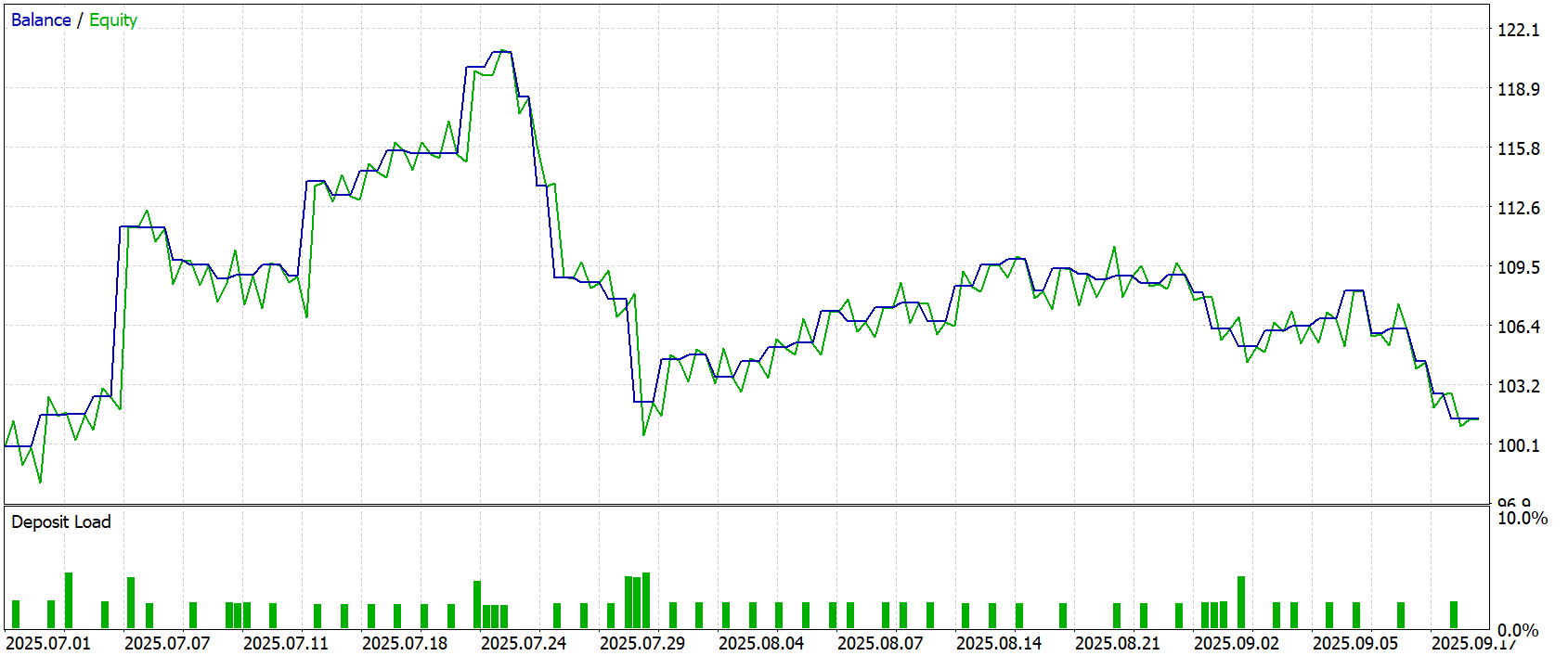
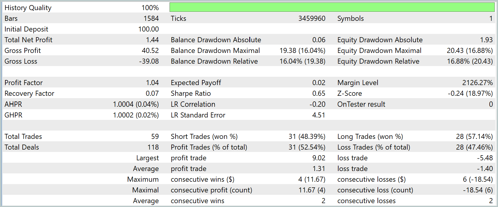
During the three-month test of the TMA framework, the model executed 59 trades, maintaining moderate activity and a balance between long and short positions. This alone indicates that the framework correctly interprets environmental signals, is not prone to overexposure, and operates consistently.
The financial results were modest: a net profit of 1.44% on an initial deposit of USD 100. At the same time, gross profit and loss are virtually balanced (40.52 USD versus –39.08 USD), resulting in a Profit Factor of 1.04 — the break-even threshold. This result is typical for a model that is still in the process of adaptation: it has not yet been optimized for the entry conditions and capital management strategy, but it is already demonstrating stability without catastrophic losses.
A drawdown of 16–17% indicates a moderate level of risk, which is entirely acceptable for the research phase. The balance and equity move in tandem, which confirms that the model closes positions in a timely manner, without a dangerous accumulation of unrealized losses. This is an important indicator of the maturity of the system's internal decision-making logic: the system does not get stuck in losing trades and responds correctly to exit signals.
An analysis of trading sequences also confirms that the trading behavior is balanced: the maximum number of consecutive winning trades is 4, and the maximum number of consecutive losing trades is 6. The proportion of profitable trades (52.5%) is only slightly above the probability threshold, but there is a trend toward symmetry between short and long positions, which indicates that the strategy is neutral — it is not prone to directional biases.
Capital growth follows a wave-like pattern: a period of steady growth in the first half of July is followed by a drawdown and then a phase of stagnation. This is a classic scenario for a model that is still searching for the optimal balance between responsiveness and stability.
Overall, the test results show that the TMA framework is capable of developing its own trading logic, analyzing market data, and making decisions without external support. It successfully passes a key test — it performs consistently without losing control of risk and shows features of an ability to learn. This result can be considered a starting point: the system has proven its viability, and now its task is to improve.
Conclusion
We have completed the development of the TMA framework and conducted initial testing of the model. We can now say with confidence that the architecture we have created not only works but also exhibits all the features of a fully fledged learning system. It analyzes the market, identifies patterns in the data, and makes decisions based on internal logic rather than predefined rules.
Test results showed that the model is already capable of operating consistently in a dynamic environment, maintaining control over risk and avoiding typical overfitting errors. Yes, profits are still modest, but what matters is that TMA has proven the viability of its concept. It was tested using real-world data, proved to be stable, and laid the foundation for further development.
The next step is obvious: in-depth optimization, fine-tuning of parameters, and expansion of behavioral models. More complex systems can be built on this foundation. Our framework has already demonstrated that it is capable of thinking in terms of the future. Now it is time to teach it to act with the confidence of a professional.
Links
Software used in this article
| # | Name | Type | Description |
|---|---|---|---|
| 1 | Study.mq5 | Expert Advisor | Expert Advisor for offline model training |
| 2 | StudyOnline.mq5 | Expert Advisor | Expert Advisor for online model training |
| 3 | Test.mq5 | Expert Advisor | Model testing Expert Advisor |
| 4 | Trajectory.mqh | Class Library | Structure describing the system state and model architectures |
| 5 | NeuroNet.mqh | Class Library | Class library for building a neural network |
| 6 | NeuroNet.cl | Library | Code library for an OpenCL program |
Translated from Russian by MetaQuotes Ltd.
Original article: https://www.mql5.com/ru/articles/20228
Warning: All rights to these materials are reserved by MetaQuotes Ltd. Copying or reprinting of these materials in whole or in part is prohibited.
This article was written by a user of the site and reflects their personal views. MetaQuotes Ltd is not responsible for the accuracy of the information presented, nor for any consequences resulting from the use of the solutions, strategies or recommendations described.

 Neural Networks in Practice: Stochastic Gradient Descent
 Practical Modules from Other Languages in MQL5 (Part 09): MATPLOTLIB (II)
 From Basic to Intermediate: Subwindows (I)
 Confident Learning: Finding Mislabeled Trades Before They Poison Your Classifier

- Free trading apps
- Over 8,000 signals for copying
- Economic news for exploring financial markets
You agree to website policy and terms of use