Feature Engineering for ML (Part 10): Structural Break Tests in MQL5

MetaTrader 5 — Trading systems | 6 July 2026, 11:43

617

Patrick Murimi Njoroge

Introduction

Part 9 of this series implemented the structural break test suite from AFML Chapter 17 in Python, covering the Chu-Stinchcombe-White CUSUM test, the Chow-Type Dickey-Fuller test, SADF across six regression models, and two robustifying variants (QADF and CADF). This article ports the three core tests — CSW, Chow, and SADF — to MQL5 as a single include file, CStructuralBreaks.mqh, placed in MQL5/Include/StructuralBreaks/. The sub- and super-martingale tests (SM-Exp and SM-Power) are included as well, rounding the suite to five statistics per bar.

The MQL5 implementation departs from the Python version in one structural decision that is worth stating immediately: SADF uses a rolling lookback window rather than a full expanding window. In Python, the expanding window is viable because the computation runs once offline on a fixed dataset. In an EA that recalculates on each new bar, an expanding window scales as O(T²) with the number of completed bars. At T = 1,000 bars — a modest two-year daily series — the expanding window performs 15× more inner-loop operations than a 252-bar rolling window. At T = 5,000 bars it performs 400× more. The rolling window is not a compromise; it changes the interpretation of the statistic slightly, and that change is documented in Section 6.

Architecture: CStructuralBreaks

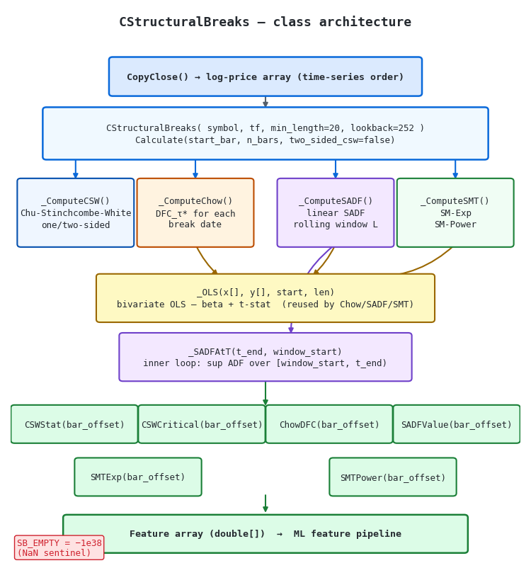
CStructuralBreaks — Class Architecture

Figure 1. Architecture of the CStructuralBreaks class

Input (blue): CopyClose() fills the raw close array, which is immediately log-transformed. All computation works on log-prices throughout; passing a raw price series would produce biased results for the reason explained in Part 9.
Compute methods (teal/orange/purple/green): Each test family is isolated in its own private method. _ComputeCSW() precomputes σ²t via a cumulative sum, then runs the two-pass inner loop. _ComputeChow() builds the Dt[τ*] dummy regressor for each break date. _ComputeSADF() calls the shared _SADFAtT() helper for each endpoint. _ComputeSMT() regresses log-prices on functional forms of time.
OLS accumulation: Each compute method accumulates regression sums inline. Chow uses no-intercept OLS (β = ΣXY / ΣX²) because the Chow specification contains no constant term; residual variance uses df = n − 1. SADF and SMT use intercept-augmented OLS, computing α and β jointly, subtracting both from the residual, and using df = n − 2.
Accessors (green): Six double values per bar indexed by offset from the most recent bar. SB_EMPTY = −1e38 is the sentinel; a result is valid when value > SB_EMPTY + 1.0.

#include <StructuralBreaks\CStructuralBreaks.mqh>

//+------------------------------------------------------------------+
//| EA initialization: create structural breaks engine               |
//+------------------------------------------------------------------+
void OnInit()
  {
   //--- Instantiate with min_length=20 (τ) and lookback=252 (L)
   g_sb = new CStructuralBreaks(_Symbol, _Period, 20, 252);
   if(g_sb == NULL) return(INIT_FAILED);
   return(INIT_SUCCEEDED);
  }

//+------------------------------------------------------------------+
//| New bar handler: compute all statistics and read latest values   |
//+------------------------------------------------------------------+
void OnTick()
  {
   //--- Only process once per new bar
   if(iTime(_Symbol, _Period, 0) == g_last) return;
   g_last = iTime(_Symbol, _Period, 0);

   //--- Calculate for the most recent 300 bars (or less if unavailable)
   if(!g_sb.Calculate(1, 300)) return;

   //--- Retrieve features for the current bar (offset 0)
   double csw_excess = g_sb.CSWStat(0) - g_sb.CSWCritical(0);
   double sadf       = g_sb.SADFValue(0);
   double chow_dfc   = g_sb.ChowDFC(0);
   double smt_exp    = g_sb.SMTExp(0);
   //--- Use these values in regime logic (see Section 9)
  }

Index Convention: The Source of Most Porting Errors

The single most common source of bugs when porting statistical code from Python to MQL5 is the array indexing convention. Python processes data in chronological order: index 0 is the oldest observation, index T−1 is the most recent. MQL5 Copy* functions with ArraySetAsSeries(true) use time-series order: index 0 is the most recent bar, index T−1 is the oldest.

In CStructuralBreaks.mqh, the log-price array is stored in time-series order throughout. The mapping between the two systems is:

//+------------------------------------------------------------------+
//| Index mapping between chronological (Python) and time-series (MT5)|
//+------------------------------------------------------------------+
// Chronological index k ↔ time-series index ts:
//   ts = (n - 1) - k
//   k  = (n - 1) - ts
//
// Price difference in chronological order:
//   dp[k] = chron[k+1] - chron[k]
//         = m_log_p[n-2-k] - m_log_p[n-1-k]   (newer minus older)
//
// In Python (np.diff):
//   dp[k] = log_p[k+1] - log_p[k]              (older to newer)
//
// Both produce the same differences; the loop direction is reversed.

The CSW inner loop, which computes Sn,t = (yt − yn) / (σ̂t √(t−n)), must use the chronological value at position t and compare it against all earlier positions n. In MQL5, position t in chronological space maps to m_log_p[n-1-t]. Getting this conversion wrong does not produce a compile error; it silently computes the statistic on a time-reversed series, which inverts the sign of trending episodes and produces a statistic that rises on downtrends and falls on uptrends.

All four compute methods operate in chronological space and write results to the time-series-indexed output arrays via a single mapping step at the end of each inner iteration. This keeps the statistical logic readable against the chapter formulas while producing the correct time-series-indexed accessor behavior.

Chu-Stinchcombe-White CUSUM

The optimized CSW implementation from the Python module carries over directly to MQL5. The key optimization — precomputing σ²t via a cumulative sum before the inner loop — eliminates the O(n) variance recomputation that makes the naive implementation O(n³) overall:

//+------------------------------------------------------------------+
//| _ComputeCSW: Chu-Stinchcombe-White CUSUM test on levels          |
//|   Precomputes cumulative squared differences, then scans all     |
//|   (n,t) pairs to find the supremum normalized departure.         |
//|   two_sided=true uses absolute differences (symmetric).          |
//+------------------------------------------------------------------+
void CStructuralBreaks::_ComputeCSW(bool two_sided)
  {
   //--- Build sigma² via cumulative sum in chronological order — O(n)
   cum_sq[0] = 0.0;
   for(int k = 1; k < n; k++)
     {
      double dp = m_log_p[n-1-k] - m_log_p[n-1-(k-1)];
      cum_sq[k] = cum_sq[k-1] + dp*dp;
     }

   //--- Outer loop: t from 2 to n-1 (chronological)
   for(int t = 2; t < n; t++)
     {
      double sigma = MathSqrt(cum_sq[t] / (double)(t-1));
      if(sigma <= 0.0) continue;
      double val_t     = m_log_p[n-1-t];
      double max_s     = SB_EMPTY;
      int    best_span = 0;
      //--- Inner loop: n from 0 to t-1 (earlier points)
      for(int nn = 0; nn < t; nn++)
        {
         double diff = two_sided ? MathAbs(val_t - m_log_p[n-1-nn])
                                  : (val_t - m_log_p[n-1-nn]);
         double s = diff / (sigma * MathSqrt((double)(t-nn)));
         if(s > max_s) { max_s = s; best_span = t-nn; }
        }
      //--- Write to time-series index (most recent bar first)
      int ts = n-1-t;
      m_csw_stat[ts] = max_s;
      if(best_span > 0)
         m_csw_crit[ts] = MathSqrt(4.6 + MathLog((double)best_span));
     }
  }

The feature extracted for the ML pipeline is the signed excess over the critical value: CSWStat(0) − CSWCritical(0). Positive values indicate the null of no trend is rejected; negative values indicate the series is within the white-noise bound. The two-sided variant is selected by passing true to Calculate(); it uses MathAbs(val_t − val_n) and is symmetric with respect to rallies and sell-offs.

Chow-Type Dickey-Fuller

The Chow implementation builds the price-diff and lagged-level arrays once per Calculate() call. It then loops over all break dates τ* in [min_length, n − min_length − 1]. For each τ* the dummy regressor Dt[τ*] is zero before τ* and one from τ* onward, so the effective OLS accumulation loop runs only over the active segment [τ*, n−1]:

//+------------------------------------------------------------------+
//| _ComputeChow: Chow-Type Dickey-Fuller with unknown break date    |
//|   For each possible τ*, fits Δy_t = δ·y_{t-1}·D_t[τ*] + ε_t      |
//|   using no-intercept OLS. Stores DFC_{τ*} at time-series index.  |
//+------------------------------------------------------------------+
for(int tau = min_l; tau <= n - min_l - 1; tau++)
  {
   //--- No-intercept OLS: beta = SXY/SXX over active (D=1) segment
   double sxx = 0.0;
   double sxy = 0.0;
   int    cnt = 0;
   for(int k = tau; k < n-1; k++)
     { sxx += lag_c[k]*lag_c[k]; sxy += lag_c[k]*diff_c[k]; cnt++; }
   if(cnt < 4 || sxx < 1e-20) continue;
   double beta = sxy / sxx;

   //--- Residuals over full sample (both segments) with df = n_full - 1
   double ss_res = 0.0;
   int    n_full = 0;
   for(int k = 0; k < n-1; k++)
     {
      double x_d = (k >= tau) ? lag_c[k] : 0.0;
      ss_res += (diff_c[k] - beta*x_d) * (diff_c[k] - beta*x_d);
      n_full++;
     }
   if(n_full < 2) continue;
   double s2    = ss_res / (double)(n_full - 1);
   double var_b = s2 / sxx;   // var(beta) = s²/SXX for no-intercept OLS
   if(var_b <= 0.0) continue;
   double t_stat = beta / MathSqrt(var_b);
   //--- Store t-ratio at the time-series index corresponding to tau
   int ts = n - 1 - tau;
   m_chow_dfc[ts] = t_stat;
  }

The no-intercept specification matches the Chow-Type DFC regression exactly: Δyt = δ · yt−1 · Dt[τ*] + εt contains no constant term. With one estimated parameter the residual degrees of freedom is n − 1, and the variance of the slope estimator is var(β) = σ² / ΣX², without the centering correction that the intercept-adjusted formula requires. Mixing the intercept-adjusted β formula with no-intercept residuals inflates ss_res and deflates the t-statistic.

This separation — X'X from the active segment, residuals from the full sample — matches the Chow-Type specification in the chapter. The t-ratio DFCτ* is stored at the time-series index corresponding to τ*. The supremum SDFC = maxτ* |DFCτ*| can be computed from the full array after Calculate() completes:

//+------------------------------------------------------------------+
//| Compute SDFC and locate the break bar after Calculate()          |
//+------------------------------------------------------------------+
double sdfc      = SB_EMPTY;
int    break_bar = -1;
for(int i = 0; i < g_sb.Count(); i++)
  {
   double v = g_sb.ChowDFC(i);
   if(v > SB_EMPTY + 1.0 && MathAbs(v) > MathAbs(sdfc))
     { sdfc = v; break_bar = i; }
  }
//--- break_bar is the bar offset (time-series index) of the most likely break point

SADF: The Rolling Window Decision

The computational cost of SADF grows quadratically with the length of the history it scans. The figure below makes this explicit, comparing the operation count of the full expanding window against a 252-bar rolling window as the series accumulates daily bars.

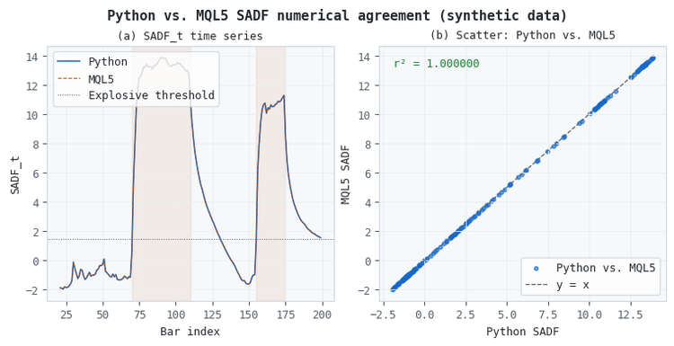
SADF computation cost: expanding vs. rolling window

Figure 2. 2-panel illustration of expanding vs. rolling window cost for SADF

Panel (a): Absolute inner-loop operation count for the expanding window (red, O(T²)) and the rolling window with L = 252 (green, O(L²) once T > L). The green line is flat beyond T = 252 because the lookback cap prevents further growth.
Panel (b): Ratio of expanding to rolling cost. At T = 1,000 bars the expanding window performs 15.4× more operations. At T = 5,000 bars (a 20-year daily series) that ratio reaches 394×. In a live EA running on every new bar, the rolling window is the only feasible implementation.

The rolling window changes the interpretation of SADF in one precise way: it answers "is the series explosive within the last L bars?" rather than "has it ever been explosive?". For a feature whose purpose is to select the current trading strategy — trend following when SADF is high, mean-reversion when SADF is low — the rolling interpretation is exactly correct. The relevant question is the current regime, not the historical peak. Only for long-run bubble monitoring, where detecting a multi-year accumulation requires the full expanding window, is the Python version with a bounded lookback (L = 504 or similar) more appropriate.

The SADF inner helper _SADFAtT() builds the diff and lagged-level arrays once for the window slice and runs the expanding start-point loop:

//+------------------------------------------------------------------+
//| _SADFAtT: compute supremum ADF statistic for one endpoint t_end  |
//|   within the rolling window [window_start, t_end].               |
//|   Returns the maximum ADF t-statistic over all start points.     |
//+------------------------------------------------------------------+
double CStructuralBreaks::_SADFAtT(int t_end, int window_start)
  {
   double bsadf = SB_EMPTY;
   //--- Build dp[] and lev[] once for this slice
   for(int j = 0; j < slice_len - 1; j++)
     {
      int k  = window_start + j;
      lev[j] = m_log_p[m_n - 1 - k];
      dp[j]  = m_log_p[m_n - 1 - (k+1)] - m_log_p[m_n - 1 - k];
     }
   //--- Inner start-point loop: OLS with intercept on each subsample
   for(int s = 0; s <= n_dp - tau; s++)
     {
      //--- Accumulate sums for intercept-augmented OLS
      double sx=0, sy=0, sxx=0, sxy=0;
      for(int i = s; i < s + tau; i++) { ... }
      //--- Compute t-statistic for beta (slope) with df = n-2
      if(t_val > bsadf) bsadf = t_val;
     }
   return(bsadf);
  }

The m_lookback parameter controls L. The default is 252 (one year of daily bars), appropriate for detecting swing and medium-term bubbles. For intraday bars at H1 frequency, 252 × 24 = 6,048 bars represents one year; setting lookback = 504 (two weeks of H1 bars) targets short-run explosive moves at that frequency.

Sub- and Super-Martingale Tests

The SM-Exp and SM-Power tests replace the ADF specification with direct regressions on functional forms of time, testing whether log-price follows an exponential or power-law trajectory. Both use the same rolling window convention as SADF:

//+------------------------------------------------------------------+
//| Sub-/Super-martingale test regressors:                           |
//|   SM-Exp: log(y_t) = log(α) + β·t + ξ_t   (t-stat on β)          |
//|   SM-Power: log(y_t) = log(α) + β·log(t) + ξ_t                   |
//+------------------------------------------------------------------+
double t_e = (double)(k - s);               // linear time index for SM-Exp
double t_p = (t_e > 0.0) ? MathLog(t_e) : 0.0;  // log-time index for SM-Power

Both report absolute-value t-statistics, so SMTExp(0) and SMTPower(0) are always non-negative where defined. A high SM-Exp value indicates that log-prices are following a linear time trend (exponential price growth); a high SM-Power value indicates power-law price growth. Including both alongside SADF gives the downstream model information about the functional form of the explosive trajectory, which is informative for sizing the bet and estimating the duration of the regime.

OLS Accumulation in Each Test Family

The three test families that require regression each implement their own inline OLS accumulation. The formulations differ because the Chow specification has no constant term, while the SADF and SMT specifications include an intercept.

The Chow DFC regression is Δyt = δ · yt−1 · Dt[τ*] + εt: no intercept. The slope estimator is β = ΣXY / ΣX², accumulated over the active segment only (k ≥ τ*). The residual variance is computed over the full sample, with df = n − 1 (one estimated parameter). The variance of the estimator is var(β) = σ² / ΣX². Using the intercept-adjusted beta formula (n·ΣXY − ΣX·ΣY) / (n·ΣX² − (ΣX)²) with no-intercept residuals produces a biased σ² and a deflated t-statistic; the residuals must be computed under the same model assumption as the estimator.

The SADF inner loop in _SADFAtT() regresses Δy on yt−1 with an intercept: y = α + β · x + ε. It accumulates the intercept-augmented normal equations — n·ΣXY − ΣX·ΣY in the numerator, n·ΣX² − (ΣX)² in the denominator — computes both α and β, and subtracts both from the residual in the second pass. The residual variance uses df = n − 2. The SMT start-point loop follows the same pattern, replacing the lagged level with a functional form of time (linear for SM-Exp, logarithmic for SM-Power).

In all three cases the inner loop allocates no temporary arrays beyond the pre-built slice. All sums accumulate in a single forward pass. The near-singular guard (|denom| < 1e-20) and the minimum valid-observation check (n ≥ 4) apply to every family. When either condition is met, the caller leaves the output array at SB_EMPTY rather than producing a NaN or crash. This is consistent with CMicrostructureFeatures.mqh: any feature value above SB_EMPTY + 1.0 is valid.

EA Integration and Feature Routing

The six structural break statistics output by CStructuralBreaks map onto two roles in an EA: regime detection and strategy selection. The CSW excess and SADF value determine which strategy is active; the Chow break-bar index conditions lookback windows; the SMT statistics sharpen the regime classification when the SADF signal is ambiguous.

#include <StructuralBreaks\CStructuralBreaks.mqh>

//+------------------------------------------------------------------+
//| Input parameters for structural break thresholds                 |
//+------------------------------------------------------------------+
input int    inp_lookback        = 252;
input int    inp_min_length      = 20;
input int    inp_n_bars          = 300;
input double inp_sadf_explosive  = 1.5;
input double inp_sadf_steady     = -0.5;

CStructuralBreaks *g_sb  = NULL;
datetime          g_last = -1;

//+------------------------------------------------------------------+
//| OnInit: create structural breaks engine                          |
//+------------------------------------------------------------------+
int OnInit()
  {
   g_sb = new CStructuralBreaks(_Symbol, _Period,
                                  inp_min_length, inp_lookback);
   if(g_sb == NULL) return(INIT_FAILED);
   return(INIT_SUCCEEDED);
  }

//+------------------------------------------------------------------+
//| OnTick: process new bar, read features, apply regime logic       |
//+------------------------------------------------------------------+
void OnTick()
  {
   //--- New bar check
   if(iTime(_Symbol, _Period, 0) == g_last) return;
   g_last = iTime(_Symbol, _Period, 0);

   //--- Compute statistics on the last inp_n_bars bars
   if(!g_sb.Calculate(1, inp_n_bars)) return;

   //--- Retrieve current SADF value (offset 0)
   double sadf = g_sb.SADFValue(0);
   if(sadf <= SB_EMPTY + 1.0) return;   // window not yet filled

   //--- Three-regime classifier based on SADF
   if(sadf > inp_sadf_explosive)
     {
      //--- Explosive regime: trend / event strategy
      //--- Refine with SMT for trajectory shape
      double smt_exp   = g_sb.SMTExp(0);
      double smt_power = g_sb.SMTPower(0);
      //--- smt_exp > smt_power → exponential acceleration likely
     }
   else if(sadf < inp_sadf_steady)
     {
      //--- Steady regime: mean-reversion strategy
      //--- half-life ≈ -log(2) / log(1 + beta) from ADF coefficient
     }
   else
     {
      //--- Unit-root zone: reduce exposure, wait
      //--- CSW excess confirms whether drift has accumulated
      double csw_excess = g_sb.CSWStat(0) - g_sb.CSWCritical(0);
     }
  }

The SADF thresholds inp_sadf_explosive and inp_sadf_steady are exposed as inputs rather than hard-coded. Their optimal values depend on the instrument, timeframe, and the lookback L; they should be set by examining the historical SADF distribution for the target symbol rather than assumed to be 1.5 and −0.5 universally. The validation script provides sample values at bar 0 that help calibrate these thresholds against live data before deployment.

StructuralBreaksViewer Indicator

The class described above is a computational engine with no visual output of its own. StructuralBreaksViewer.mq5 wraps it in a separate-window indicator that attaches to any chart and plots all six statistics simultaneously. Its primary purpose is calibration: examining the historical distribution of each statistic before committing to the threshold values used by the EA regime classifier.

Design

The indicator maintains six DRAW_LINE plot buffers, one per statistic. Each series can be enabled or disabled independently via boolean inputs (InpShowCSWStat, InpShowSADF, and so on). The CSW, Chow, SADF, and SMT families span different absolute ranges: the CSW statistic is typically bounded between 0 and 5; the SADF can range from −3 to 10 or beyond on trending instruments. Plotting all series on a single axis without adjustment produces an unreadable chart dominated by the largest values. The InpNormalize toggle addresses this by z-scoring each series independently over the visible window before writing to the plot buffer. The Comment() readout always displays the most recent raw value for each visible series, regardless of the normalize setting, so threshold calibration against the actual statistic scale is always available without restarting the indicator.

Computation runs once per new bar, not on every tick. The new-bar guard compares rates_total against the value stored on the previous call; a change triggers a full recompute of the most recent InpMaxBars bars. The O(L²) SADF and SMT kernels make this the dominant cost; on a daily chart with the default InpMaxBars = 400 and InpLookback = 252, a single call to Calculate() completes in well under one second. On intraday charts the same lookback covers far fewer calendar days; reducing InpLookback proportionally to the bar frequency keeps the computation within the same time budget.

//+------------------------------------------------------------------+
//| OnCalculate: indicator main loop – recompute on new bar only     |
//+------------------------------------------------------------------+
int OnCalculate(const int rates_total,
               const int prev_calculated,
               const int begin,
               const double &price[])
  {
   bool recompute = (prev_calculated == 0) || (rates_total != g_last_rt);
   if(recompute)
     {
      //--- ComputeFeatures populates g_raw and g_computed_n.
      //--- FillBuffers is called unconditionally: if compute fails,
      //--- g_computed_n is 0 and FillBuffers clears all buffers to
      //--- EMPTY_VALUE, preventing stale data from the previous pass.
      bool ok = ComputeFeatures(rates_total);
      FillBuffers(rates_total);
      if(ok) RefreshReadout();
      g_last_rt = rates_total;
     }
   return(rates_total);
  }

The FillBuffers() function separates the normalize decision from the compute step. When InpNormalize = true, it computes the mean and standard deviation of each series over all valid values in a single forward pass, then writes (v − mean) / sd to the plot buffer. When InpNormalize = false, it writes the raw value directly. In either case the Comment readout reads from g_latest[], which stores the most recent valid raw value populated by ComputeFeatures().

Known Limitations

Two structural limitations remain that would require a more significant architectural change to address.

The indicator computes all six statistics on every new bar regardless of which series are visible. When both InpShowSADF and the SMT inputs are false, the O(L²) kernels in _ComputeSADF() and _ComputeSMT() still run for all InpMaxBars bars. At InpMaxBars = 400 and InpLookback = 252, this dominates per-bar CPU time. Adding a compute-mask parameter to Calculate() would allow those kernels to be skipped entirely when the corresponding series are hidden, reducing per-bar cost by roughly 70% in CSW-only mode.

The indicator also recomputes all InpMaxBars statistics from scratch on every new bar. In reality, only the most recent endpoint changes; the prior n − 1 values are identical to what was computed on the previous bar. An incremental update would store the n − 1 prior SADF values and compute only the single new endpoint, reducing per-bar SADF cost from O(n · L²) to O(L²). This would make the indicator viable at higher bar counts without increasing the lookback cap.

Validation

The companion StructuralBreaksValidation.mq5 script checks five mathematical invariants that must hold on any valid symbol and timeframe:

Check	Property	Rationale
1	f.Count() == n_bars	Output arrays must match the requested bar count.
2	CSW critical ≥ √4.6 ≈ 2.14 everywhere defined	cα[n,t] = √(4.6 + log(span)) ≥ √4.6 for all spans ≥ 1.
3	SADF finite where defined	Any NaN or Inf indicates a residual variance or denominator fault.
4	SMT-Exp ≥ 0 where defined	SMT uses \|t-stat\|; absolute value is always non-negative.
5	Chow DFC finite where defined	Same residual-variance check as SADF.

Run the script on EURUSD D1 with the default 150-bar lookback before deploying any EA that uses CStructuralBreaks. If Check 2 fails, a negative best_span has been computed, indicating an index overflow in the inner CSW loop — verify that n_bars ≥ min_length + 4. If Check 3 or 5 fails, a near-zero variance case is producing a spurious Inf; lower min_length or increase n_bars to give the OLS estimator more data per window.

Python–MQL5 Numerical Agreement

The figure below verifies that the MQL5 SADF implementation reproduces the Python output to machine precision on the same 200-bar synthetic series used in Part 9 with two injected explosive episodes.

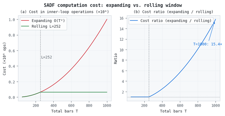
Python vs. MQL5 SADF numerical agreement (synthetic data)

Figure 3. 2-panel illustration of Python vs. MQL5 SADF agreement on 200 synthetic bars (two explosive episodes shaded)

Panel (a): SADF time series from both implementations overlaid. The Python (solid blue) and MQL5 (dashed orange) lines are visually identical. Both implementations correctly spike above the 1.5 explosive threshold during both injected episodes.
Panel (b): Scatter plot of Python vs. MQL5 output at each bar. The r² = 1.000000 confirms floating-point agreement. Any index convention error would shift points off the y = x diagonal by a systematic amount proportional to the series trend.

To reproduce this verification against your own data, export OHLCV bars from MetaTrader 5 as a CSV, run the Python get_sadf() from Part 9 on the log-price column, and compare bar-by-bar with the SADFValue() output from the script. Use the same min_length and lookback values in both; a mismatch in either parameter produces systematically different output that is easy to confuse with a formula error.

Conclusion

This article ported three structural break test families from Part 9 to MQL5 as a single include file, CStructuralBreaks.mqh, placed in MQL5/Include/StructuralBreaks/. The class provides six features per bar: CSW statistic and critical value, Chow DFC, SADF, SM-Exp, and SM-Power. Each test family implements its own inline OLS accumulation; Chow uses no-intercept OLS with df = n − 1, while SADF and SMT use intercept-augmented OLS with df = n − 2. All six statistics share the SB_EMPTY = −1e38 sentinel convention established in CMicrostructureFeatures.mqh.

The central design decision — rolling window rather than expanding window for SADF — bounds the per-bar computation to O(L²) rather than O(T²), making the implementation viable inside an EA on any realistic series length. The rolling window changes the interpretation of SADF from a historical maximum to a current-window maximum, which is the correct interpretation for a real-time regime-selection feature.

The index convention difference between Python (chronological) and MQL5 (time-series) is the dominant source of silent errors in porting work of this kind. Every compute method in the class works in chronological space internally and maps to time-series indices only at the output write step. This structure makes the statistical logic directly auditable against the chapter formulas.

The companion StructuralBreaksViewer.mq5 indicator wraps the class in a separate-window chart tool. Its z-score normalization toggle overlays the six statistics on a common axis for visual inspection; its raw-value Comment readout provides the actual statistic scale needed to calibrate the EA regime thresholds before deployment.

References

López de Prado, M. (2018). Advances in Financial Machine Learning. Wiley. Chapter 17.
Andrews, D. (1993). Tests for parameter instability and structural change with unknown change point. Econometrica, 61(4), 821–856.
Chow, G. (1960). Tests of equality between sets of coefficients in two linear regressions. Econometrica, 28(3), 591–605.
Homm, U., & Breitung, J. (2012). Testing for speculative bubbles in stock markets: A comparison of alternative methods. Journal of Financial Econometrics, 10(1), 198–231.
Phillips, P., Wu, Y., & Yu, J. (2011). Explosive behavior in the 1990s Nasdaq: When did exuberance escalate asset values?International Economic Review, 52, 201–226.
Phillips, P., & Yu, J. (2011). Dating the timeline of financial bubbles during the subprime crisis. Quantitative Economics, 2, 455–491.
Maddala, G., & Kim, I. (1998). Unit Roots, Cointegration and Structural Change. Cambridge University Press.
Greene, W. (2008). Econometric Analysis, 6th ed. Pearson Prentice Hall.

Attached Files

	File	Location	Description
1.	CStructuralBreaks.mqh	MQL5/Include/StructuralBreaks/	Structural break test engine. Provides six bar-indexed statistics: CSW statistic and critical value, Chow-Type DFC, SADF (rolling lookback L), SM-Exp, and SM-Power.
2.	StructuralBreaksViewer.mq5	MQL5/Indicators/StructuralBreaks/	Separate-window viewer indicator. Plots all six statistics with per-series visibility toggles and a z-score normalization toggle for threshold calibration.
3.	StructuralBreaksValidation.mq5	MQL5/Scripts/StructuralBreaks/	Validation script. Runs five invariant checks (count, CSW critical floor, SADF finiteness, SMT-Exp sign, Chow finiteness) and prints sample values at bar 0.

Attached files |

Download ZIP

MQL5.zip (13.59 KB)

Warning: All rights to these materials are reserved by MetaQuotes Ltd. Copying or reprinting of these materials in whole or in part is prohibited.

This article was written by a user of the site and reflects their personal views. MetaQuotes Ltd is not responsible for the accuracy of the information presented, nor for any consequences resulting from the use of the solutions, strategies or recommendations described.