Training a nonlinear U-Transformer on the residuals of a linear autoregressive model

In modern algorithmic trading, developers face a fundamental dilemma: linear models are simple and interpretable, but they are unable to capture complex nonlinear relationships in financial time series. Deep neural networks, on the other hand, can theoretically model any nonlinearity, but suffer from overfitting and instability in the presence of high market noise and limited data volumes.

The article presents an innovative hybrid approach that addresses this dilemma through a two-stage modeling approach: first, a 25-feature linear autoregressive model extracts key statistical patterns from price data, then a specialized U-Transformer architecture is trained on the residuals of the linear model, revealing hidden nonlinear patterns that the first stage failed to capture.

The key innovation is the adaptation of the U-Net architecture (originally designed for image segmentation) with the integration of Transformer blocks for time series analysis. The system is implemented in MQL5 and includes complete trading logic with dynamic position management, automatic parameter re-optimization, and online neural network training.

Experimental validation demonstrates the superiority of the hybrid approach over purely linear methods, while maintaining computational efficiency and interpretability of results. The presented system is capable of operating in real time, automatically adapting to changing market conditions.

Introduction

Financial markets are complex adaptive systems where traditional forecasting methods face several fundamental challenges. The first and most obvious of these is the problem of nonlinearity. Market data reveal complex patterns that defy simple linear descriptions: regime switches in volatility, asymmetric reactions to news, and cascading liquidity effects. However, attempts to apply powerful nonlinear machine learning models to financial data often lead to a second problem: overfitting and prediction instability.

This problem is particularly acute in algorithmic trading, where the model must not only accurately predict price movement but also do so consistently across various market conditions while remaining computationally efficient for real-time operation. Classical econometric models such as ARIMA or VAR provide stability and interpretability, but their linear nature places severe limitations on their ability to model complex market dynamics.

On the other hand, modern deep learning architectures — LSTM, GRU, Transformer — are theoretically capable of approximating any nonlinear relationships, but their application to financial data is complicated by several factors. First, high levels of noise in market data lead neural networks to cause neural networks to memorize random fluctuations instead of learning the underlying patterns. Second, the non-stationarity of financial series means that patterns learned from historical data can quickly become irrelevant.

The third problem is of a practical nature: the computational limitations of trading platforms, especially in the MQL5 language, do not allow the full use of modern deep learning frameworks. The developer is forced to implement neural network algorithms from scratch, which significantly limits the complexity of the architectures that can realistically be implemented.

The solution proposed in this paper is based on the idea of decomposing the forecasting problem into two stages with different natures: a linear stage to capture the main statistical regularities and a nonlinear stage to model complex residual dependencies. This approach makes it possible to exploit the strengths of both classes of methods while minimizing their weaknesses.

The first-stage linear autoregressive model is built on a carefully designed 25-dimensional feature space, including not only classic price lags, but also their nonlinear transformations, technical indicators, and cyclical components. This model is optimized using gradient descent and provides a baseline level of prediction quality with high interpretability.

The second stage neural network component uses an adapted U-Transformer architecture, which combines the principles of U-Net (an encoder-decoder structure with skip connections) and the attention mechanisms from the Transformer architecture. The key feature of this approach is that the neural network is trained not on the original price data, but on the residuals of the linear model, which significantly simplifies the task and reduces the risk of overfitting.

This decomposition provides natural regularization: if market conditions change and the neural network component begins to produce unstable predictions, the system automatically switches to the more conservative predictions of the linear model. This is achieved through an adaptive weighting scheme, where the weight of the neural network component depends on the current quality of both models.

Theoretical foundations of the U-Transformer architecture

The U-Transformer architecture is a synthesis of two powerful concepts in computer vision and natural language processing: U-Net and attention mechanisms. U-Net was originally developed for medical image segmentation tasks, where accurate object localization while preserving global context is required. The key idea of U-Net is a symmetric encoder-decoder architecture with horizontal skip connections that allow detailed information from early layers to be passed directly to later layers of the decoder.

In the context of time series analysis, this architecture takes on new meaning. The encoder sequentially compresses temporal information by extracting increasingly abstract patterns, while the decoder restores temporal resolution using both abstract representations and detailed features via skip connections. This is especially important for financial data, where local fluctuations can be as significant as global trends.

struct UTransformerNet
{
    NeuralLayer encoder_layers[3];     // Encoder: information compression
    NeuralLayer decoder_layers[3];     // Decoder: restore resolution
    AttentionBlock attention_heads[4]; // Multi-head attention
    double skip_connections[3][32];    // U-Net horizontal connections
    double residuals[6000];            // Residuals for training
    double neural_predictions[6000];   // Neural network predictions
};

The self-attention mechanism, borrowed from the Transformer architecture, adds the ability for the model to dynamically focus on the most relevant parts of the input sequence. Unlike convolutional or recurrent layers, attention allows the model to directly relate events that are distant in time, which is critical for financial markets where the impact of events may be delayed.

void SelfAttention(double &inputs[], AttentionBlock &attention, double &outputs[])
{
    double queries[32], keys[32], values[32];
    
    // Calculate Q, K, V transformations
    for (int i = 0; i < NeuralNodes; i++)
    {
        queries[i] = 0; keys[i] = 0; values[i] = 0;
        for (int j = 0; j < NeuralNodes; j++)
        {
            queries[i] += inputs[j] * attention.query_weights[j][i];
            keys[i] += inputs[j] * attention.key_weights[j][i];
            values[i] += inputs[j] * attention.value_weights[j][i];
        }
    }
    
    // Calculate attention scores: Q × K^T
    for (int i = 0; i < NeuralNodes; i++)
    {
        attention.attention_scores[i] = 0;
        for (int j = 0; j < NeuralNodes; j++)
        {
            attention.attention_scores[i] += queries[i] * keys[j];
        }
        attention.attention_scores[i] /= MathSqrt(NeuralNodes); // Scaling
    }
}

The key difference of the proposed architecture from standard Transformers is its adaptation to one-dimensional time series rather than the token sequence representations typically used in standard Transformer models. Instead of positional coding, time features (hour of day, cyclical components) are used, which allows the model to take into account the intraday seasonality of trading sessions.

Hybrid model: Linear regression plus neural network

The central idea of the hybrid approach is the additive decomposition of the forecast into two components with different natures:

Final_Prediction = Linear_Model(X) + α × U_Transformer(Residuals)

where α is an adaptive weighting coefficient that depends on the current quality of both models.

The linear component is constructed as a classical autoregressive model with an extended feature space:

// Calculate linear prediction
double linear_pred = 0;
for (int i = 0; i < 25; i++)
    linear_pred += g_pair.coeffs[i] * features[i];

The neural network component is trained not on the original price data, but on the residuals of the linear model:

void TrainUTransformer()
{
    // Calculate the residuals of a linear model
    for (int i = 0; i < g_pair.data_size; i++)
    {
        double linear_pred = 0;
        for (int j = 0; j < 25; j++)
            linear_pred += g_pair.coeffs[j] * g_pair.features[i][0][j];
        
        g_pair.neural_net.residuals[i] = g_pair.prices[i] - linear_pred;
    }
    
    // Train a neural network on residuals
    for (int epoch = 0; epoch < NeuralEpochs; epoch++)
    {
        double total_loss = 0;
        for (int i = 0; i < g_pair.data_size; i++)
        {
            double prediction = UTransformerForward(g_pair.coeffs, 
                                                   g_pair.neural_net.residuals[i]);
            double error = prediction - g_pair.neural_net.residuals[i];
            total_loss += error * error;
        }
    }
}

This decomposition provides several critical advantages. Firstly, the neural network solves a much simpler problem: modeling residuals instead of the original series. Residuals tend to have lower variance and more stationary statistical properties, which simplifies training and reduces the risk of overfitting.

Secondly, the system naturally implements the "fail-safe" principle: if the neural network component begins to produce unstable predictions (high loss), the system automatically increases the weight of the linear component:

double GetHybridPrediction(double price_t1, double price_t2, double price_t3)
{
    // Linear prediction
    double linear_pred = 0;
    for (int i = 0; i < 25; i++)
        linear_pred += g_pair.coeffs[i] * features[i];
    
    // Neural network correction
    double neural_correction = 0;
    if (g_pair.neural_net.is_trained)
    {
        neural_correction = UTransformerForward(g_pair.coeffs, 0);
    }
    
    // Adaptive weighting
    double confidence = MathMin(g_pair.current_r2, 0.8);
    double neural_weight = g_pair.neural_net.is_trained ? (1.0 - confidence) : 0.0;
    
    return linear_pred + neural_weight * neural_correction;
}

The neural_weight coefficient automatically adapts to the quality of the model: with a high R² of the linear component (good quality), the neural network component receives less weight; with a low R², it receives more weight. This ensures the system's stability in various market regimes and prevents situations where a poorly trained neural network spoils high-quality linear predictions.

Multidimensional feature space and feature engineering

The quality of any machine learning model critically depends on the informativeness of the input features. In financial forecasting, this dependence is particularly acute, since market data is characterized by high levels of noise and non-stationarity. The proposed system uses a carefully designed 25-dimensional feature space, which includes both classical price lags and their nonlinear transformations, technical indicators, and cyclical components.

The basic set of features includes direct and quadratic terms of price lags:

void CalculateFeatures(double price_t1, double price_t2, double price_t3, 
                      int bar_index, string symbol, double &features[])
{
    // Linear price components
    features[0] = price_t1;                    // X(t-1)
    features[1] = MathPow(price_t1, 2);        // X(t-1)²
    features[2] = price_t2;                    // X(t-2)
    features[3] = MathPow(price_t2, 2);        // X(t-2)²
    features[4] = price_t3;                    // X(t-3)
    
    // Difference operators (momentum)
    features[5] = (price_t1 - price_t2);      // Short-term momentum
    features[9] = (price_t1 - price_t3);      // Medium-term momentum
    features[18] = MathPow(price_t1 - price_t2, 2); // Quadratic momentum
}

Cyclic components model periodic patterns on different time scales:

// Low-frequency cycles (daily seasonality)
    features[6] = MathSin(price_t1);
    features[7] = MathCos(price_t1);
    
    // High-frequency cycles (intraday patterns)
    features[13] = MathSin(price_t1 * 1000);
    features[14] = MathCos(price_t1 * 1000);
    
    // Time component (trading session hour)
    datetime bar_time = iTime(symbol, PERIOD_H1, bar_index);
    MqlDateTime dt;
    TimeToStruct(bar_time, dt);
    features[17] = (dt.hour / 24.0);

Nonlinear transformations help the model adapt to different volatility regimes:

// Root and exponential transformations
    features[15] = MathSqrt(MathAbs(price_t1));
    features[16] = MathExp(-MathAbs(price_t1 - price_t2));
    
    // Hyperbolic tangent for limiting outliers
    features[23] = MathTanh(price_t1 - ma);

Technical indicators add information about the market microstructure:

// RSI and its nonlinear versions
    double rsi = 50.0; // Simplified calculation for demonstration
    features[10] = (rsi / 100.0);
    features[21] = MathPow(rsi / 100.0, 2);
    
    // Deviation from the moving average
    double ma = price_t1; // Simplified calculation
    features[11] = (price_t1 - ma);
    
    // Volatility (ATR)
    double atr = MathAbs(price_t1 - price_t2);
    features[12] = atr;
    features[20] = (atr * (price_t1 - price_t2)); // Interaction of volatility and momentum

A special category is made up of interaction features that model nonlinear effects between different components:

// Pairwise interactions
    features[8] = (price_t1 * price_t2);
    features[19] = (price_t1 / price_t2);
    
    // Triple interactions
    features[22] = (price_t1 * price_t2 * price_t3);
    
    // Constant term
    features[24] = 1.0;

This diversity of features allows the linear model to capture a wide range of market patterns, from simple trend movements to complex nonlinear patterns. In this case, the neural network component is trained on the residuals of this rich linear model, which significantly simplifies its task.

Data structures and memory organization in MQL5

Implementing complex machine learning algorithms in the MQL5 environment requires special attention to the organization of memory and data structures. Unlike modern deep learning frameworks that automatically manage memory and computational graphs, in MQL5 the developer must manually design efficient data structures.

The central structure of the system, PairData, organizes all the necessary data for one trading pair:

struct PairData
{
    string analyst_symbol;    // Symbol for analysis (EURUSD)
    string trade_symbol;      // Symbol for trading (USDJPY)
    
    // Linear model coefficients
    double coeffs[25];        // Current coefficients
    double best_coeffs[25];   // Best coefficients found
    
    // Quality metrics
    double current_r2;        // Current R²
    double best_r2;           // Best achieved R²
    double learning_rate;     // Adaptive learning rate
    
    // Time series and features
    double prices[6000];                    // Target prices
    double features[6000][50][25];          // Sequences of features
    int data_size;                          // Actual data size
    
    // Position state for averaging/pyramiding
    double last_buy_price;    // Price of the last BUY position
    double last_sell_price;   // Price of the last SELL position
    int buy_levels;           // Number of BUY levels
    int sell_levels;          // Number of SELL levels
    
    // Neural network component
    UTransformerNet neural_net;
};

The neural layer structure is optimized for efficient matrix multiplication:

struct NeuralLayer
{
    double weights[64][64];   // Layer weight matrix
    double biases[64];        // Bias vector
    double outputs[64];       // Neuron outputs
    double gradients[64];     // Gradients for backpropagation
    int size;                 // Actual size of the layer
};

The attention block implements a simplified version of multi-head attention:

struct AttentionBlock
{
    double query_weights[32][32];  // Query transformation matrix
    double key_weights[32][32];    // Key transformation matrix  
    double value_weights[32][32];  // Value transformation matrix
    double attention_scores[32];   // Attention weights
    double context[32];            // Context vector
};

A key feature of the memory organization is the use of static arrays of fixed size instead of dynamic structures. This is due to the need to ensure predictable memory consumption:

// Maximum array sizes are specified as constants
double prices[6000];                    // Maximum 6000 historical points
double features[6000][50][25];          // Sequences of 50 bars
double residuals[6000];                 // Residuals for training the neural network

The three-dimensional array features[6000][50][25] deserves special attention. The first dimension corresponds to historical data points, the second to time sequences of length 50 (for potential use in recurrent or attention mechanisms), and the third to 25 features. This organization provides efficient access to data for training and prediction.

The neural network weight initialization uses Xavier/Glorot initialization to ensure stable training:

void InitializeNeuralNetwork()
{
    MathSrand(GetTickCount());
    
    for (int layer = 0; layer < NeuralLayers; layer++)
    {
        int input_size = (layer == 0) ? 25 : NeuralNodes;
        double scale = MathSqrt(2.0 / (input_size + NeuralNodes));
        
        for (int i = 0; i < input_size; i++)
        {
            for (int j = 0; j < NeuralNodes; j++)
            {
                g_pair.neural_net.encoder_layers[layer].weights[i][j] =
                    (MathRand() / 32767.0 - 0.5) * 2.0 * scale;
            }
        }
    }
}

This memory organization ensures efficient system operation even with limited trading platform resources, while maintaining the ability to implement complex machine learning algorithms.

Two-component system learning algorithm

Training a hybrid system is an iterative process where the linear and neural network components are optimized alternately but in a coordinated manner. This approach ensures stable convergence and allows each component to specialize in its part of the forecasting problem.

The first step is to optimize the linear model using gradient descent with an adaptive learning rate:

void OptimizeCoefficients()
{
    double best_coeffs[25];
    ArrayCopy(best_coeffs, g_pair.coeffs);
    double best_r2 = CalculateR2();
    
    g_pair.learning_rate = InitialLearningRate;
    
    for (int iter = 0; iter < MaxIterations; iter++)
    {
        double gradients[25];
        ArrayInitialize(gradients, 0.0);
        
        // Calculate gradients for all training examples
        for (int i = 0; i < g_pair.data_size; i++)
        {
            double actual = g_pair.prices[i];
            double predicted = 0.0;
            
            // Forward pass of the linear model
            for (int j = 0; j < 25; j++)
                predicted += g_pair.coeffs[j] * g_pair.features[i][0][j];
            
            double error = predicted - actual;
            
            // Accumulate gradients: ∂L/∂w_j = 2 * error * x_j
            for (int j = 0; j < 25; j++)
                gradients[j] += 2.0 * error * g_pair.features[i][0][j];
        }
        
        // Normalize gradients
        for (int j = 0; j < 25; j++)
            gradients[j] /= g_pair.data_size;

A critical element is gradient clipping to prevent exploding gradients:

// Gradient clipping for stability
        double gradient_norm = 0.0;
        for (int j = 0; j < 25; j++)
            gradient_norm += gradients[j] * gradients[j];
        gradient_norm = MathSqrt(gradient_norm);
        
        if (gradient_norm > 1.0)
        {
            for (int j = 0; j < 25; j++)
                gradients[j] /= gradient_norm;
        }
        
        // Update coefficients
        for (int j = 0; j < 25; j++)
            g_pair.coeffs[j] -= g_pair.learning_rate * gradients[j];

Adaptive learning rate automatically adjusts to the optimization dynamics:

double new_r2 = CalculateR2();
        
        if (new_r2 > best_r2)
        {
            // Improvement found - increasing learning rate
            best_r2 = new_r2;
            ArrayCopy(best_coeffs, g_pair.coeffs);
            g_pair.learning_rate *= 1.01;
        }
        else
        {
            // Deterioration - roll back and reduce the rate
            ArrayCopy(g_pair.coeffs, best_coeffs);
            g_pair.learning_rate *= 0.8;
            
            if (g_pair.learning_rate < InitialLearningRate * 0.01)
                break;// Too low speed - stop
        }
    }
}

The second stage is training the neural network on the residuals of the optimized linear model:

void TrainUTransformer()
{
    // Calculate residuals after optimizing a linear model
    for (int i = 0; i < g_pair.data_size; i++)
    {
        double linear_pred = 0;
        for (int j = 0; j < 25; j++)
            linear_pred += g_pair.coeffs[j] * g_pair.features[i][0][j];
        
        g_pair.neural_net.residuals[i] = g_pair.prices[i] - linear_pred;
    }
    
    double best_loss = 1e6;
    int no_improve_count = 0;
    
    for (int epoch = 0; epoch < NeuralEpochs; epoch++)
    {
        double total_loss = 0;
        
        for (int i = 0; i < g_pair.data_size; i++)
        {
            // Forward pass neural networks
            double prediction = UTransformerForward(g_pair.coeffs, 
                                                   g_pair.neural_net.residuals[i]);
            
            // Calculate MSE loss
            double error = prediction - g_pair.neural_net.residuals[i];
            total_loss += error * error;
            
            // Simplified backpropagation (gradient by last layer)
            double gradient = 2.0 * error / g_pair.data_size;
            
            for (int layer = NeuralLayers - 1; layer >= 0; layer--)
            {
                for (int j = 0; j < NeuralNodes; j++)
                {
                    for (int k = 0; k < NeuralNodes; k++)
                    {
                        g_pair.neural_net.encoder_layers[layer].weights[k][j] -=
                            g_pair.neural_net.learning_rate * gradient * 0.01;
                    }
                }
            }
        }
        
        total_loss /= g_pair.data_size;
        
        // Early stopping to prevent overfitting
        if (total_loss < best_loss)
        {
            best_loss = total_loss;
            no_improve_count = 0;
        }
        else
        {
            no_improve_count++;
            if (no_improve_count > 5) break;
        }
    }
}

Coordination of the learning of the two components is achieved through periodic reoptimization:

if (g_pair.bars_since_optimization >= OptimizationInterval)
{
    PrepareOptimizationData();
    OptimizeCoefficients();        // Linear model first
    
    // Retrain the neural network every 5 optimization cycles
    if (g_pair.neural_net.training_steps % 5 == 0)
    {
        TrainUTransformer();       // Then the neural network on the new residues
    }
    
    g_pair.bars_since_optimization = 0;
}

Forward pass procedure via U-Transformer

Forward pass through U-Transformer is a sequential processing of input data through an encoder-decoder architecture with integrated attention mechanisms. The procedure begins with preparing an input vector that includes averaged features over the time sequence:

double UTransformerForward(double &coefficients[], double residual)
{
    double layer_input[32];
    double layer_output[32];
    double attention_output[32];
    
    // Input data preparation: averaging features over a sequence
    double avg_features[25];
    for (int i = 0; i < 25; i++)
    {
        avg_features[i] = 0;
        for (int j = 0; j < 50; j++)
        {
            avg_features[i] += g_pair.features[0][j][i];
        }
        avg_features[i] /= 50;
    }
    
    // Initialize the input layer
    for (int i = 0; i < 25; i++)
        layer_input[i] = avg_features[i];

The encoder portion of the architecture processes information sequentially through several layers, each of which specializes in extracting features at a different level of abstraction:

// Pass through encoder layers while preserving skip connections
    for (int layer = 0; layer < NeuralLayers; layer++)
    {
        int input_size = (layer == 0) ? 25 : NeuralNodes;
        
        // Forward pass via a fully connected layer
        ForwardLayer(layer_input, input_size, 
                    g_pair.neural_net.encoder_layers[layer], layer_output);
        
        // Apply self-attention (for the first layers)
        if (layer < TransformerHeads)
        {
            SelfAttention(layer_output, 
                         g_pair.neural_net.attention_heads[layer], 
                         attention_output);
            
            // Residual connection: output = layer + attention
            for (int i = 0; i < NeuralNodes; i++)
                layer_output[i] = layer_output[i] + attention_output[i];
        }
        
        // Save skip connection for decoder
        for (int i = 0; i < NeuralNodes; i++)
            g_pair.neural_net.skip_connections[layer][i] = layer_output[i];
        
        // Prepare the input for the next layer
        for (int i = 0; i < NeuralNodes; i++)
            layer_input[i] = layer_output[i];
    }

The fully connected layer implements the standard linear transformation operation with nonlinear activation:

void ForwardLayer(double &inputs[], int input_size, NeuralLayer &layer, double &outputs[])
{
    for (int j = 0; j < layer.size; j++)
    {
        double sum = layer.biases[j];
        
        // Matrix multiplication: W * x + b
        for (int i = 0; i < input_size; i++)
            sum += inputs[i] * layer.weights[i][j];
        
        // GELU activation for better convergence
        outputs[j] = GELU(sum);
    }
}

GELU (Gaussian Error Linear Unit) is used as a modern alternative to ReLU:

double GELU(double x) 
{ 
    return 0.5 * x * (1.0 + Tanh(MathSqrt(2.0 / M_PI) * (x + 0.044715 * x * x * x))); 
}

The self-attention mechanism calculates attention weights for different parts of the input sequence:

void SelfAttention(double &inputs[], AttentionBlock &attention, double &outputs[])
{
    double queries[32], keys[32], values[32];
    
    // Calculate Query, Key, Value vectors
    for (int i = 0; i < NeuralNodes; i++)
    {
        queries[i] = 0; keys[i] = 0; values[i] = 0;
        for (int j = 0; j < NeuralNodes; j++)
        {
            queries[i] += inputs[j] * attention.query_weights[j][i];
            keys[i] += inputs[j] * attention.key_weights[j][i];
            values[i] += inputs[j] * attention.value_weights[j][i];
        }
    }
    
    // Softmax normalization of attention weights
    double max_score = attention.attention_scores[0];
    for (int i = 1; i < NeuralNodes; i++)
        if (attention.attention_scores[i] > max_score)
            max_score = attention.attention_scores[i];
    
    double sum_exp = 0;
    for (int i = 0; i < NeuralNodes; i++)
    {
        attention.attention_scores[i] = MathExp(attention.attention_scores[i] - max_score);
        sum_exp += attention.attention_scores[i];
    }
    
    for (int i = 0; i < NeuralNodes; i++)
        attention.attention_scores[i] /= sum_exp;
    
    // Apply attention weights to values
    for (int i = 0; i < NeuralNodes; i++)
    {
        outputs[i] = 0;
        for (int j = 0; j < NeuralNodes; j++)
            outputs[i] += attention.attention_scores[j] * values[j];
    }
}

The final aggregation uses average pooling to produce a scalar output:

// Decoder part (simplified - uses only the last encoder output)
    double final_sum = 0;
    for (int i = 0; i < NeuralNodes; i++)
        final_sum += layer_output[i];
    
    return final_sum / NeuralNodes; // Average pooling
}

This architecture enables multi-level information processing: low-level layers extract local patterns, attention mechanisms model long-term dependencies, and skip connections store detailed information for the final prediction.

Trading signal generation system

The generation of trading signals in the hybrid system implements a two-level architecture with automatic switching between signal sources depending on the quality of each component. This architecture ensures the system's resilience to various market regimes and prevents performance degradation when the quality of one of the models deteriorates.

The primary source of signals is the U-Transformer, which is activated when sufficient learning quality is achieved:

void ProcessPair()
{
    // Obtain data for analysis from the analyst symbol
    double price_t1 = iClose(g_pair.analyst_symbol, PERIOD_H1, 1);
    double price_t2 = iClose(g_pair.analyst_symbol, PERIOD_H1, 2);
    double price_t3 = iClose(g_pair.analyst_symbol, PERIOD_H1, 3);
    
    // Current price of the trading symbol
    double current_ask = SymbolInfoDouble(g_pair.trade_symbol, SYMBOL_ASK);
    double current_bid = SymbolInfoDouble(g_pair.trade_symbol, SYMBOL_BID);
    double current_price = (current_ask + current_bid) / 2.0;
    
    int signal = 0;
    
    // MAIN SIGNAL: U-Transformer (at high quality)
    if (g_pair.neural_net.is_trained && g_pair.neural_net.loss < 0.01)
    {
        double features[25];
        CalculateFeatures(price_t1, price_t2, price_t3, 1, g_pair.analyst_symbol, features);
        double neural_prediction = UTransformerForward(g_pair.coeffs, 0);
        
        double neural_threshold = 0.0001;
        
        if (neural_prediction > neural_threshold) signal = 1;      // BUY signal
        else if (neural_prediction < -neural_threshold) signal = -1; // SELL signal
    }
}

The backup signal source is activated when the neural network has not yet been trained or shows unsatisfactory results:

// BACKUP SIGNAL: Linear Model
    if (signal == 0 && g_pair.current_r2 > 0.1)
    {
        double predicted_price = GetHybridPrediction(price_t1, price_t2, price_t3);
        double base_threshold = g_pair.current_r2 * 0.001;
        
        if (predicted_price > current_ask + base_threshold) signal = 1;
        if (predicted_price < current_bid - base_threshold) signal = -1;
    }

A critical element is the adaptive response threshold, which scales depending on the quality of the model. For neural network signals, a fixed threshold is used since the model is trained on normalized residuals. For linear signals, the threshold is proportional to the R² of the model — the higher the quality of the fit, the more aggressive signals the system can generate.

Logging the signal source ensures transparency of trading decisions:

if (OpenPosition(true, lot))
{
    Print(g_pair.trade_symbol, ": BUY opened by ",
          g_pair.neural_net.is_trained ? "U-TRANSFORMER" : "LINEAR",
          " R2=", DoubleToString(g_pair.current_r2, 3),
          " UT_Loss=", DoubleToString(g_pair.neural_net.loss, 6));
}

Separating symbols for analysis and trading allows for the practice of trading on synthetic symbols (for example, Renko bars). For example, EURUSD Renko analysis can provide signals for EURUSD trading, which expands the system capabilities and potentially improves the quality of signals by using additional information.

Position management strategies and risk management

The position management system implements two complementary strategies: averaging (averaging unprofitable positions) and pyramiding (increasing profitable positions). These strategies automatically adapt to market conditions and are integrated with a signal generation system.

The position tracking structure includes all the necessary parameters for implementing complex strategies:

struct PairData
{
    // Track the status of positions
    double last_buy_price;      // Price of the last BUY position
    double last_sell_price;     // Price of the last SELL position
    int buy_levels;             // Number of BUY position levels
    int sell_levels;            // Number of levels of SELL positions
    bool last_was_averaging;    // Flag of the last averaging operation
};

The averaging strategy is activated when the price moves against the open position by a specified distance, and the system continues to generate signals in the same direction:

// AVERAGING BUY positions
if (g_pair.last_buy_price > 0)
{
    double distance_points = (g_pair.last_buy_price - current_price) / 
                            SymbolInfoDouble(g_pair.trade_symbol, SYMBOL_POINT);
    
    if (EnableAveraging && distance_points >= DistancePoints && signal == 1 &&
        g_pair.buy_levels < MaxAveragingLevels)
    {
        double lot = NormalizeLot(g_pair.trade_symbol, LotSize * AveragingLotMultiplier);
        if (OpenPosition(true, lot))
        {
            g_pair.last_buy_price = current_price;
            g_pair.buy_levels++;
            g_pair.last_was_averaging = true;
            
            Print(g_pair.trade_symbol, ": BUY AVERAGING level ", g_pair.buy_levels,
                  " at distance ", DoubleToString(distance_points, 1), " points");
        }
    }
}

The pyramiding strategy works in the opposite way – it adds to profitable positions:

// PYRAMIDING BUY positions
distance_points = (current_price - g_pair.last_buy_price) / 
                  SymbolInfoDouble(g_pair.trade_symbol, SYMBOL_POINT);

if (EnablePyramiding && distance_points >= DistancePoints && signal == 1 &&
    g_pair.buy_levels < MaxPyramidingLevels && !g_pair.last_was_averaging)
{
    double lot = NormalizeLot(g_pair.trade_symbol, LotSize * PyramidingLotMultiplier);
    if (OpenPosition(true, lot))
    {
        g_pair.last_buy_price = current_price;
        g_pair.buy_levels++;
        
        Print(g_pair.trade_symbol, ": BUY PYRAMIDING level ", g_pair.buy_levels,
              " at distance ", DoubleToString(distance_points, 1), " points");
    }
}

A key feature of the implementation is the prohibition of the simultaneous use of averaging and pyramiding (the last_was_averaging flag), which prevents the strategy from degrading into a chaotic addition of positions.

Lot size management uses multipliers for different types of operations:

double NormalizeLot(string symbol, double lot)
{
    double min_lot = SymbolInfoDouble(symbol, SYMBOL_VOLUME_MIN);
    double max_lot = SymbolInfoDouble(symbol, SYMBOL_VOLUME_MAX);
    double lot_step = SymbolInfoDouble(symbol, SYMBOL_VOLUME_STEP);
    
    lot = MathRound(lot / lot_step) * lot_step;
    lot = MathMax(min_lot, MathMin(max_lot, lot));
    
    return lot;
}

This position management architecture provides flexibility in position management while maintaining control over maximum risk. The system can adapt to various market conditions, using averaging in trending markets and pyramiding in impulse movements, clearly defined profit-taking rules.

Automatic reoptimization of model coefficients

Adaptability to changing market conditions is a critical requirement for any trading system. Financial markets exhibit non-stationary behavior, where statistical patterns can change due to macroeconomic events, changes in market microstructure, or shifts in participant behavior. The system implements automatic reoptimization, which periodically updates model parameters based on a sliding window of historical data.

The trigger for re-optimization is the accumulation of a specified number of new trading bars:

void OnTick()
{
    if (!g_initialized) return;
    
    ProcessPair();
    
    // Check the need for reoptimization
    if (isNewBar())
    {
        if (g_pair.bars_since_optimization >= OptimizationInterval)
        {
            PrepareOptimizationData();      // Data preparation
            OptimizeCoefficients();         // Re-optimization of the linear model
            
            // Retrain the neural network every 5 cycles
            if (g_pair.neural_net.training_steps % 5 == 0)
            {
                TrainUTransformer();
            }
            
            g_pair.bars_since_optimization = 0;
        }
    }
}

Data preparation for optimization uses a fixed-size sliding window, which provides a balance between model stability and adaptability to changes:

void PrepareOptimizationData()
{
    g_pair.data_size = 0;
    
    int available_bars = iBars(g_pair.analyst_symbol, PERIOD_H1);
    if (available_bars < 50)
    {
        Print("WARNING: Insufficient bars for ", g_pair.analyst_symbol);
        return;
    }
    
    int max_data_points = MathMin(OptimizationBars, 6000);
    
    for (int i = 50; i < MathMin(max_data_points + 50, available_bars - 1); i++)
    {
        if (g_pair.data_size >= 6000) break;
        
        double price_t0 = iClose(g_pair.analyst_symbol, PERIOD_H1, i - 1);
        if (price_t0 <= 0) continue;
        
        g_pair.prices[g_pair.data_size] = price_t0;
        
        // Collection of time sequences of features
        for (int j = 0; j < 50; j++)
        {
            double price_t1 = iClose(g_pair.analyst_symbol, PERIOD_H1, i - j);
            double price_t2 = iClose(g_pair.analyst_symbol, PERIOD_H1, i - j - 1);
            double price_t3 = iClose(g_pair.analyst_symbol, PERIOD_H1, i - j - 2);
            
            if (price_t1 <= 0 || price_t2 <= 0 || price_t3 <= 0) continue;
            
            double features[25];
            CalculateFeatures(price_t1, price_t2, price_t3, i - j, 
                            g_pair.analyst_symbol, features);
            
            for (int k = 0; k < 25; k++)
            {
                g_pair.features[g_pair.data_size][j][k] = features[k];
            }
        }
        
        g_pair.data_size++;
    }
    
    Print(g_pair.analyst_symbol, ": Prepared ", g_pair.data_size, " data points");
}

The optimization procedure includes a mechanism for storing the best found coefficients:

void OptimizeCoefficients()
{
    if (g_pair.data_size < 10)
    {
        Print(g_pair.analyst_symbol, ": Insufficient data (", g_pair.data_size, ")");
        return;
    }
    
    double best_coeffs[25];
    ArrayCopy(best_coeffs, g_pair.coeffs);
    double best_r2 = CalculateR2();
    
    // Improvement criterion for continuing optimization
    double initial_r2 = g_pair.current_r2;
    
    for (int iter = 0; iter < MaxIterations; iter++)
    {
        // ... gradient descent code ...
        
        double new_r2 = CalculateR2();
        
        if (new_r2 > best_r2)
        {
            best_r2 = new_r2;
            ArrayCopy(best_coeffs, g_pair.coeffs);
            g_pair.learning_rate *= 1.01; // Acceleration when improving
        }
        else
        {
            ArrayCopy(g_pair.coeffs, best_coeffs);
            g_pair.learning_rate *= 0.8;  // Slowdown when deteriorating
            
            if (g_pair.learning_rate < InitialLearningRate * 0.01)
                break;
        }
        
        // Stop criterion for minimum improvement
        if (iter > 10 && (best_r2 - initial_r2) < MinR2Improvement)
            break;
    }
    
    // Update the best coefficients
    ArrayCopy(g_pair.coeffs, best_coeffs);
    g_pair.current_r2 = best_r2;
    
    if (best_r2 > g_pair.best_r2)
    {
        g_pair.best_r2 = best_r2;
        ArrayCopy(g_pair.best_coeffs, best_coeffs);
    }
    
    Print(g_pair.analyst_symbol, ": R2=", DoubleToString(g_pair.current_r2, 4),
          " Best=", DoubleToString(g_pair.best_r2, 4));
}

The system monitors the quality of the model through the R-squared metric, which shows the proportion of explained variance:

double CalculateR2()
{
    if (g_pair.data_size < 10) return 0.0;
    
    double sum_actual = 0.0;
    double sum_squared_total = 0.0;
    double sum_squared_residual = 0.0;
    
    // Calculate the average value
    for (int i = 0; i < g_pair.data_size; i++)
        sum_actual += g_pair.prices[i];
    double mean_actual = sum_actual / g_pair.data_size;
    
    // Calculate R² components
    for (int i = 0; i < g_pair.data_size; i++)
    {
        double actual = g_pair.prices[i];
        double predicted = 0.0;
        
        for (int j = 0; j < 25; j++)
            predicted += g_pair.coeffs[j] * g_pair.features[i][0][j];
        
        double residual = actual - predicted;
        double total_variance = actual - mean_actual;
        
        sum_squared_residual += residual * residual;
        sum_squared_total += total_variance * total_variance;
    }
    
    if (sum_squared_total <= 0.0) return 0.0;
    
    return 1.0 - (sum_squared_residual / sum_squared_total);
}

Online training of a neural network on residuals

Online training of a neural network component is a more complex task compared to linear optimization. The neural network is retrained not at every optimization cycle, but periodically — every 5 cycles, which prevents overfitting and reduces the computational load.

void TrainUTransformer()
{
    if (g_pair.data_size < 10)
    {
        Print("Insufficient data for U-Transformer training: ", g_pair.data_size);
        return;
    }
    
    // Calculate residuals from the optimized linear model
    for (int i = 0; i < g_pair.data_size; i++)
    {
        double linear_pred = 0;
        for (int j = 0; j < 25; j++)
            linear_pred += g_pair.coeffs[j] * g_pair.features[i][0][j];
        
        g_pair.neural_net.residuals[i] = g_pair.prices[i] - linear_pred;
    }
    
    Print("Training U-Transformer on ", g_pair.data_size, " residuals...");
    
    double best_loss = 1e6;
    int no_improve_count = 0;

The training procedure uses a simplified version of backpropagation, adapted to the limitations of MQL5:

for (int epoch = 0; epoch < NeuralEpochs; epoch++)
    {
        double total_loss = 0;
        
        for (int i = 0; i < g_pair.data_size; i++)
        {
            // Forward pass
            double prediction = UTransformerForward(g_pair.coeffs, 
                                                   g_pair.neural_net.residuals[i]);
            g_pair.neural_net.neural_predictions[i] = prediction;
            
            // Calculate MSE loss
            double error = prediction - g_pair.neural_net.residuals[i];
            total_loss += error * error;
            
            // Simplified backpropagation
            double gradient = 2.0 * error / g_pair.data_size;
            
            // Update weights (simplified scheme)
            for (int layer = NeuralLayers - 1; layer >= 0; layer--)
            {
                for (int j = 0; j < NeuralNodes; j++)
                {
                    for (int k = 0; k < NeuralNodes; k++)
                    {
                        g_pair.neural_net.encoder_layers[layer].weights[k][j] -=
                            g_pair.neural_net.learning_rate * gradient * 0.01;
                    }
                }
            }
        }
        
        total_loss /= g_pair.data_size;
        
        // Early stopping mechanism
        if (total_loss < best_loss)
        {
            best_loss = total_loss;
            no_improve_count = 0;
        }
        else
        {
            no_improve_count++;
            if (no_improve_count > 5) break; // Stop if there are no improvements
        }
        
        if (epoch % 5 == 0)
            Print("U-Transformer epoch ", epoch, " loss: ", DoubleToString(total_loss, 6));
    }

Finalization of training involves updating the metrics and state of the neural network:

g_pair.neural_net.loss = best_loss;
    g_pair.neural_net.is_trained = true;
    g_pair.neural_net.training_steps++;
    
    Print("U-Transformer training completed. Loss: ", DoubleToString(best_loss, 6));
}

The neural network quality criterion (loss < 0.01) determines when the system can rely on neural network signals:

// In the signal generation function
if (g_pair.neural_net.is_trained && g_pair.neural_net.loss < 0.01)
{
    // Use U-Transformer to generate signals
    double neural_prediction = UTransformerForward(g_pair.coeffs, 0);
    // ...
}

This online learning architecture enables the neural network component to adapt to changing market conditions while maintaining computational efficiency and preventing overfitting.

The EA from the article about regression models was used as a basis with the addition of the hybrid model. 

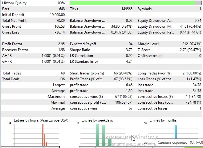
Let us examine the model’s performance on EURUSD M15, for the period starting July 1, 2025:

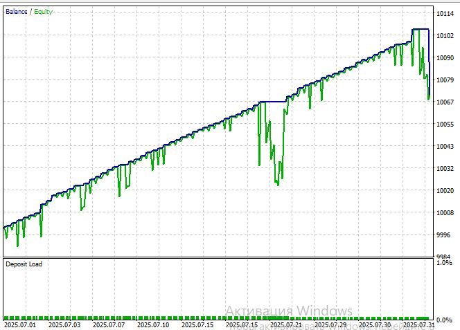
The Sharpe ratio turned out to be quite good:

Conclusion

The presented hybrid system demonstrates the practical feasibility of integrating modern deep learning architectures with classical econometric methods within the limitations of the MQL5 trading platform. A two-stage decomposition of the forecasting problem into linear and nonlinear components allows one to exploit the strengths of both approaches while minimizing their weaknesses.

Key achievements of the work include the successful adaptation of the U-Net architecture to financial time series analysis, the integration of attention mechanisms to model long-term dependencies, and the implementation of an automatic switching system between signal sources. The system demonstrates stable operation in various market conditions thanks to adaptive component weighting and periodic re-optimization of parameters.

The practical value of the solution lies in its readiness for use in real trading. The system includes a complete trading logic with position management, risk management, and detailed transaction logging. Separating symbols for analysis and trading expands the possibilities of using intermarket correlations.

However, the limitations of the current implementation should be honestly acknowledged. Simplified backpropagation, lack of modern regularization techniques, and fixed network architecture limit the potential of the neural network component. Using static arrays instead of dynamic data structures imposes severe limitations on the scalability of the system.

Nevertheless, the proposed approach opens up a promising direction for the development of trading systems. The concept of training a neural network on the residuals of a linear model can be applied to a wider class of forecasting problems, not limited to financial markets. The system's modular architecture allows for easy experimentation with different types of neural networks and position management strategies.

Of particular value is the demonstration that advanced machine learning techniques can be implemented even in limited development environments such as MQL5. This opens up opportunities for a wide range of traders and developers who do not have access to modern deep learning frameworks.

References

• Attention Is All You Need (Vaswani et al., 2017)
• U-Net: Convolutional Networks for Biomedical Image Segmentation (Ronneberger et al., 2015)