Neural Networks in Trading: Time Series Forecasting Using Adaptive Modal Decomposition (Final Part)

Introduction

In the previous article, we introduced the ACEFormer framework, a time-series forecasting model specifically adapted to the characteristics of financial markets. We examined the fundamental principles of probabilistic attention, the algorithms used to implement it at the OpenCL kernel level, and techniques for improving computational efficiency while preserving forecasting accuracy. However, one equally important aspect remained outside the scope of that discussion: how these mechanisms are integrated into the main program and how reliable communication is established between the computational module and the trading algorithm.

In this article, we continue implementing the approaches proposed by the authors of the ACEFormer framework. Our primary focus will be on building the corresponding algorithms on the program side. Before moving on to the technical implementation, however, let us briefly revisit the core concepts and strengths of ACEFormer. At the heart of the framework lies the ACEEMD (Alias Complete Ensemble Empirical Mode Decomposition with Adaptive Noise) algorithm, which is designed to remove noise from financial time series. ACEEMD effectively addresses the boundary effect while preserving the key turning points on the chart, without losing critical information during smoothing. Particular attention is given to the first intrinsic mode function (IMF), whose explicit removal helps eliminate high-frequency noise without excessively suppressing the useful signal.

The output of this stage is an adaptive modal representation of the time series, which serves as the input to the distillation module built on a Transformer architecture with probabilistic attention. This approach not only filters out market noise but also enables the model to focus on the truly informative regions of historical data, improving forecasting accuracy under conditions of high market volatility and stochasticity.

The processed representations are then passed through a conventional Self-Attention block, allowing the model to capture the global context of the original sequence and improve consistency across different time horizons. By combining localized probabilistic attention with global self-attention, the model is able to focus simultaneously on sharp market reversals and persistent trends.

The final stage of the architecture is a final prediction head, which transforms the high-level feature representation into a specific numerical forecast.

ACEFormer combines the strengths of two approaches: the robustness of empirical mode decomposition and the flexibility of deep attention mechanisms. At the same time, the model remains sufficiently compact for real-time deployment in user terminals and does not require excessive computational resources. Thanks to its modular architecture and support for parallel processing, ACEFormer can be readily adapted to a wide range of trading strategies, from short-term momentum models to medium-term position trading systems.

The authors' visualization of the ACEFormer framework is presented below.

Constructing the Probabilistic Attention Module

Having completed the implementation of the probabilistic attention mechanisms on the OpenCL program side, we now proceed to the next stage: developing the corresponding high-level module on the main program side. To accomplish this, we create a specialized CNeuronMHProbAttention object that encapsulates the complete probabilistic attention algorithm.

The new class inherits from CResidualConv, which already implements an architecture consisting of two consecutive convolutional layers connected through residual links. This allows us to focus exclusively on the implementation of the probabilistic attention logic without modifying the feed-forward mechanisms provided by the parent class. As a result, the design achieves a high degree of modularity while facilitating seamless integration with the other components of the model.

The structure of the new class is shown below.

class CNeuronMHProbAttention :  public CResidualConv
  {
protected:
   uint                       iWindow;
   uint                       iWindowKey;
   uint                       iHeads;
   uint                       iUnits;
   uint                       iTopKQuerys;
   uint                       iRandomKeys;
   int                        ibScore;
   //---
   CNeuronConvOCL             cQKV;
   CNeuronBaseOCL             cQ;
   CNeuronBaseOCL             cKV;
   CNeuronBaseOCL             cRandomK;
   CNeuronBaseOCL             cMHAttentionOut;
   CNeuronConvOCL             cPooling;
   CNeuronTransposeOCL        cTranspose[2];
   CNeuronConvOCL             cScaling;
   //---
   virtual bool               RandomKeys(CBufferFloat* indexes, int random, int units, int heads);
   virtual bool               QueryImportance(void);
   virtual bool               TopKIndexes(void);
   //---
   virtual bool               AttentionOut(void);
   virtual bool               AttentionInsideGradients(void);
   //---
   virtual bool               feedForward(CNeuronBaseOCL *NeuronOCL) override;
   virtual bool               updateInputWeights(CNeuronBaseOCL *NeuronOCL) override;
   virtual bool               calcInputGradients(CNeuronBaseOCL *prevLayer) override;

public:
                              CNeuronMHProbAttention(void) {};
                             ~CNeuronMHProbAttention(void) {};
   //---
   virtual bool               Init(uint numOutputs, uint myIndex, COpenCLMy *open_cl, 
                                   uint window, uint window_key, uint heads, uint units_count,
                                   ENUM_OPTIMIZATION optimization_type, uint batch);
   //---
   virtual int                Type(void)   const   {  return defNeuronMHProbAttention;   }
   //---
   virtual bool               Save(int const file_handle) override;
   virtual bool               Load(int const file_handle) override;
   //---
   virtual bool               WeightsUpdate(CNeuronBaseOCL *source, float tau) override;
   virtual void               SetOpenCL(COpenCLMy *obj) override;
  };

The structure of CNeuronMHProbAttention reflects the step-by-step implementation of the probabilistic attention mechanism, beginning with random key generation and query importance estimation, and ending with gradient backpropagation. Each functional component is implemented as a separate module, providing a clear separation of responsibilities and enabling fine-grained customization.

From an architectural perspective, one of the defining characteristics of CNeuronMHProbAttention is that all of its internal objects are declared statically. This design not only simplifies memory management but also eliminates the need for dynamic resource allocation when an instance of the class is created. Consequently, both the constructor and destructor remain empty, improving the reliability and predictability of object creation and destruction.

All required initialization of internal objects and variables is centralized in the Init method, which effectively serves as the class constructor. It is responsible for assembling all components, configuring their parameters, and allocating the required resources.

bool CNeuronMHProbAttention::Init(uint numOutputs, uint myIndex, COpenCLMy *open_cl,
                                  uint window, uint window_key, uint heads, uint units_count,
                                  ENUM_OPTIMIZATION optimization_type, uint batch
                                 )
  {
   if(!CResidualConv::Init(numOutputs, myIndex, open_cl, window, window, units_count, optimization_type, batch))
      return false;

Since the new class is derived from CResidualConv, which implements a residual convolutional architecture, the initialization procedure begins by calling the relevant method of the parent class. This immediately provides the underlying infrastructure, including the convolutional layers, residual connections, and buffer initialization. Consequently, we don't waste resources on reimplementation and can focus on the unique attention logic.

The next step is to initialize the key parameters that define the behavior of the attention mechanism.

iWindow = window;
iWindowKey = MathMax(5, window_key);
iHeads = MathMax(1, heads);
iUnits = units_count;
iTopKQuerys = int(MathMin(5 * MathMax(MathLog(iUnits),1), iUnits));
iRandomKeys = int(MathMin(5 * MathMax(MathLog(iUnits),1), iUnits));

In addition to the familiar parameters, two new variables specific to probabilistic attention are introduced:

• iTopKQuerys — the number of the most informative queries selected for further processing;
• iRandomKeys — the number of randomly sampled keys used during the query selection process.

To ensure scalability, the values of both parameters are computed as logarithmic functions of the total length of the input sequence.

Once the object parameters have been stored, the framework proceeds with the sequential construction of all internal components responsible for implementing the attention mechanism. Each object is initialized individually in a strictly defined order. The first component to be initialized is cQKV, a convolutional layer that simultaneously generates the three entities: Q (Query), K (Key), and V (Value). This layer produces dense feature representations for every attention head while encoding them using the TANH activation function.

int index = 0;
if(!cQKV.Init(0, index, OpenCL, iWindow, iWindow, 3 * iWindowKey * iHeads, iUnits, optimization, iBatch))
   return false;
cQKV.SetActivationFunction(TANH);

It is worth recalling that the previously developed kernels implementing probabilistic attention use a dedicated buffer for the Query tensor. Therefore, the next step is to create two additional objects that separate these entities.

index++;
if(!cQ.Init(0, index, OpenCL, cQKV.Neurons() / 3, optimization, iBatch))
   return false;
index++;
if(!cKV.Init(0, index, OpenCL, 2 * cQ.Neurons(), optimization, iBatch))
   return false;

The following object stores the randomly selected Key indices.

index++;
if(!cRandomK.Init(0, index, OpenCL, iHeads * MathMax(iRandomKeys, iTopKQuerys), optimization, iBatch))
   return false;

Notice that the size of this layer is determined by the larger of two values: the number of sampled Keys and the number of most important Queries. The idea is to guarantee sufficient memory capacity for all indices that may be required during computation. Since we cannot determine in advance which quantity will be larger — iRandomKeys for random Keys or iTopKQuerys for Queries — we allocate memory based on the maximum of the two. The resulting value is then multiplied by the number of attention heads (iHeads), as each head operates independently and therefore requires its own set of indices.

As a result, a single object cRandomK is used to store both the randomly sampled Key indices and the most informative Queries. This streamlines the module's internal structure, reduces the total number of objects, and simplifies memory management.

The next component stores the outputs of multi-head attention outputs for the most informative Queries.

index++;
if(!cMHAttentionOut.Init(0, index, OpenCL, iTopKQuerys * iHeads * iWindowKey, optimization, iBatch))
   return false;

This is followed by the adaptive aggregation layer, which combines the outputs of all attention heads into a unified representation.

index++;
if(!cPooling.Init(0, index, OpenCL, iHeads * iWindowKey, iHeads * iWindowKey, iWindow, iTopKQuerys,
                                                                              optimization, iBatch))
   return false;
cPooling.SetActivationFunction(TANH);

At this stage, the algorithm has already produced the output of the probabilistic attention mechanism. However, one important architectural consideration should be emphasized: these outputs correspond only to the selected Top-K Queries. Consequently, the resulting tensor has a substantially smaller temporal dimension than the original input sequence.

This creates an architectural mismatch. The probabilistic attention block produces a compressed representation, whereas the conventional Self-Attention architecture preserves the original sequence length. Maintaining this dimensional consistency is essential for correctly applying residual connections, which ensure stable training and effective gradient propagation.

To resolve this discrepancy, we adopt the following strategy:

• First, the attention output matrix is transposed so that its layout becomes suitable for convolution along the feature dimension.

index++;
if(!cTranspose[0].Init(0, index, OpenCL, iTopKQuerys, iWindow, optimization, iBatch))
   return false;

• Next, the convolutional layer cScaling is applied to restore the output to the original sequence length. As a result, the tensor regains the same dimensionality as the original input. Notably, this upscaling is performed independently for each feature, allowing every time step to be reconstructed while taking the global attention structure into account.

index++;
if(!cScaling.Init(0, index, OpenCL, iTopKQuerys, iTopKQuerys, iUnits, iWindow, optimization, iBatch))
   return false;
cScaling.SetActivationFunction(None);

• Finally, the data are returned to their original layout by applying a second transpose operation.

if(!cTranspose[1].Init(0, index, OpenCL, iWindow, iUnits, optimization, iBatch))
   return false;

This sequence of operations provides maximum compatibility between the stochastic probabilistic attention mechanism and the architectural requirements of conventional Self-Attention. The model preserves its structural integrity while maintaining the computational efficiency and flexibility required for stable training.

Special attention is paid to the ibScore buffer, which stores the intermediate attention scores required during backpropagation. This buffer is allocated exclusively within the OpenCL context.

   ibScore = OpenCL.AddBuffer(sizeof(float) * iTopKQuerys * iUnits * iHeads, CL_MEM_READ_WRITE);
   if(ibScore < 0)
      return false;
//---
   return true;
  }

After all internal objects have been initialized, the method completes by returning a logical success status.

The next major stage is the implementation of the feed-forward algorithm. Before processing the main data flow, however, a small amount of preparatory work is required.

As with most of the modules developed throughout this series, several methods simply enqueue OpenCL kernel executions. Since their underlying algorithms have already been discussed in previous articles, there is little value in repeating them here. Instead, we will focus on the Key sampling algorithm implemented in the RandomKeys method.

The objective of the probabilistic attention mechanism is to reduce the number of Keys that must be examined when identifying the most informative Queries. This lowers the computational cost while simultaneously introducing a stochastic component that helps mitigate overfitting and improves the model's generalization capability.

The RandomKeys method receives a pointer to the indexes buffer, which is to be populated with the sampled Key indices. The parameters random, units, and heads specify the number of random samples, the total number of available Keys, and the number of attention heads, respectively.

bool CNeuronMHProbAttention::RandomKeys(CBufferFloat *indexes, int random, int units, int heads)
  {
   if(!indexes || random > units ||
      indexes.Total() < (random * heads)
     )
      return false;

The method begins by validating the input parameters. If the buffer pointer is null, the requested number of random samples exceeds the number of available Keys, or the buffer is too small, the method immediately returns false.

Once the validation stage has been successfully completed, a random × heads matrix is created, where each column corresponds to an individual attention head and each row stores one sampled Key position.

matrix<float> ind = matrix<float>::Zeros(random, heads);

There are two possible scenarios further. If no sampling is required (random == units), the matrix is simply filled with consecutive indices, meaning that all available Keys are used.

if(random == units)
  {
   for(int r = 0; r < random; r++)
     {
      for(int c = 0; c < heads; c++)
         ind[r, c] = (float)r;
     }
  }

When the number of selected Keys (random) is smaller than the total number of available values (units), a naive random sampling strategy may produce an unrepresentative sample of available keys/data range. Simply drawing random indices from the entire range can result in duplicate values, local clusters, or, conversely, gaps where certain regions are not represented at all. As a result, the model may fail to observe important parts of the input sequence, negatively affecting the training process.

To avoid this issue, our implementation employs uniform stratified sampling. The entire index range is first divided into equally sized intervals.

else
  {
   double step = double(units) / random;

The result may be fractional, which is perfectly acceptable, since the sample size is rarely an exact divisor of the sequence length.

For each stratum (range segment), one value is selected at random from within its boundaries.

 for(int r = 0; r < random; r++)
   {
    for(int c = 0; c < heads; c++)
       ind[r, c] = float(int((r + MathRand() / 32767.0) * step));
   }
}

As a result, every attention head receives its own independently generated set of indices, while all of these sets collectively cover the entire sequence without a bias or excessive concentration in particular regions.

Once the sampling procedure has been completed, the sample is written to the indexes buffer, from which it is subsequently used in the OpenCL kernels.

   if(!indexes.AssignArray(ind) ||
      !indexes.BufferWrite())
      return false;
//---
   return true;
  }

This approach offers several important advantages. First, it guarantees uniform coverage of the entire feature space. Second, it prevents indices from falling outside the valid range while minimizing the likelihood of duplicate samples. Consequently, the sampled subset becomes substantially more representative, providing the model with a more complete and balanced view of the original data. This is particularly important when working with financial time series, where periods of low volatility can be just as informative as episodes of rapid market movement.

With the preparatory stage complete, we can proceed to the core of the implementation — the feedForward method, which performs the full probabilistic attention algorithm.

bool CNeuronMHProbAttention::feedForward(CNeuronBaseOCL *NeuronOCL)
  {
   if(!cQKV.FeedForward(NeuronOCL))
      return false;

The first operation calls the FeedForward method of the cQKV convolutional layer. As its name suggests, this layer generates a concatenated tensor containing Query, Key, and Value representations. The output is a single tensor in which the three components are stored sequentially.

For the subsequent stages of the algorithm, however, these representations must be separated into two tensors: one containing the Queries (Q), and another containing the Keys and Values (K and V). This is done by using the DeConcat method, which extracts the corresponding portions of the combined QKV tensor and transfers them to cQ and cKV.

if(!DeConcat(cQ.getOutput(), cKV.getOutput(), cQKV.getOutput(), iWindowKey * iHeads,
                                                    2 * iWindowKey * iHeads, iUnits))
   return false;

The previously described Key sampling algorithm is then executed by calling the RandomKeys method.

if(!RandomKeys(cRandomK.getOutput(), iRandomKeys, iUnits, iHeads))
   return false;

The next stage invokes the QueryImportance and TopKIndexes methods. These methods enqueue kernels responsible for ranking Query importance and selecting the most informative ones.

if(!QueryImportance() || !TopKIndexes())
   return false;

The core of the algorithm follows in the AttentionOut method. It enqueues the attention kernel responsible for computing attention only for the selected Queries.

if(!AttentionOut())
   return false;

The resulting outputs from all attention heads are then aggregated by the cPooling convolutional layer. This layer also applies the TANH activation function, increasing the expressive power of the output signal.

if(!cPooling.FeedForward(cMHAttentionOut.AsObject()))
   return false;

The aggregated outputs are subsequently upscaled to restore the tensor to the dimensionality of the original input sequence, allowing residual connections to be applied correctly.

if(!cTranspose[0].FeedForward(cPooling.AsObject()))
   return false;
if(!cScaling.FeedForward(cTranspose[0].AsObject()))
   return false;
if(!cTranspose[1].FeedForward(cScaling.AsObject()))
   return false;

The final operation within the attention block calls the SumAndNormalize method, which combines the upscaled representation with the original input by adding the residual connection and performing normalization. This ensures stable gradient propagation and accelerates convergence during training.

if(!SumAndNormilize(cTranspose[1].getOutput(), NeuronOCL.getOutput(), cTranspose[1].getOutput(),
                    iWindow, true, 0, 0, 0, 1))
   return false;

Finally, the resulting tensor is passed to the corresponding method of the parent class, which completes the forward propagation stage and returns the output tensor, ready to be processed by the next module of the neural network.

 return CResidualConv::feedForward(cTranspose[1].AsObject());
}

As a result, the entire probabilistic attention mechanism is encapsulated in the CNeuronMHProbAttention object. This design provides a highly modular, reusable, and easily scalable implementation.

Once the feed-forward pass has been completed, the training process enters its most critical phase: backpropagation of the optimization error gradient to update the model parameters. During this stage, the contribution of every component to the overall loss is computed, after which the network weights are adjusted accordingly. In the case of the probabilistic attention mechanism implemented by the CNeuronMHProbAttention class, backpropagation becomes considerably more sophisticated because gradients are propagated only through the subset of selected Queries. This requires careful organization of the process and strict adherence to the computational logic.

bool CNeuronMHProbAttention::calcInputGradients(CNeuronBaseOCL *prevLayer)
  {
   if(!prevLayer)
      return false;

The calcInputGradients method begins with a basic validation of the pointer to the preceding layer, which is received as one of the method's parameters. Without a valid reference to the previous layer, the error gradient cannot be propagated further through the network.

The next step is an important preparatory operation: the Query gradient buffer is explicitly cleared.

if(!cQ.getGradient().Fill(0))
   return false;

This operation is mandatory because the attention algorithm processes only a subset of Queries — the most relevant ones selected during the feed-forward pass. The remaining elements of the gradient matrix may still contain stale or undefined values that are no longer valid and could corrupt subsequent parameter updates. Therefore, the entire matrix is cleared before the correct gradient values begin to accumulate.

Next, we call the corresponding method of the parent class. This operation propagates the error through the FeedForward block. Thus, this portion of the backpropagation pass is delegated to the already proven logic.

if(!CResidualConv::calcInputGradients(cTranspose[1].AsObject()))
   return false;

Further steps propagate the error gradients sequentially through every internal block of the probabilistic attention mechanism, exactly mirroring the structure of the feed-forward pass, but in reverse order. The gradients first pass through the scaling block.

if(!cScaling.calcHiddenGradients(cTranspose[1].AsObject()))
   return false;
if(!cTranspose[0].calcHiddenGradients(cScaling.AsObject()))
   return false;

They are then propagated through the multi-head attention aggregation layer.

if(!cPooling.calcHiddenGradients(cTranspose[0].AsObject()))
   return false;
if(!cMHAttentionOut.calcHiddenGradients(cPooling.AsObject()))
   return false;

These stages are essential for accurately reconstructing the gradients because the feed-forward pass involved multiple transformations of data shape and structure. Now these operations must be reversed in the correct order.

Particular attention is paid to the AttentionInsideGradients method, which performs gradient propagation within the probabilistic attention mechanism itself. This is where the error is carefully propagated through the subset of selected Queries. It is the most sensitive component of the entire backpropagation pass: it preserves weight updates accurate and mathematically consistent, even though only a fraction of the original information participates in the process.

if(!AttentionInsideGradients())
   return false;

The next stage merges the gradients by combining the Query, Key, and Value gradients into a single QKV tensor, restoring the original representation produced during the feed-forward pass. If an activation function was applied in the cQKV block, the gradients are corrected by calculating the derivative of this function. This accounts for its influence on the propagated signals and preserves the mathematical correctness of the entire process.

if(!Concat(cQ.getGradient(), cKV.getGradient(), cQKV.getGradient(), iWindowKey * iHeads,
                                                        2 * iWindowKey * iHeads, iUnits))
   return false;
if(cQKV.Activation() != None)
   if(!DeActivation(cQKV.getOutput(), cQKV.getGradient(), cQKV.getGradient(), cQKV.Activation()))
      return false;

The gradients obtained at this stage are then passed to the preceding layer.

if(!prevLayer.calcHiddenGradients(cQKV.AsObject()))
   return false;

The only remaining component is the error gradient flowing through the residual connection. First, this gradient is corrected using the derivative of the activation function applied to the original input layer. The gradients from the two branches are then summed.

   if(prevLayer.Activation() != None)
      if(!DeActivation(prevLayer.getOutput(), cTranspose[1].getGradient(), cTranspose[1].getGradient(),
                                                                               prevLayer.Activation()))
         return false;
   if(!SumAndNormilize(cTranspose[1].getGradient(), prevLayer.getGradient(), prevLayer.getGradient(),
                       iWindow, false, 0, 0, 0, 1))
      return false;
//---
   return true;
  }

As a result, the calcInputGradients method implements the complete backpropagation algorithm for the probabilistic attention module. It preserves the accuracy and consistency of every gradient transformation, enabling the probabilistic attention mechanism to be integrated into complex neural network architectures without the risk of information loss or distortion of the training signal.

The final stage of the training process involves updating the model parameters and is implemented by the updateInputWeights method. Since all trainable parameters are located in internal objects, the implementation simply consists of sequentially calling the corresponding update methods of those components. The implementation is straightforward, so this method is not discussed in detail in this article. The complete source code of the probabilistic attention module, including the updateInputWeights method, is provided in the attachments.

Model Architecture

In conclusion of the review of the basic implementation components, it is worth examining the overall architecture of the training system. As in several of our previous works, we adopt a hierarchical learning framework based on the Actor–Director–Critic paradigm. This approach provides a clear separation between environment processing, decision-making, and action evaluation, which is particularly important in the context of complex and highly dynamic financial markets.

Within this framework, four models are trained. The first — the Environment State Encoder — plays the central role. It is responsible for performing a deep analysis of the market situation and constructing its compact yet highly informative latent representation. This model uses the techniques proposed by the ACEFormer framework to predict future environment states over a specified planning horizon. As a result, it produces a stable and dynamically meaningful market representation that subsequently serves as the foundation for the Agent's actions.

The second model — the Actor — operates on two sources of information simultaneously. The first consists of the current account state and open positions, while the second is the latent environment representation generated by the Encoder. The Actor is trained to select actions that best match the current market conditions, and its decisions are subsequently evaluated by the remaining two models.

The Director and Critic models evaluate the actions selected by the Actor. The Director introduces a strict binary filtering mechanism that helps eliminate strategically unfavorable decisions, whereas the Critic provides a softer, quantitative assessment by estimating the expected utility of the selected actions. Together, these two components enable the agent to develop a robust and adaptive trading strategy.

In this article, we focus on the architecture of the Environment State Encoder, since it is the component that incorporates the key elements of the ACEFormer framework. The architectures of the remaining models generally follow the principles described in our previous publications.

As usual, the input layer consists of a fully connected layer of sufficient size.

//--- Encoder
   encoder.Clear();
//--- Input layer
   if(!(descr = new CLayerDescription()))
      return false;
   descr.type = defNeuronBaseOCL;
   int prev_count = descr.count = (HistoryBars * BarDescr);
   descr.activation = None;
   descr.optimization = ADAM;
   if(!encoder.Add(descr))
     {
      delete descr;
      return false;
     }

It is worth noting that, unlike the original ACEFormer implementation, we do not append zero values for the forecasted elements.

The first stage of data processing is performed by a dedicated feature preprocessing module. This module combines normalization with stochastic noise injection and a convolutional transformation of the feature dimensionality.

The process begins by normalizing the input data. This removes differences in scale between individual features and stabilizes the training process. To further improve the model's generalization capability and robustness to local data fluctuations, a controlled amount of random noise is introduced during normalization. This acts as a regularization mechanism by simulating the variability of real market conditions, allowing the model to better adapt to unstable or previously unseen scenarios.

The normalized and noise-augmented data are then passed through a convolutional layer that transforms the feature dimensionality into the format required by the subsequent network components. This operation simultaneously reduces redundant information and extracts the most relevant spatial relationships between features within the specified temporal window.

//--- layer 1
   if(!(descr = new CLayerDescription()))
      return false;
   descr.type = defNeuronBatchNormWithNoise;
   descr.count = prev_count;
   descr.batch = 1e4;
   descr.activation = None;
   descr.optimization = ADAM;
   if(!encoder.Add(descr))
     {
      delete descr;
      return false;
     }
//--- layer 2
   if(!(descr = new CLayerDescription()))
      return false;
   descr.type = defNeuronConvOCL;
   prev_count = descr.count = HistoryBars;
   descr.window = BarDescr;
   descr.step = BarDescr;
   int prev_out = descr.window_out = NSkills;
   descr.batch = 1e4;
   descr.optimization = ADAM;
   descr.activation = None;
   if(!encoder.Add(descr))
     {
      delete descr;
      return false;
     }

Following preprocessing, the data are transposed to switch from temporal analysis to independent feature analysis. This enables the attention mechanism to identify meaningful dependencies within each feature, improving the representations and the training process.

//--- layer 3
   if(!(descr = new CLayerDescription()))
      return false;
   descr.type = defNeuronTransposeOCL;
   descr.count = prev_count;
   prev_count = descr.window = prev_out;
   prev_out = descr.count;
   descr.batch = 1e4;
   descr.optimization = ADAM;
   descr.activation = None;
   if(!encoder.Add(descr))
     {
      delete descr;
      return false;
     }

Next we move on to the distillation block. In the Encoder architecture, it implements the central idea of the ACEFormer framework: extracting the most informative features and aggregating the meaningful information. At its core is the probabilistic attention module, which processes the input first by focusing on the most significant features. This enables the model to concentrate on the most informative components of the original signal.

//--- layer 4
   if(!(descr = new CLayerDescription()))
      return false;
   descr.type = defNeuronMHProbAttention;
   descr.count = prev_count;
   descr.window = prev_out;
   descr.step = 4;
   descr.window_out = 32;
   descr.batch = 1e4;
   descr.optimization = ADAM;
   descr.activation = None;
   if(!encoder.Add(descr))
     {
      delete descr;
      return false;
     }

Immediately after the attention module comes a convolutional layer that reduces the temporal dimension of the features. Its purpose is to compress the information while preserving its essential characteristics.

//--- layer 5
   if(!(descr = new CLayerDescription()))
      return false;
   descr.type = defNeuronConvOCL;
   prev_out = descr.count = (prev_out + 1) / 2;
   descr.window = 2;
   descr.step = 2;
   int filt=descr.window_out = 5;
   descr.layers = prev_count;
   descr.batch = 1e4;
   descr.optimization = ADAM;
   descr.activation = None;
   if(!encoder.Add(descr))
     {
      delete descr;
      return false;
     }

This is followed by an aggregation module that operates similarly to a max-pooling layer, selecting the strongest activations within each window and preserving the dominant features.

//--- layer 6
   if(!(descr = new CLayerDescription()))
      return false;
   descr.type = defNeuronProofOCL;
   descr.count = prev_count*prev_out;
   descr.window = filt;
   descr.step = filt;
   descr.layers = prev_count;
   descr.batch = 1e4;
   descr.optimization = ADAM;
   descr.activation = None;
   if(!encoder.Add(descr))
     {
      delete descr;
      return false;
     }

Finally, a normalization layer stabilizes the feature distribution and accelerates the training process.

//--- layer 7
   if(!(descr = new CLayerDescription()))
      return false;
   descr.type = defNeuronBatchNormOCL;
   descr.count = prev_count * prev_out;
   descr.batch = 1e4;
   descr.activation = None;
   descr.optimization = ADAM;
   if(!encoder.Add(descr))
     {
      delete descr;
      return false;
     }

Our implementation employs three consecutive distillation blocks, each independently reducing the dimensionality of the individual feature time series.

//--- layer 8
   if(!(descr = new CLayerDescription()))
      return false;
   descr.type = defNeuronMHProbAttention;
   descr.count = prev_count;
   descr.window = prev_out;
   descr.step = 4;
   descr.window_out = 32;
   descr.batch = 1e4;
   descr.optimization = ADAM;
   descr.activation = None;
   if(!encoder.Add(descr))
     {
      delete descr;
      return false;
     }
//--- layer 9
   if(!(descr = new CLayerDescription()))
      return false;
   descr.type = defNeuronConvOCL;
   prev_out = descr.count = (prev_out + 1) / 2;
   descr.window = 2;
   descr.step = 2 ;
   filt=descr.window_out = 3;
   descr.layers = prev_count;
   descr.batch = 1e4;
   descr.optimization = ADAM;
   descr.activation = None;
   if(!encoder.Add(descr))
     {
      delete descr;
      return false;
     }
//--- layer 10
   if(!(descr = new CLayerDescription()))
      return false;
   descr.type = defNeuronProofOCL;
   descr.count = prev_count*prev_out;
   descr.window = filt;
   descr.step = filt;
   descr.layers = prev_count;
   descr.batch = 1e4;
   descr.optimization = ADAM;
   descr.activation = None;
   if(!encoder.Add(descr))
     {
      delete descr;
      return false;
     }
//--- layer 11
   if(!(descr = new CLayerDescription()))
      return false;
   descr.type = defNeuronBatchNormOCL;
   descr.count = prev_count * prev_out;
   descr.batch = 1e4;
   descr.activation = None;
   descr.optimization = ADAM;
   if(!encoder.Add(descr))
     {
      delete descr;
      return false;
     }

//--- layer 12
   if(!(descr = new CLayerDescription()))
      return false;
   descr.type = defNeuronMHProbAttention;
   descr.count = prev_count;
   descr.window = prev_out;
   descr.step = 4;
   descr.window_out = 32;
   descr.batch = 1e4;
   descr.optimization = ADAM;
   descr.activation = None;
   if(!encoder.Add(descr))
     {
      delete descr;
      return false;
     }
//--- layer 13
   if(!(descr = new CLayerDescription()))
      return false;
   descr.type = defNeuronConvOCL;
   prev_out = descr.count = (prev_out + 1) / 2;
   descr.window = 2;
   descr.step = 2 ;
   filt=descr.window_out = 3;
   descr.layers = prev_count;
   descr.batch = 1e4;
   descr.optimization = ADAM;
   descr.activation = None;
   if(!encoder.Add(descr))
     {
      delete descr;
      return false;
     }
//--- layer 14
   if(!(descr = new CLayerDescription()))
      return false;
   descr.type = defNeuronProofOCL;
   descr.count = prev_count*prev_out;
   descr.window = filt;
   descr.step = filt;
   descr.layers = prev_count;
   descr.batch = 1e4;
   descr.optimization = ADAM;
   descr.activation = None;
   if(!encoder.Add(descr))
     {
      delete descr;
      return false;
     }
//--- layer 15
   if(!(descr = new CLayerDescription()))
      return false;
   descr.type = defNeuronBatchNormOCL;
   descr.count = prev_count * prev_out;
   descr.batch = 1e4;
   descr.activation = None;
   descr.optimization = ADAM;
   if(!encoder.Add(descr))
     {
      delete descr;
      return false;
     }

Thus, the distillation block not only reduces dimensionality, it extracts and concentrates the essence of the original data, producing a rich latent representation that is robust to noise.

The Encoder architecture then incorporates a two-layer Self-Attention block whose purpose is to capture dependencies between features within the compressed latent representation. This helps discover hidden relationships and synchronize information across different feature dimensions.

//--- layer 16
   if(!(descr = new CLayerDescription()))
      return false;
   descr.type = defNeuronDMHAttention;
   descr.count = prev_count;
   descr.window = prev_out;
   descr.step = 4;
   descr.layers = 2;
   descr.window_out = 32;
   descr.batch = 1e4;
   descr.optimization = ADAM;
   descr.activation = None;
   if(!encoder.Add(descr))
     {
      delete descr;
      return false;
     }

As a result, the model learns to perceive the data not merely as a collection of independent observations, but as a coherent system of interacting components.

To independently forecast each individual feature sequence, the Encoder uses two consecutive convolutional layers. This design efficiently transforms the generalized latent representation into numerical predictions for every target feature.

The first convolutional layer uses an expanded number of filters (4 times the number of forecasted parameters) and applies the SoftPlus activation function. This produces a smooth positive-values transformation that improves training stability while suppressing noise.

//--- layer 17
   if(!(descr = new CLayerDescription()))
      return false;
   descr.type = defNeuronConvOCL;
   descr.count = 1;
   descr.window = prev_out;
   descr.step = prev_out;
   prev_out = descr.window_out = 4 * NForecast;
   descr.layers = prev_count;
   descr.activation = SoftPlus;
   if(!encoder.Add(descr))
     {
      delete descr;
      return false;
     }

The second layer completes the decoding process by reducing the number of outputs to exactly the number of predicted parameters (NForecast) and applies the TANH activation function. This helps keep the predictions within a controlled value range, which is particularly important when working with normalized data.

//--- layer 18
   if(!(descr = new CLayerDescription()))
      return false;
   descr.type = defNeuronConvOCL;
   descr.count = 1;
   descr.window = prev_out;
   descr.step = prev_out;
   prev_out = descr.window_out = NForecast;
   descr.layers = prev_count;
   descr.activation = TANH;
   if(!encoder.Add(descr))
     {
      delete descr;
      return false;
     }

This architecture is simple yet effective. It provides sufficient flexibility for generating accurate forecasts while preserving the independence of individual feature predictions — a critical property when modeling financial time series, where each variable may carry unique information.

At the final stage of the Encoder, the predicted values are transformed back into the original data space, allowing the model outputs to be interpreted.

The first operation is a tensor transpose. It restores the temporal dimension to its original orientation and aligns the forecast values with their corresponding time steps.

//--- layer 19
   if(!(descr = new CLayerDescription()))
      return false;
   descr.type = defNeuronTransposeOCL;
   descr.count = prev_count;
   prev_count=descr.window = prev_out;
   prev_out=descr.count;
   descr.activation = None;
   if(!encoder.Add(descr))
     {
      delete descr;
      return false;
     }

Next, a convolutional layer projects the feature dimensionality back into the format of the original input data. In essence, this is a projection: the model compresses or expands the latent representation so that it becomes compatible with the space in which the original data was formed.

//--- layer 20
   if(!(descr = new CLayerDescription()))
      return false;
   descr.type = defNeuronConvOCL;
   descr.count = prev_count;
   descr.window = prev_out;
   descr.step = prev_out;
   prev_out = descr.window_out = BarDescr;
   descr.layers = 1;
   descr.activation = TANH;
   if(!encoder.Add(descr))
     {
      delete descr;
      return false;
     }

Finally, inverse normalization converts the predictions from the model's internal normalized representation back into real-world values that can be interpreted by users and employed directly in trading decisions.

//--- layer 21
   if(!(descr = new CLayerDescription()))
      return false;
   descr.type = defNeuronRevInDenormOCL;
   descr.count = prev_count * prev_out;
   descr.layers = 1;
   descr.activation = None;
   if(!encoder.Add(descr))
     {
      delete descr;
      return false;
     }

Together, these operations bridge the gap between the model's internal representation and the real market, transforming abstract latent predictions into actionable forecasts.

The complete architectures of all trainable models are provided in the attachments.

Testing

A significant amount of work has been devoted to adapting and implementing the ACEFormer framework in the MQL5 environment. The framework's core components have now been integrated into the architecture of the trainable models. The next step is to evaluate the resulting models on real historical data.

The training dataset was generated by running the MetaTrader 5 Strategy Tester with random agent policies on one-minute EURUSD price data for the entire year of 2024. This approach exposes the models to a broad range of market scenarios and improves the generality of the learned behavior.

Training was performed in two stages. The first stage is offline training without updating the dataset until the optimization errors had stabilized. To do this, we ran the Study.mq5 Expert Advisor on the chart. The second stage employed online training in the Strategy Tester using the StudyOnline.mq5 Expert Advisor, allowing the models to be fine-tuned under conditions that closely resemble real trading.

To objectively evaluate the results, the trained models were tested on out-of-sample historical data covering January through March 2025. This eliminates overfitting and emphasizes the practical value of the results obtained.

All other environment parameters and technical indicators remained unchanged throughout both training and testing, ensuring that the observed results reflect the quality of the learned strategy.

The testing results are presented below.

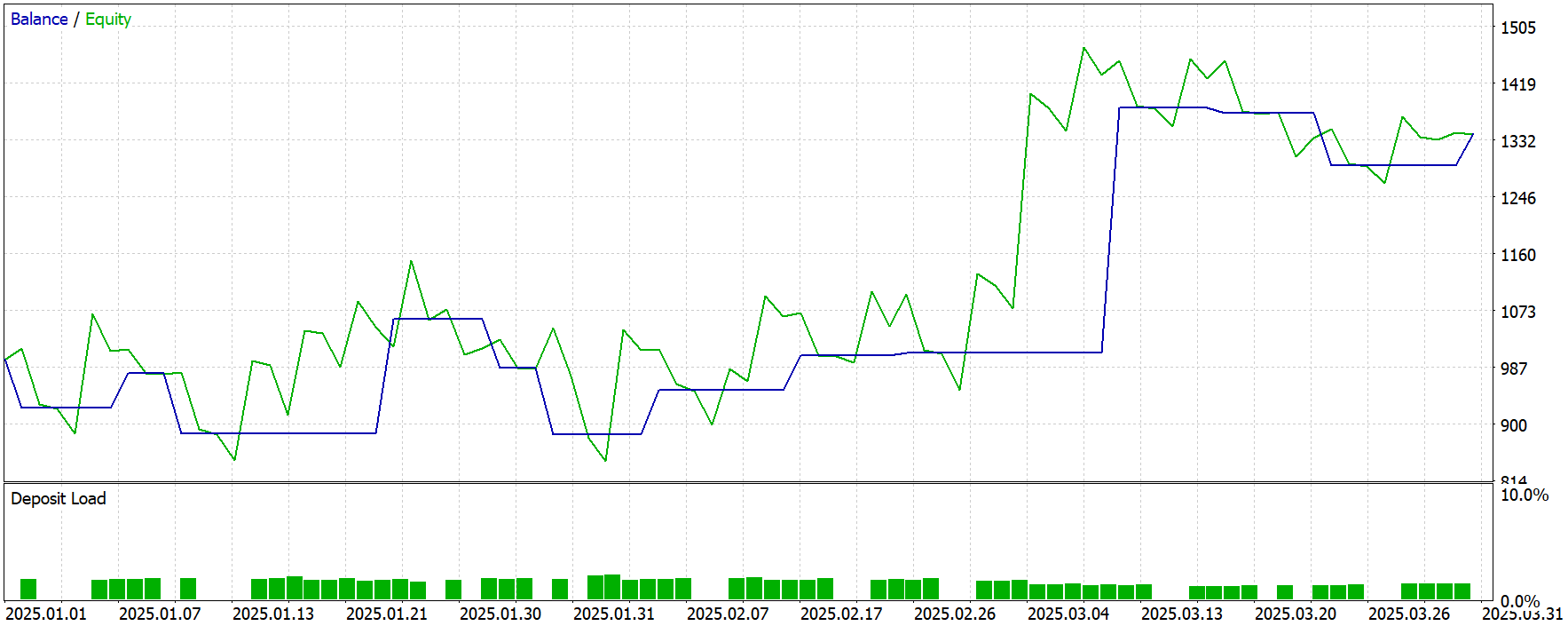
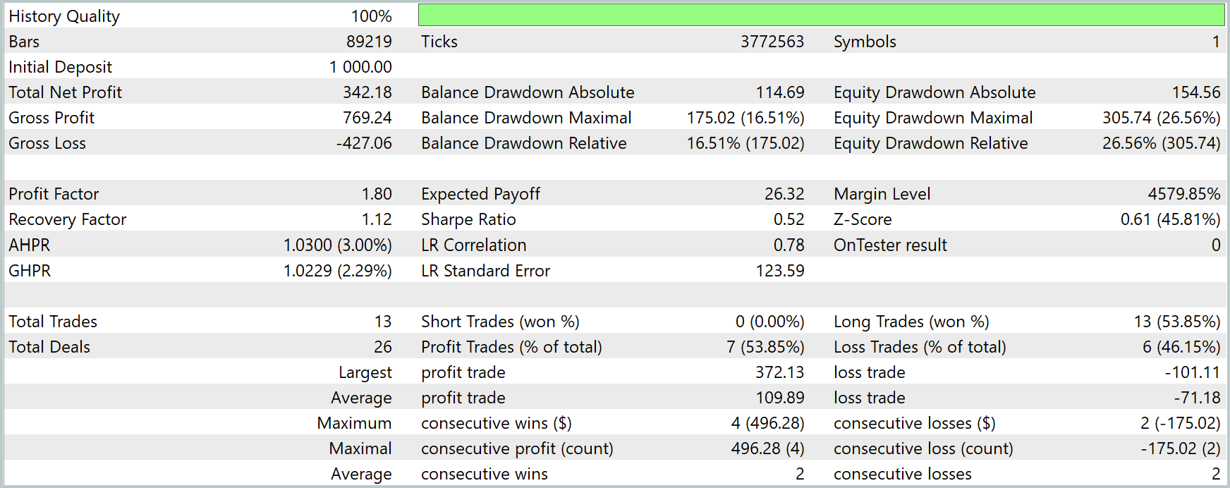
Overall, the model was profitable over the testing period, executing 13 trades. Slightly more than half of those trades were profitable. However, it should be noted that 13 trades over a three-month evaluation period represents relatively low trading activity.

One possible explanation is the nature of the probabilistic attention mechanism itself. By selecting only the most informative features and Queries, the model achieves better generalization but may become less sensitive to weaker trading signals.

Another contributing factor may be the limited representativeness of the training dataset. The model may simply not have encountered a sufficiently diverse range of market conditions during training to act confidently in similar situations throughout the evaluation period. Expanding both the size and diversity of the training data could improve the agent's behavioral flexibility.

Conclusion

In this article, we explored the ACEFormer framework, which provides an effective approach for extracting informative features from time series and constructing compact latent representations. Its architecture combines probabilistic attention, feature distillation, and deep sequence transformation, making it particularly well suited for analyzing noisy and highly volatile financial data.

From a practical perspective, we presented our own implementation of the key ACEFormer components using MQL5 and integrated them into a trainable Actor–Director–Critic architecture. Particular attention was devoted to the design of the Environment State Encoder, which implements the feature-processing techniques proposed by the framework.

The experimental results were encouraging: the model generated a positive return on the out-of-sample test period, confirming the overall viability of the proposed architecture. At the same time, the experiments revealed relatively low trading activity, which may stem from the characteristics of probabilistic attention and the limited diversity of the training dataset. These observations provide a clear direction for future research.

References

• An End-to-End Structure with Novel Position Mechanism and Improved EMD for Stock Forecasting
• Other articles from this series

Programs Used in the Article

#	Name	Type	Description
1	Research.mq5	Expert Advisor	Expert Advisor for collecting samples
2	ResearchRealORL.mq5	Expert Advisor	Expert Advisor for collecting samples using the Real-ORL method
3	Study.mq5	Expert Advisor	Expert Advisor for offline model training
4	StudyOnline.mq5	Expert Advisor	Expert Advisor for online model training
4	Test.mq5	Expert Advisor	Expert Advisor for model testing
5	Trajectory.mqh	Class library	System state and model architecture description structure
6	NeuroNet.mqh	Class library	A library of classes for creating a neural network
7	NeuroNet.cl	Code library	OpenCL program code