Neural networks made easy (Part 45): Training state exploration skills

Introduction

Hierarchical reinforcement learning algorithms can successfully solve quite complex problems. This is achieved by dividing the problem into smaller sub-tasks. One of the main problems in this context is the correct selection and training of skills that allow the agent to act effectively and, if possible, manage the environment as much as possible to achieve the goal.

Previously, we already got acquainted with DIAYN and DADS skill training algorithms. In the first case, we taught skills with maximum variety of behaviors willing to ensure maximum exploration of the environment. At the same time, we were willing to train skills that were not useful for our current task.

In the second algorithm (DADS), we approached learning skills from the perspective of their impact on the environment. Here we aimed to predict environmental dynamics and use skills that allow us to gain maximum benefit from changes.

In both cases, the skills from the prior distribution were used as input to the agent and explored during the training process. The practical use of this approach demonstrates insufficient coverage of the state space. Consequently, trained skills are not able to effectively interact with all possible environmental states.

In this article, I propose to get acquainted with the alternative method of teaching skills Explore, Discover and Learn (EDL). EDL approaches the problem from a different angle, which allows it to overcome the problem of limited state coverage and offer more flexible and adaptive agent behavior.

1. "Explore, Discover and Learn" algorithm

Exploration, Discovery, and Learning (EDL) method was presented in the scientific article "Explore, Discover and Learn: Unsupervised Discovery of State-Covering Skills" in August 2020. It proposes an approach that allows an agent to discover and learn to use different skills in an environment without any prior knowledge of states and skills. It also allows for the training of a variety of skills spanning different states, allowing for more efficient exploration and learning of an agent in an unknown environment.

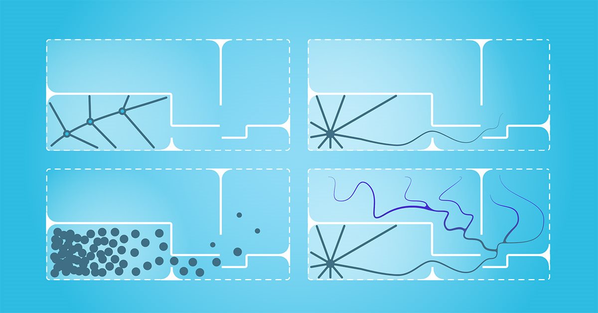
The EDL method has a fixed structure and consists of three main stages: exploration, discovery and skill training.

We start our exploration without any prior knowledge of the environment and the required skills. At this stage, we have to create a training set of initial states with maximum coverage of various states corresponding to all possible environmental behavior. In our work, we will use a uniform sampling of system states during the training period. However, other approaches are also possible, especially when training specific modes of agent behavior. It should be noted that EDL does not require access to the trajectories or actions made by the expert strategy. But it does not exclude their use either.

At the second stage, we search for skills hidden in specific environmental conditions. The fundamental idea of this method is that there is some connection between the state (or state space) of the environment and the specific skill that the agent should use. We have to determine such dependencies.

It should be noted that at this stage we do not have any knowledge about environmental conditions. There is only a sample of such states. Moreover, we lack knowledge about the necessary skills. At the same time, we previously noted that the EDL method involves the discovery of skills without a teacher. The algorithm uses variational auto encoder to search for the specified dependencies. There will be environmental states at the model input and output. In the latent state of the auto encoder, we expect to obtain the identification of a latent skill that follows from the current state of the environment. In this approach, the encoder of our auto encoder builds a function of how the skill depends on the current state of the environment. The model decoder performs the inverse function and builds a dependence of the state on the skill used. Using a variational auto encoder allows us to move from a clear "state-skill" correspondence to a certain probability distribution. This generally increases the stability of the model in a complex stochastic environment.

Thus, in the absence of additional knowledge about states and skills, the use of variational auto encoder in the EDL method provides us with the opportunity to explore and discover hidden skills associated with different environmental states. Building a function of the relationship between the state of the environment and the required skill will allow us to interpret new states of the environment into a set of the most relevant skills in the future.

Note that in the previously discussed methods, we trained the skills first. Then the scheduler looked for a strategy to use ready-made skills to achieve the goal. The EDL method takes the opposite approach. We first build dependencies between state and skills. After that, we teach the skills. This allows us to more accurately match skills to specific environmental conditions and determine which skills are most effective to use in certain situations.

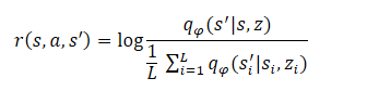
The final stage of the algorithm is training the skill model (Agent). Here, the agent learns a strategy that maximizes mutual information between states and hidden variables. The agent is trained using reinforcement learning methods. The formation of the reward is structured similarly to the DADS method, but the method authors slightly simplified the equation. As you might remember, the agent internal reward in DADS was formed according to the equation:

From the math course, we know that

Hence:

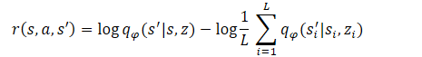
As you can see, the subtrahend is a constant for all skills used. Therefore, we can only use the minuend to optimize the policy. This approach allows us to reduce the amount of calculations without losing the quality of model training.

This final step can be thought of as training a strategy that imitates the decoder under a Markov decision process, that is, a strategy that will visit the states that the decoder will generate for each hidden z skill. It should be noted that the reward function is fixed, unlike previous methods, in which it continuously changes depending on the strategy behavior. This makes training more stable and increases the convergence of models.

2. Implementation using MQL5

After considering the theoretical aspects of the Exploration, Discovery and Learning (EDL) method, let's move on to the practical part of our article. Before implementing the method using MQL5, we need to have a look at the implementation features.

In the Test section of the previous article, we demonstrated the similarity of the results of using the one-hot vector and the full distribution to identify the skill used in the Agent’s source data. This allows us to use one approach or another depending on the data we have to reduce the math involved. This in general gives us the potential to reduce the number of operations performed. At the same time, we are able to increase the speed of model training and operation.

The second point we need to pay attention to is that we submit the same initial data to the input of the Scheduler and the Agent (historical data on price movement, parameter values and balance state). The skill ID is also added to this data at the Agent input.

On the other hand, when studying auto encoders, we mentioned that the latent state of an auto encoder is a compressed representation of its original data. In other words, by concatenating the vector of source data with the vector of latent data of the variational auto encoder, we pass the same data twice in its full and compressed representation.

If similar blocks of preliminary source data handling are used, this approach may be redundant. So, in this implementation, we will only send the latent state of the auto encoder to the Agent’s input, which already contains all the necessary information. This will allow us to significantly reduce the volume of operations performed, as well as the total time for training models.

Of course, this approach is only possible when using similar initial data at the input of the Scheduler and Agent. Other options are possible as well. For example, the auto encoder can build dependencies only between historical data and a skill without taking into account the state of the account. At the agent’s input, it is able to concatenate the vector of the latent state of the auto encoder and the vector of description of the counting state. It would not be a mistake to use all the data, as we did when implementing the previously discussed methods. You can experiment with different approaches in your implementation.

All such decisions are necessarily reflected in the model architecture we specify in the CreateDescriptions function. In the method parameters, we pass pointers to 2 dynamic arrays describing the scheduler and agent models. Please note that we do not create a Discriminator when implementing the EDL method, since its role is played by the auto encoder (Scheduler) decoder.

bool CreateDescriptions(CArrayObj *actor, CArrayObj *scheduler)
  {
//---
   CLayerDescription *descr;
//---
   if(!actor)
     {
      actor = new CArrayObj();
      if(!actor)
         return false;
     }
//---
   if(!scheduler)
     {
      scheduler = new CArrayObj();
      if(!scheduler)
         return false;
     }

The variational auto encoder for the Scheduler is created first. We feed this model with historical data and account status, which is reflected in the size of the source data layer. As always, the raw data is pre-processed in a batch normalization layer.

//--- Scheduler
   scheduler.Clear();
//--- Input layer
   if(!(descr = new CLayerDescription()))
      return false;
   descr.type = defNeuronBaseOCL;
   int prev_count = descr.count = (HistoryBars * BarDescr + AccountDescr);
   descr.window = 0;
   descr.activation = None;
   descr.optimization = ADAM;
   if(!scheduler.Add(descr))
     {
      delete descr;
      return false;
     }
//--- layer 1
   if(!(descr = new CLayerDescription()))
      return false;
   descr.type = defNeuronBatchNormOCL;
   descr.count = prev_count;
   descr.batch = 1000;
   descr.activation = None;
   descr.optimization = ADAM;
   if(!scheduler.Add(descr))
     {
      delete descr;
      return false;
     }

Next comes a convolutional block to reduce the dimensionality of the data and extract specific features.

//--- layer 2
   if(!(descr = new CLayerDescription()))
      return false;
   descr.type = defNeuronConvOCL;
   prev_count = descr.count = prev_count - 1;
   descr.window = 2;
   descr.step = 1;
   descr.window_out = 4;
   descr.activation = LReLU;
   descr.optimization = ADAM;
   if(!scheduler.Add(descr))
     {
      delete descr;
      return false;
     }
//--- layer 3
   if(!(descr = new CLayerDescription()))
      return false;
   descr.type = defNeuronProofOCL;
   prev_count = descr.count = prev_count;
   descr.window = 4;
   descr.step = 4;
   if(!scheduler.Add(descr))
     {
      delete descr;
      return false;
     }
//--- layer 4
   if(!(descr = new CLayerDescription()))
      return false;
   descr.type = defNeuronConvOCL;
   prev_count = descr.count = prev_count - 1;
   descr.window = 2;
   descr.step = 1;
   descr.window_out = 4;
   descr.activation = LReLU;
   descr.optimization = ADAM;
   if(!scheduler.Add(descr))
     {
      delete descr;
      return false;
     }
//--- layer 5
   if(!(descr = new CLayerDescription()))
      return false;
   descr.type = defNeuronProofOCL;
   prev_count = descr.count = prev_count;
   descr.window = 4;
   descr.step = 4;
   if(!scheduler.Add(descr))
     {
      delete descr;
      return false;
     }

Then there are three fully connected layers with a gradual decrease in dimension. Please note that the size of the last layer is 2 times the number of skills being trained. This is a distinctive feature of a variational auto encoder. Unlike the classical auto encoder, in the variational auto encoder, each feature is represented by 2 parameters: the mean value and the dispersion of the distribution.

//--- layer 6
   if(!(descr = new CLayerDescription()))
      return false;
   descr.type = defNeuronBaseOCL;
   descr.count = 256;
   descr.optimization = ADAM;
   descr.activation = TANH;
   if(!scheduler.Add(descr))
     {
      delete descr;
      return false;
     }
//--- layer 7
   if(!(descr = new CLayerDescription()))
      return false;
   descr.type = defNeuronBaseOCL;
   descr.count = 128;
   descr.activation = LReLU;
   descr.optimization = ADAM;
   if(!scheduler.Add(descr))
     {
      delete descr;
      return false;
     }
//--- layer 8
   if(!(descr = new CLayerDescription()))
      return false;
   descr.type = defNeuronBaseOCL;
   descr.count = 2 * NSkills;
   descr.activation = None;
   descr.optimization = ADAM;
   if(!scheduler.Add(descr))
     {
      delete descr;
      return false;
     }

Reparameterization trick is carried out in the next layer, which was created specifically to implement a variational auto encoder. Here, parameters are also sampled from a given distribution. The size of this layer corresponds to the number of skills being trained.

//--- layer 9
   if(!(descr = new CLayerDescription()))
      return false;
   descr.type = defNeuronVAEOCL;
   descr.count = NSkills;
   if(!scheduler.Add(descr))
     {
      delete descr;
      return false;
     }

The decoder is implemented in the form of 3 fully connected layers. The latter is without an activation function, since it is difficult to determine the activation function for non-normalized data.

//--- layer 10
   if(!(descr = new CLayerDescription()))
      return false;
   descr.type = defNeuronBaseOCL;
   descr.count = 128;
   descr.optimization = ADAM;
   descr.activation = LReLU;
   if(!scheduler.Add(descr))
     {
      delete descr;
      return false;
     }
//--- layer 11
   if(!(descr = new CLayerDescription()))
      return false;
   descr.type = defNeuronBaseOCL;
   descr.count = 256;
   descr.optimization = ADAM;
   descr.activation = LReLU;
   if(!scheduler.Add(descr))
     {
      delete descr;
      return false;
     }
//--- layer 12
   if(!(descr = new CLayerDescription()))
      return false;
   descr.type = defNeuronBaseOCL;
   descr.count = AccountDescr;
   descr.optimization = ADAM;
   descr.activation = None;
   if(!scheduler.Add(descr))
     {
      delete descr;
      return false;
     }

Please note that, as with the previous method, we will not completely restore the original data. After all, the impact of the Agent actions on the market price of the instrument is negligible. On the contrary, the state of the balance is directly dependent on the strategy used by the Agent. Therefore, at the output of the auto encoder, we will restore only the description of the account state.

After the scheduler, we create a description of the agent architecture. As mentioned above, the Agent source data layer is reduced to the number of skills being trained.

//--- Actor
   actor.Clear();
//--- Input layer
   if(!(descr = new CLayerDescription()))
      return false;
   descr.type = defNeuronBaseOCL;
   prev_count = descr.count = NSkills;
   descr.window = 0;
   descr.activation = None;
   descr.optimization = ADAM;
   if(!actor.Add(descr))
     {
      delete descr;
      return false;
     }

Using a different model hidden state allows us to eliminate the data preprocessing block. Thus, there is a decision-making block of 3 fully connected layers immediately after the source data layer.

//--- layer 1
   if(!(descr = new CLayerDescription()))
      return false;
   descr.type = defNeuronBaseOCL;
   descr.count = 256;
   descr.optimization = ADAM;
   descr.activation = TANH;
   if(!actor.Add(descr))
     {
      delete descr;
      return false;
     }
//--- layer 2
   if(!(descr = new CLayerDescription()))
      return false;
   descr.type = defNeuronBaseOCL;
   descr.count = 256;
   descr.activation = LReLU;
   descr.optimization = ADAM;
   if(!actor.Add(descr))
     {
      delete descr;
      return false;
     }
//--- layer 3
   if(!(descr = new CLayerDescription()))
      return false;
   descr.type = defNeuronBaseOCL;
   descr.count = 256;
   descr.activation = LReLU;
   descr.optimization = ADAM;
   if(!actor.Add(descr))
     {
      delete descr;
      return false;
     }

At the output of the model, we use a block of a fully parameterized quantile function, which allows us to study the distribution of rewards in more detail.

//--- layer 4
   if(!(descr = new CLayerDescription()))
      return false;
   descr.type = defNeuronFQF;
   descr.count = NActions;
   descr.window_out = 32;
   descr.optimization = ADAM;
   if(!actor.Add(descr))
     {
      delete descr;
      return false;
     }
//---
   return true;
  }

As before, we included the function of describing the model architecture in the "\EDL\Trajectory.mqh" include file. This allows us to use a single model architecture throughout all stages of the EDL method.

After creating the model architecture, we move on to working on EAs to implement the method under study. First, we create the first stage EA - Research. This functionality is performed in the "EDL\Research.mq5" EA. Let's say right away that the algorithm of this EA almost completely copies the EAs of the same name from previous articles. But there are also differences due to the architecture of the models. In particular, in previous implementations, the algorithm of this EA used only the Agent model, the input of which was supplied with initial data and a randomly generated skill ID. In this implementation, we provide historical data to the scheduler input. After its direct passage, we extract the hidden state, which we will submit to the Agent input to make a decision on action. The complete code of the EA and all its functions can be found in the attachment.

//+------------------------------------------------------------------+
//| Expert tick function                                             |
//+------------------------------------------------------------------+
void OnTick()
  {
//---
   if(!IsNewBar())
      return;
//---
........
........
//---
   if(!Scheduler.feedForward(GetPointer(State1), 1, false))
      return;
   if(!Scheduler.GetLayerOutput(LatentLayer, Result))
      return;
//---
   if(!Actor.feedForward(Result, 1, false))
      return;
   int act = Actor.getSample();
//---
........
........
//---
  }

The second step of the EDL method is to identify skills. As mentioned in the theoretical part, at this stage we will train a variational auto encoder. This functionality will be performed in the "StudyModel.mq5" EA. The EA was created based on the model training EAs from previous articles. The only changes were made regarding the method algorithm.

In the OnInit function, only one Scheduler model is initialized. But the main changes were made to the training function of the Train model. As before, we declare internal variables at the beginning of the function.

//+------------------------------------------------------------------+
//| Train function                                                   |
//+------------------------------------------------------------------+
void Train(void)
  {
   int total_tr = ArraySize(Buffer);
   uint ticks = GetTickCount();
   vector<float> account, reward;
   int bar, action;

Then we arrange a training cycle with the number of iterations specified in the EA external parameters.

//---
   for(int iter = 0; (iter < Iterations && !IsStopped()); iter ++)
     {
      int tr = (int)(((double)MathRand() / 32767.0) * (total_tr - 1));
      int i = (int)((MathRand() * MathRand() / MathPow(32767, 2)) * (Buffer[tr].Total - 2));

In the body of the loop, we randomly select a pass, and then one of the states of the selected pass from the training set. The description data of the selected state is transferred to the source data buffer for the forward pass of our model. These iterations are no different from those we performed previously. As you might remember, we fill out information about the account status in relative terms.

      State.AssignArray(Buffer[tr].States[i].state);
      float PrevBalance = Buffer[tr].States[MathMax(i - 1, 0)].account[0];
      float PrevEquity = Buffer[tr].States[MathMax(i - 1, 0)].account[1];
      State.Add((Buffer[tr].States[i].account[0] - PrevBalance) / PrevBalance);
      State.Add(Buffer[tr].States[i].account[1] / PrevBalance);
      State.Add((Buffer[tr].States[i].account[1] - PrevEquity) / PrevEquity);
      State.Add(Buffer[tr].States[i].account[2] / PrevBalance);
      State.Add(Buffer[tr].States[i].account[4] / PrevBalance);
      State.Add(Buffer[tr].States[i].account[5]);
      State.Add(Buffer[tr].States[i].account[6]);
      State.Add(Buffer[tr].States[i].account[7] / PrevBalance);
      State.Add(Buffer[tr].States[i].account[8] / PrevBalance);

Next, we will determine the profit per lot from the price change in the amount of the next candle and save balance and equity in local variables for subsequent calculations.

      //---
      bar = (HistoryBars - 1) * BarDescr;
      double cl_op = Buffer[tr].States[i + 1].state[bar];
      double prof_1l = SymbolInfoDouble(_Symbol, SYMBOL_TRADE_TICK_VALUE_PROFIT) * cl_op /
                       SymbolInfoDouble(_Symbol, SYMBOL_POINT);
      PrevBalance = Buffer[tr].States[i].account[0];
      PrevEquity = Buffer[tr].States[i].account[1];

After completing the preparatory work, we perform a forward pass of our model.

      if(IsStopped())
        {
         PrintFormat("%s -> %d", __FUNCTION__, __LINE__);
         ExpertRemove();
         break;
        }
      //---
      if(!Scheduler.feedForward(GetPointer(State), 1, false))
        {
         PrintFormat("%s -> %d", __FUNCTION__, __LINE__);
         ExpertRemove();
         break;
        }

After the successful implementation of the forward pass, we will have to arrange a reverse pass of our model. Here we need to prepare the target values of our model. Following the logic of training auto encoders, we would have to use the source data buffer as target values. But we have made changes to the architecture and training logic. Firstly, we do not generate a complete set of attributes of the source data at the output, but only parameters for describing the state of the account.

Secondly, we have taken a small step forward. We would like to train the model to generate a predictive subsequent account state. However, we will not generate an account state for all possible actions of the agent. At the model training stage, we can determine the next candle in the training sample and take the action that is most beneficial to us. In this way, we form the desired forecast state of the account and use it as target values for the model backward pass.

      if(prof_1l > 5 )
         action = (prof_1l < 10 || Buffer[tr].States[i].account[6] > 0 ? 2 : 0);
      else
        {
         if(prof_1l < -5)
            action = (prof_1l > -10 || Buffer[tr].States[i].account[5] > 0 ? 2 : 1);
         else
            action = 3;
        }
      account = GetNewState(Buffer[tr].States[i].account, action, prof_1l);
      Result.Clear();
      Result.Add((account[0] - PrevBalance) / PrevBalance);
      Result.Add(account[1] / PrevBalance);
      Result.Add((account[1] - PrevEquity) / PrevEquity);
      Result.Add(account[2] / PrevBalance);
      Result.Add(account[4] / PrevBalance);
      Result.Add(account[5]);
      Result.Add(account[6]);
      Result.Add(account[7] / PrevBalance);
      Result.Add(account[8] / PrevBalance);

Please note that when defining the desired action we introduce restrictions:

• minimum profit to open a trade,
• minimum movement to close the trade (we wait for small fluctuations),
• close all opposite trades before opening a new position.

Thus, we want to form a predictive model with the desired behavior.

We transfer the generated forecast state of the account to the plane of relative units and transfer it to the data buffer. After that, we perform a reverse pass of our model.

      if(!Scheduler.backProp(Result))
        {
         PrintFormat("%s -> %d", __FUNCTION__, __LINE__);
         ExpertRemove();
         break;
        }
      if(GetTickCount() - ticks > 500)
        {
         string str = StringFormat("%-15s %5.2f%% -> Error %15.8f\n", 
                                    "Scheduler", 
                                    iter * 100.0 / (double)(Iterations), 
                                    Scheduler.getRecentAverageError());
         Comment(str);
         ticks = GetTickCount();
        }
     }

As before, at the end of the loop iterations, we display an information message for the user to visually monitor the model training process.

After completing all iterations of the model training cycle, we clear the comment block on the chart and initiate the process of terminating the EA.

   Comment("");
//---
   PrintFormat("%s -> %d -> %-15s %10.7f", __FUNCTION__, __LINE__, 
               "Scheduler", Scheduler.getRecentAverageError());
   ExpertRemove();
//---
  }

The complete code for the scheduler variational auto encoder training EA can be found in the attachment.

After determining the dependencies between environmental states and skills, we need to train our Agent with the necessary skills. We arrange the functionality in the "EDL\StudyActor.mq5" EA. In this EA, we use 2 models (Scheduler and Agent). However, we are going to train only one (Agent). Therefore, we preload 2 models in the EA initialization method. But critical termination of the program only causes the inability to load the Scheduler, which should already be pre-trained.

//+------------------------------------------------------------------+
//| Expert initialization function                                   |
//+------------------------------------------------------------------+
int OnInit()
  {
//---
   ResetLastError();
   if(!LoadTotalBase())
     {
      PrintFormat("Error of load study data: %d", GetLastError());
      return INIT_FAILED;
     }
//--- load models
   float temp;
   if(!Scheduler.Load(FileName + "Sch.nnw", temp, temp, temp, dtStudied, true))
     {
      PrintFormat("Error of load scheduler model: %d", GetLastError());
      return INIT_FAILED;
     }

If an error occurs while loading the Agent model, we initiate the creation of a new model.

   if(!Actor.Load(FileName + "Act.nnw", dtStudied, true))
     {
      CArrayObj *actor = new CArrayObj();
      CArrayObj *scheduler = new CArrayObj();
      if(!CreateDescriptions(actor, scheduler))
        {
         delete actor;
         delete scheduler;
         return INIT_FAILED;
        }
      if(!Actor.Create(actor))
        {
         delete actor;
         delete scheduler;
         return INIT_FAILED;
        }
      delete actor;
      delete scheduler;
      //---
     }

After loading or creating a new model, we check that the sizes of the neural layers of the source data and the results correspond to the functionality.

//---
   Actor.getResults(Result);
   if(Result.Total() != NActions)
     {
      PrintFormat("The scope of the actor does not match the actions count (%d <> %d)", 
                   NActions, Result.Total());
      return INIT_FAILED;
     }
   Actor.SetOpenCL(Scheduler.GetOpenCL());
   Actor.SetUpdateTarget(MathMax(Iterations / 100, 10000));
//---
   Scheduler.getResults(Result);
   if(Result.Total() != AccountDescr)
     {
      PrintFormat("The scope of the scheduler does not match the account description (%d <> %d)", 
                   AccountDescr, Result.Total());
      return INIT_FAILED;
     }
//---
   Actor.GetLayerOutput(0, Result);
   int inputs = Result.Total();
   if(!Scheduler.GetLayerOutput(LatentLayer, Result))
     {
      PrintFormat("Error of load latent layer %d", LatentLayer);
      return INIT_FAILED;
     }
   if(inputs != Result.Total())
     {
      PrintFormat("Size of latent layer does not match input size of Actor (%d <> %d)", 
                   Result.Total(), inputs);
      return INIT_FAILED;
     }

After successfully loading and initializing of models, and also after passing all the controls, we initialize the event for the start of the model training process and complete the operation of the EA initialization function.

//---
   if(!EventChartCustom(ChartID(), 1, 0, 0, "Init"))
     {
      PrintFormat("Error of create study event: %d", GetLastError());
      return INIT_FAILED;
     }
//---
   return(INIT_SUCCEEDED);
  }

The Agent training process is organized in the Train method. The first part of the method includes selecting a pass, the state and organization of the direct pass of the scheduler is described above and has been transferred to this EA without changes. Therefore, we will skip this block and immediately move on to arranging the direct passage of our agent. Everything is quite simple here. We only extract the latent state of the auto encoder and pass the received data to the input of our Agent. Remember to control the execution of operations.

//+------------------------------------------------------------------+
//| Train function                                                   |
//+------------------------------------------------------------------+
void Train(void)
  {
........
........
      //---
      if(!Scheduler.GetLayerOutput(LatentLayer, Result))
        {
         PrintFormat("%s -> %d", __FUNCTION__, __LINE__);
         ExpertRemove();
         break;
        }
      //---
      if(!Actor.feedForward(Result, 1, false))
        {
         PrintFormat("%s -> %d", __FUNCTION__, __LINE__);
         ExpertRemove();
         break;
        }

After successfully completing forward pass operations, we need to arrange a reverse pass through our agent model. As was said in the theoretical block, agent training is carried out using reinforcement training methods. We have to arrange the formation of rewards for actions generated during direct passage. The EDL method involves training the Agent based on rewards generated by the Discriminator. In this case, its role is played by the scheduler auto encoder decoder. However, we made a slight deviation from the reward formation principle proposed by the authors. This in general does not contradict the method ideology.

As mentioned above, while training the auto encoder, we used the desired calculated state of our account considering the introduced restrictions. Now we will reward the behavior of the agent that will bring us as close as possible to the desired result. As a measure between the desired and forecast states of our balance, we will use the Euclidean metric of the distance between 2 vectors. We will multiply the resulting distance by "-1" as a reward so that the maximum reward is received by the action that brings us as close as possible to the desired state.

This approach allows us to arrange a cycle and fill in rewards for all possible actions of the Agent, and not just for one individual action. This will generally increase the stability and performance of the model training process.

      Scheduler.getResults(SchedulerResult);
      ActorResult = vector<float>::Zeros(NActions);
      for(action = 0; action < NActions; action++)
        {
         reward = GetNewState(Buffer[tr].States[i].account, action, prof_1l);
         reward[0] = reward[0] / PrevBalance - 1.0f;
         reward[3] = reward[2] / PrevBalance;
         reward[2] = reward[1] / PrevEquity - 1.0f;
         reward[1] /= PrevBalance;
         reward[4] /= PrevBalance;
         reward[7] /= PrevBalance;
         reward[8] /= PrevBalance;
         reward=MathPow(SchedulerResult - reward, 2.0);
         ActorResult[action] = -reward.Sum();
        }

After completing the cycle of enumerating all possible agent actions, we obtain a vector of distances from the calculated states after each possible action of the Agent to the desired state predicted by our auto encoder. As you might remember, we wrote the distances with the opposite sign. Therefore, our maximum distance is maximally negative or simply the minimum. If we subtract this minimum value from each element of the vector, we will zero out the reward for the action that sends us further away from the desired outcome. All other rewards will be transferred to the area of positive values without changing their structure.

      ActorResult = ActorResult - ActorResult.Min();

In this case, we deliberately do not use SoftMax. After all, transferring to the realm of probabilities will preserve only the structure and neutralize the influence of the very distance from the desired result. This influence is of great importance when building an overall strategy.

In addition, keep in mind that the predicted states of the auto encoder do not fully correspond to the real stochasticity of the environment. Therefore, it is important to evaluate the prediction quality of an auto encoder. The quality of an agent training ultimately depends on the correspondence between the auto encoder predicted states and the actual environmental states the agent interacts with.

I would also like to remind you that when building your strategy, the Agent takes into account not only the current reward, but the total possibility of receiving a reward before the end of the episode. In this case, we will use the target model (Target Net) to determine the cost of the next state. This functionality is already implemented in the fully parameterized quantile function model. But for its normal functioning, we need to pass the next state of the system to the reversal method.

In this case, we need to first perform a forward pass of the auto encoder using the next system state from the experience playback buffer.

      State.AssignArray(Buffer[tr].States[i+1].state);
      State.Add((Buffer[tr].States[i+1].account[0] - PrevBalance) / PrevBalance);
      State.Add(Buffer[tr].States[i+1].account[1] / PrevBalance);
      State.Add((Buffer[tr].States[i+1].account[1] - PrevEquity) / PrevEquity);
      State.Add(Buffer[tr].States[i+1].account[2] / PrevBalance);
      State.Add(Buffer[tr].States[i+1].account[4] / PrevBalance);
      State.Add(Buffer[tr].States[i+1].account[5]);
      State.Add(Buffer[tr].States[i+1].account[6]);
      State.Add(Buffer[tr].States[i+1].account[7] / PrevBalance);
      State.Add(Buffer[tr].States[i+1].account[8] / PrevBalance);
      //---
      if(!Scheduler.feedForward(GetPointer(State), 1, false))
        {
         PrintFormat("%s -> %d", __FUNCTION__, __LINE__);
         ExpertRemove();
         break;
        }

Then we can extract a compressed representation of the next state of the system from the latent state of the auto encoder. Then we perform a reverse pass of our Agent.

      if(!Scheduler.GetLayerOutput(LatentLayer, Result))
        {
         PrintFormat("%s -> %d", __FUNCTION__, __LINE__);
         ExpertRemove();
         break;
        }
      State.AssignArray(Result);
      Result.AssignArray(ActorResult);
      if(!Actor.backProp(Result,DiscountFactor,GetPointer(State),1,false))
        {
         PrintFormat("%s -> %d", __FUNCTION__, __LINE__);
         ExpertRemove();
         break;
        }

Next, we inform the user about the progress of the Agent training process and move on to the next iteration of the cycle.

      if(GetTickCount() - ticks > 500)
        {
         string str = StringFormat("%-15s %5.2f%% -> Error %15.8f\n", 
                                   "Actor", iter * 100.0 / (double)(Iterations), 
                                    Actor.getRecentAverageError());
         Comment(str);
         ticks = GetTickCount();
        }
     }

After completing the Agent training process, we clear the comments field and initiate shutting down the EA.

   Comment("");
//---
   PrintFormat("%s -> %d -> %-15s %10.7f", __FUNCTION__, __LINE__, "Actor", 
                Actor.getRecentAverageError());
   ExpertRemove();
//---
  }

The full EA code can be found in the attachment.

3. Test

We tested the efficiency of the approach on historical data for the first 4 months of 2023 on EURUSD. As always, we used the H1 timeframe. Indicators were used with default parameters. First, we collected a database of examples of 50 passes, among which there were both profitable and unprofitable passes. Previously, we sought to use only profitable passes. By doing so, we wanted to teach skills that could generate profits. In this case, we added several unprofitable passes to the example database in order to demonstrate unprofitable states to the model. After all, in real trading we accept the risk of drawdowns. But we would like to have a strategy for getting out of them with minimal losses.

Then we trained the models - first the auto encoder, then the agent.

The trained model was tested in the strategy tester using historical data for May 2023. This data was not included in the training set and allows us to test the performance of the models on new data.

The first results were worse than our expectations. Positive results include a fairly uniform distribution of the skills used in the test sample. This is where the positive results of our test end. After a number of iterations of training the auto encoder and the agent, we were still unable to obtain a model capable of generating profit on the training set. Apparently, the problem was the auto encoder's inability to predict states with sufficient accuracy. As a result, the balance curve is far from the desired result.

To test our assumption, an alternative agent training EA "EDL\StudyActor2.mq5" was created. The only difference between the alternative option and the previously considered one is the algorithm for generating the reward. We also used the cycle to predict changes in account status. This time we used the relative balance change indicator as a reward.

      ActorResult = vector<float>::Zeros(NActions);
      for(action = 0; action < NActions; action++)
        {
         reward = GetNewState(Buffer[tr].States[i].account, action, prof_1l);
         ActorResult[action] = reward[0]/PrevBalance-1.0f;
        }

The agent trained using the modified reward function showed a fairly flat increase in profitability throughout the testing period. 

The agent was trained with a modified approach to reward generation without retraining the auto encoder and changing the architecture of the agent itself. Training of both agents was carried out completely under comparable conditions. Only a revision of approaches to the reward formation made it possible to increase the the model efficiency. This once again confirms the importance of the correct choice of the reward function, which plays the key role in reinforcement training methods.

Conclusion

In this article, we introduced another skill training method - Explore, Discover and Learn (EDL). The algorithm allows the agent to explore the environment and discover new skills without prior knowledge of the conditions or required skills. This is made possible by using a variational auto encoder to find dependencies between environmental states and the required skills.

At the first stage of the method, an environmental study is carried out. A training sample of states is formed with maximum coverage of various states corresponding to various behaviors. After that, the dependencies between states and skills are searched for using the variational auto encoder. The latent state of the auto encoder serves as a compressed representation of states and a kind of identifier of the required skill. The model decoder and encoder form dependency functions between states and skills.

The agent is trained in the framework by trying to obtain the state predicted by the auto encoder. The predictive states provided by the auto encoder lack the stochasticity inherent in the real environment, which increases the stability and speed of agent training. At the same time, this is a bottleneck of the approach since the performance of the model strongly depends on the quality of state prediction by the auto encoder. This is what was demonstrated during the test.

Nowadays, financial markets are quite complex and stochastic environments that are difficult to predict. Investing in them remains highly risky. Achieving positive results in trading is possible only through strict adherence to a measured and balanced strategy.

List of references

Explore, Discover and Learn: Unsupervised Discovery of State-Covering Skills

Neural networks made easy (Part 21): Variational autoencoders (VAE)

Neural networks made easy (Part 43): Mastering skills without the reward function

Neural networks made easy (Part 44): Learning skills with dynamics in mind

Programs used in the article

#	Name	Type	Description
1	Research.mq5	Expert Advisor	Example collection EA
2	StudyModel.mq5	Expert Advisor	Auto encoder model training EA
3	StudyActor.mq5	Expert Advisor	Agent training EA
4	StudyActor2.mq5	Expert Advisor	Alternative agent training EA (reward function changed)
5	Test.mq5	Expert Advisor	Model testing EA
6	Trajectory.mqh	Class library	System state description structure
7	FQF.mqh	Class library	Class library for arranging the work of a fully parameterized model
8	NeuroNet.mqh	Class library	A library of classes for creating a neural network
9	NeuroNet.cl	Code Base	OpenCL program code library
10	VAE.mqh	Class library	Variational auto encoder latent layer class library