MQL5 Wizard techniques you should know (Part 05): Markov Chains

Introduction

Markov chains are a powerful mathematical tool that can be used to model and forecast time series data in various fields, including finance. In financial time series modelling and forecasting, Markov chains are often used to model the evolution of financial assets over time, such as stock prices or exchange rates.  One of the main advantages of Markov chain models is their simplicity and ease of use. They are based on a simple probabilistic model that describes the evolution of a system over time, and do not require complex mathematical assumptions or assumptions about the statistical properties of the data. This makes them particularly useful for modelling and forecasting financial time series data, which can be highly complex and exhibit non-stationary behaviour.

Modelling of Markov chain models can be classified into four main types: discrete-time Markov chain, continuous-time Markov chains, Hidden-Markov models, and Switching-Markov models. Of these though the major ones are:Discrete-time Markov chains that are used to model the evolution of a system over a series of discrete time steps; and continuous-time Markov chains are used to model the evolution of a system over a continuous time interval. Both of these can be used to model and forecast financial time series data.

Probability estimation for a Markov chain model from financial time series data can be accomplished in several ways. I am going to point out 8, the most prominent of which is expectation maximisation. This is the method implemented by alglib as adopted my MQL5 code library.

Once the probability (or parameters of a Markov chain model) has been estimated, the model can be used to make forecasts about future states or events. For example, in the case of financial time series data, a Markov chain model could be used to forecast future stock prices or exchange rates based on the current state of the market and the transition probabilities between different market states.

Modelling the Chains

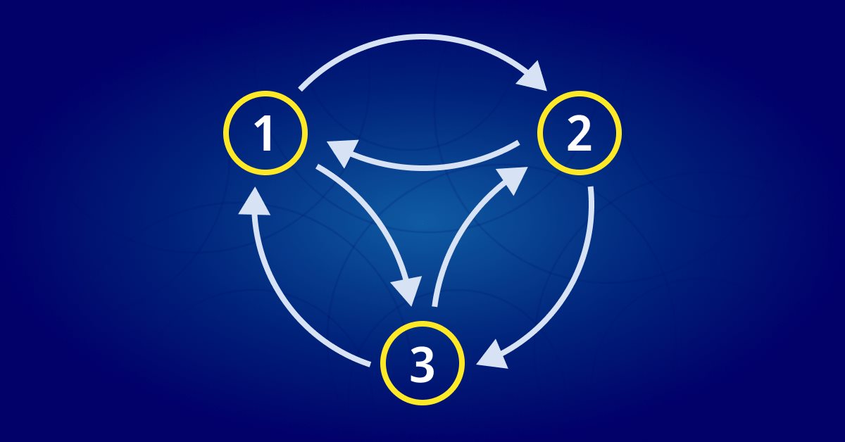
A Markov chain is a mathematical system that undergoes transitions from one state to another according to certain probabilistic rules. The defining characteristic of a Markov chain is that no matter how the system arrived at its current state, the probability of transitioning to any particular state is dependent solely on the current state and time elapsed. A Markov chain can be represented using a state diagram, where each node in the diagram represents a state and the edges between the nodes represent the transitions between the states. The probability of transitioning from one state to another is represented by the weight of the corresponding edge.

The arrows in the diagram (aka Markov chain) represent transitions between the states. The probability of transitioning from state 'rainy weather' to state 'sunny weather' can be represented by the weight of the edge between the two nodes (in this case 0.1), and similarly for the other transitions. 

We can use this state diagram to model the probabilities of transitioning between states in the system. The model we create is better referred to as a transition matrix and this is illustrated above.

One important assumption of a Markov chain is that the future behavior of the system depends only on the current state and time elapsed, and not on the past history of the system. This is known as the "memoryless" property of a Markov chain. This implies the probability of transitioning from one state to another is the same regardless of how many intermediate states the system may have passed through to reach its current state.

Markov chains can be used to model a wide variety of systems, including financial systems, weather systems, and biological systems. They are particularly useful for modeling systems that exhibit temporal dependencies, where the current state of the system depends on its past states, such as time series.

Markov chains are widely used to model time series data, which is a series of data points collected at regular intervals over time. Time series data can be found in many different fields, such as finance, economics, meteorology, and biology.

To use a Markov chain to model time series data, it is first necessary to define the states of the system and the transitions between them. The transition probabilities between states can be estimated from the data using techniques such as maximum likelihood estimation or expectation maximization. Once the transition probabilities have been estimated, the Markov chain can be used to make predictions about future states or events based on the current state and time elapsed.

There are several ways in which Markov chains can be used to model time series data:

1. Discrete-time Markov chain: A discrete-time Markov chain is a mathematical model used to describe the evolution of a discrete-time stochastic process over a series of time steps. It can be used to model a sequence of events or states in which the probability of transitioning to any given state at a given time depends only on the current state. 

Here are some examples of how a discrete-time Markov chain could be used to model daily events:

• Weather forecasting: A discrete-time Markov chain could be used to model the daily weather in a particular location. The states of the Markov chain could represent different weather conditions, such as sunny, cloudy, rainy, or snowy. The transition probabilities could be estimated from historical weather data, and the Markov chain could be used to make forecasts about the weather for the next day based on the current weather condition.
• Stock price movements: A discrete-time Markov chain could be used to model the daily movements of a particular stock price. The states of the Markov chain could represent different levels of price movement, such as up, down, or unchanged. The transition probabilities could be estimated from historical stock price data, and the Markov chain could be used to make forecasts about the direction of the stock price for the next day based on the current price movement.
• Traffic patterns: A discrete-time Markov chain could be used to model the daily traffic patterns on a particular road or highway. The states of the Markov chain could represent different levels of traffic congestion, such as light, medium, or heavy. The transition probabilities could be estimated from historical traffic data, and the Markov chain could be used to make forecasts about the level of traffic congestion for the next day based on the current level of congestion.

2. Continuous-time Markov chain:Here transitions between states occur continuously rather than at discrete time steps. This means that the probability of transitioning from one state to another depends on the time elapsed since the last transition. Continuous-time Markov chains are commonly used to model systems that change continuously over different spans of time, such as the flow of traffic on a particular highway or the rate of chemical reactions in a chemical plant. One of the main differences between discrete-time and continuous-time Markov chains is that the transition probabilities in a continuous-time Markov chain are characterised by transition rates, which are the probability of transitioning from one state to another per unit of time. These transition rates are used to compute the probability of transitioning from one state to another over a specific time interval.

3. Hidden Markov model: A hidden Markov model (HMM) is a statistical model is a type of Markov chain in which the states of the system are not directly observable, but are instead inferred from a sequence of observations. Here are some examples of how a hidden Markov model could be used to model common everyday events:

   • Speech recognition: A hidden Markov model could be used to model the sounds produced during speech and to recognize spoken words. In this case, the states of the HMM could represent different phonemes (speech sounds), and the observations could be a sequence of sound waves representing the spoken words. The HMM could be trained on a large dataset of spoken words and their corresponding sound waves, and could be used to recognize new spoken words by inferring the most likely sequence of phonemes based on the observed sound waves.
   • Handwriting recognition: A hidden Markov model could be used to model the sequence of pen strokes made during handwriting and to recognize handwritten words. In this case, the states of the HMM could represent different pen strokes, and the observations could be a sequence of images of handwritten words. The HMM could be trained on a large dataset of handwritten words and their corresponding images, and could be used to recognize new handwritten words by inferring the most likely sequence of pen strokes based on the observed images.
   • Activity recognition: A hidden Markov model could be used to recognize human activities based on a sequence of observations, such as sensor readings or video frames. For example, an HMM could be used to recognize activities such as walking, running, or jumping.

4. Markov switching model: A Markov switching model (MSM) is a type of Markov chain in which the states of the system can change over time, or "switch," based on certain conditions. Here are some examples of how a Markov-switching model could be used to model common everyday events:

   • Consumer behavior: A Markov-switching model could be used to model the purchasing behavior of consumers. The states of the MSM could represent different types of purchasing behavior, such as high-frequency purchasing or low-frequency purchasing. The transitions between states could be based on certain conditions, such as changes in income or the introduction of new products. The MSM could be used to forecast future purchasing behavior based on the current state and the transition probabilities between states.
   • Economic indicators: A Markov-switching model could be used to model economic indicators, such as GDP or unemployment rate. The states of the MSM could represent different economic conditions, such as expansion or recession, and the transitions between states could be based on certain conditions, such as changes in monetary policy or the business cycle. The MSM could be used to forecast future economic conditions based on the current state and the transition probabilities between states.
   • Traffic patterns: A Markov-switching model could be used to model the traffic patterns on a particular road or highway. The states of the MSM could represent different levels of traffic congestion, such as light, medium, or heavy, and the transitions between states could be based on certain conditions, such as the time of day or the day of the week. The MSM could be used to forecast future traffic patterns based on the current state and the transition probabilities between states.

   
   

As with any hypothesis, there are always underlying assumptions that tend to impose some form of limitation on the idea. Markov Chains are no exception, Here are some of the assumptions:

1. Stationarity: One of the main assumptions of a Markov chain is that the transition probabilities between states are constant over time. This assumption is known as stationarity. If the transition probabilities are not constant over time, the Markov chain model may not be accurate.

2. Markov property: Another assumption of a Markov chain is that the future evolution of the system is dependent only on the current state and time elapsed, and is not affected by the past history of the system beyond the current state. This assumption may not always hold in practice, particularly for data sets with complex dependencies or long-term memory.

3. Finite state space: A Markov chain is typically defined on a finite state space, which means that there is a finite number of possible states that the system can be in. This may not be suitable for data sets with a large number of states or continuous variables.

4. Time-homogeneity: A Markov chain is typically assumed to be time-homogeneous, which means that the transition probabilities between states do not depend on the specific time at which the transition occurs. If the transition probabilities do depend on the time at which the transition occurs, the Markov chain model may not be accurate.

5. Ergodicity: A Markov chain is typically assumed to be ergodic, which means that it is possible to reach any state from any other state in a finite number of steps. If this assumption is not met, the Markov chain model may not be accurate.

In general, Markov chain models are most appropriate for data sets with relatively simple dependencies and a small number of states or variables. If the data set has complex dependencies or a large number of states or variables, other modeling techniques may be more appropriate.

Probability Estimation

Once a Markov chain has been modelled we then need to estimate the probabilities of transitioning from each state. There are a number of methods that can be used and it will be helpful to iterate through them to get a better feel of the scope and possibilities of Markov Chains. There are several methods of estimating probabilities for transitioning between states in Markov chains, including:

1. Maximum likelihood estimation (MLE): In maximum likelihood probability estimation (MLE), the goal is to estimate the probability of an event or sequence of events based on observed data. In the context of Markov chains, this means that we want to estimate the probability of transitioning from one state to another based on a set of observed transitions.

   To implement MLE for Markov chains, we first need to collect a set of observed transitions. This can be done by running a simulation or by collecting real-world data. Once we have the observed transitions, we can use them to estimate the transition probabilities.

   To estimate the transition probabilities, we can use the following steps:

   • Define a matrix to store the transition probabilities. The matrix should have dimensions num_states x num_states , where num_states is the number of states in the Markov chain.
   • Initialize the matrix with all probabilities set to 0. This can be done using a nested loop that iterates over all elements of the matrix.
   • Iterate over the observed transitions and update the transition probabilities. For each observed transition from state i to state j , increment the probability transition_probs[i][j] by 1.
   • Normalize the transition probabilities so that they sum to 1. This can be done by dividing each element in the matrix by the sum of the elements in the corresponding row.

   
   

   Once the transition probabilities have been estimated, we can use them to predict the likelihood of transitioning from one state to another. For example, if we want to predict the probability of transitioning from state i to state j , we can use the formula P(j | i) = transition_probs[i][j] .

   .
2. Bayesian estimation: This method involves using Bayes' theorem to update the probability distribution over the model parameters based on new data. To use Bayesian probability estimation with a Markov chain, we first need to define a prior distribution over the states of the Markov chain. This prior distribution represents our initial belief about the probabilities of the different states in the chain. We can then use Bayesian updating to update our beliefs about the probabilities of the states as new information becomes available. For example, suppose we have a Markov chain with three states: A, B, and C. We start with a prior distribution over the states, which might be represented as:

   P(A) = 0.4 P(B) = 0.3 P(C) = 0.3

   This means that, initially, we believe that the probability of being in state A is 40%, the probability of being in state B is 30%, and the probability of being in state C is 30%.

   Now suppose we observe that the system transitions from state A to state B. We can use this new information to update our beliefs about the probabilities of the states using Bayesian probability estimation. To do this, we need to know the transition probabilities between the states. Let's suppose that the transition probabilities are as follows:

   P(A -> B) = 0.8 

   P(A -> C) = 0.2 

   P(B -> A) = 0.1 

   P(B -> B) = 0.7 

   P(B -> C) = 0.2 

   P(C -> A) = 0.2 

   P(C -> B) = 0.3 

   P(C -> C) = 0.5

   These transition probabilities tell us the probability of transitioning from one state to another. For example, the probability of transitioning from state A to state B is 0.8, while the probability of transitioning from state A to state C is 0.2.

   Using these transition probabilities, we can now update our beliefs about the probabilities of the states using Bayesian probability estimation. In particular, we can use Bayes' rule to compute the posterior distribution over the states given the new information that the system transitioned from state A to state B. This posterior distribution represents our updated belief about the probabilities of the states, taking into account the new information we have received.

   For example, using Bayes' rule, we can compute the posterior probability of being in state A as follows:

   P(A | A -> B) = P(A -> B | A) * P(A) / P(A -> B)

   Plugging in the values from our prior distribution and the transition probabilities, we get:

   P(A | A -> B) = (0.8 * 0.4) / (0.8 * 0.4 + 0.1 * 0.3 + 0.2 * 0.3) = 0.36

   Similarly, we can compute the posterior probabilities of being in states B and C as:

   P(B | A -> B) = (0.1 * 0.3) / (0.8 * 0.4 + 0.1 * 0.3 + 0.2 * 0.3) = 0.09

   .
3. Expectation-maximization (EM) algorithm: To use EM for probability estimation with a Markov chain, you would need to observe the transitions between states of the Markov chain over a period of time. From this data, you could use the EM algorithm to estimate the transition probabilities by iteratively refining your estimates based on the observed data. The EM algorithm works by alternating between two steps: the expectation step (E-step) and the maximization step (M-step). In the E-step, you estimate the expected value of the complete data log-likelihood, given the current estimates of the parameters. In the M-step, you maximize the expected value of the complete data log-likelihood with respect to the parameters, to obtain updated estimates of the parameters. You then repeat these steps until the estimates of the parameters converge to a stable value. For example, if you observed a Markov chain with three states (A, B, and C) and wanted to estimate the transition probabilities between the states, you could use the EM algorithm to iteratively refine your estimates of the transition probabilities based on the observed data.

   The main advantage of using EM for probability estimation is that it can handle incomplete or noisy data and can estimate the parameters of a statistical model even when the underlying distribution is not fully known. However, EM can be sensitive to initialization and may not always converge to the global maximum of the log-likelihood function. It can also be computationally intensive, as it requires repeatedly evaluating the log-likelihood function and its gradient.

4. Parametric estimation: To use parametric probability estimation with a Markov chain, you would need to observe the transitions between states of the Markov chain over a period of time. From this data, you could fit a parametric model to the transition probabilities by assuming that the underlying distribution follows a particular distribution, such as a normal distribution or a binomial distribution. You would then use this model to estimate the probability of transitioning from one state to another. For example, if you observed a Markov chain with three states (A, B, and C) and found that the transition from state A to state B occurred 10 times out of a total of 20 transitions, you could fit a binomial model to the data and use it to estimate the probability of transitioning from state A to state B.

   The main advantage of parametric probability estimation is that it can be more accurate than non-parametric methods, which do not make any assumptions about the underlying distribution. However, it requires making assumptions about the underlying distribution, which may not always be appropriate or may lead to biased estimates. Additionally, parametric methods can be less flexible and less robust than non-parametric methods, as they are sensitive to deviations from the assumed distribution.

5. Nonparametric estimation: To use non-parametric probability estimation with a Markov chain, you would need to observe the transitions between states of the Markov chain over a period of time. From this data, you could estimate the probability of transitioning from one state to another by counting the number of times the transition occurred and dividing it by the total number of transitions. For example, if you observed a Markov chain with three states (A, B, and C) and found that the transition from state A to state B occurred 10 times out of a total of 20 transitions, you could estimate the probability of transitioning from state A to state B as 0.5.

   This method of probability estimation is called the empirical distribution method, and it can be used to estimate the probabilities of any set of events, not just transitions in a Markov chain. The main advantage of non-parametric probability estimation is that it does not require any assumptions about the underlying distribution, making it a flexible and robust method for estimating probabilities. However, it can be less accurate than parametric methods, which make assumptions about the underlying distribution in order to estimate probabilities more precisely.

6. Bootstrapping: This is a general technique that can be used to estimate probabilities in a Markov chain, or in any other probabilistic model. The basic idea is to use a small number of observations to estimate the probability distribution over the states of the system, and then use that distribution to generate a large number of synthetic observations. The synthetic observations can then be used to estimate the probability distribution more accurately, and the process can be repeated until the desired level of accuracy is achieved.

   To use bootstrapping for probability estimation in a Markov chain, you would first need to have an initial Markov chain with its states. Like the Bayesian method, bootstrapping updates and improves existing Markov Chains. Each state in the chain is associated with a probability of transitioning to other states, and the probabilities of transitioning between different pairs of states are independent of the history of the system. Once you have the initial Markov chain, you can use bootstrapping to estimate the probability distribution over its states. To do this, you would start with a small number of observations of the system, such as a few initial state configurations or a short sequence of transitions between states. You can then use these observations to estimate the probability distribution over the states of the system.

   For example, if you have a Markov chain with three states A, B, and C, and you have observed the system transitioning from state A to state B a few times and from state B to state C a few times, you can use these observations to estimate the probability of transitioning from state A to state B and from state B to state C.

   Once you have estimated the probability distribution over the states of the system, you can use it to generate a large number of synthetic observations of the system. This can be done by randomly sampling from the probability distribution to simulate transitions between states. You can then use the synthetic observations to estimate the probability distribution more accurately, and repeat the process until you have achieved the desired level of accuracy.

   Bootstrapping can be a useful technique for estimating probabilities in a Markov chain because it allows you to use a small number of observations to generate a large number of synthetic observations, which can increase the accuracy of your estimates. It is also relatively simple to implement and can be used with a wide range of probabilistic models. However, it is important to note that the accuracy of the estimates obtained using bootstrapping will depend on the quality of the initial observations and the underlying probabilistic model, and may not always be as accurate as other estimation techniques.

7. Jackknife estimation: This method involves running multiple simulations of the Markov chain, each time leaving out a different state or group of states. The probability of the event occurring is then estimated by averaging the probabilities of the event occurring in each of the simulations. Here is a more detailed explanation of the process:
   • Set up the Markov chain and define the event of interest. For example, the event might be reaching a certain state in the chain, or transitioning between two specific states.
   • Run multiple simulations of the Markov chain, each time leaving out a different state or group of states. This can be done by simply not considering the excluded states when running the simulation, or by setting their transition probabilities to zero.
   • For each simulation, calculate the probability of the event occurring. This can be done by performing a detailed balance analysis, or by using techniques such as Monte Carlo sampling or matrix multiplication.
   • Average the probabilities of the event occurring in each of the simulations to obtain an estimate of the probability of the event occurring in the full Markov chain.

   There are several advantages to using the jackknife method for probability estimation in Markov chains. One advantage is that it allows for a more accurate estimate of the probability of the event occurring, as it takes into account the effect of each individual state on the overall probability. Another advantage is that it is relatively simple to implement and can be easily automated. However, there are also some limitations to the jackknife method. One limitation is that it requires running multiple simulations of the Markov chain, which can be computationally intensive for large or complex chains. Additionally, the accuracy of the estimate may depend on the number and choice of states that are excluded in the simulations.

8. Cross-validation: This method can be used to estimate the probability of a particular event occurring within a Markov chain. It involves dividing the data into a number of folds, or subsets, and using each fold as a test set to evaluate the model's performance on that subset. To use cross-validation probability estimation with Markov chains, we would first need to set up the Markov chain with the desired states and transitions. Then, we would divide the data into the desired number of folds. Next, we would iterate through each fold and use it as a test set to evaluate the model's performance on that subset. This would involve using the Markov chain to estimate the probability of each event occurring within the test set, and comparing these estimates to the actual outcomes in the test set.

   Finally, we would average the performance across all of the folds to get an overall estimate of the model's performance. This can be useful for evaluating the performance of the model and fine-tuning the parameters of the Markov chain to improve its accuracy. It's important to note that in order to use cross-validation probability estimation with a Markov chain, the data must be independently and identically distributed, meaning that each subset of data should be representative of the overall dataset.

Each of these methods has its own strengths and limitations, and the choice of method will depend on the specific characteristics of the data and the goals of the analysis. 

Implementation with MQL5 Wizard

To code a signal class that implements Markov Chains we will use the 'CMarkovCPD' class in the 'dataanalysis.mqh' file under 'alglib' folder. So we'll model the chains as discrete-time chains. These discrete-time chain will have 5 states that are simply the last 5 changes in close price. So the timeframe on which the expert is tested or run will define the discrete time unit. In order to estimate the probabilities of transitioning between states the 'CMarkovCPD' class requires tracks are added in order to train the model. The number of added tracks will be an input optimisable parameter 'm_signal_tracks'. This is how we would initialise the mode and add the tracks (training data).

      CMCPDState _s;
      CMatrixDouble _xy,_p;
      CMCPDReport _rep;
      int _k=m_signal_tracks;
      
      _xy.Resize(m_signal_tracks,__S_STATES);
      
      m_close.Refresh(-1);
      
      for(int t=0;t<m_signal_tracks;t++)
      {
         for(int s=0;s<__S_STATES;s++)
         {
            _xy[t].Set(s,GetState(Close(Index+t+s)-Close(Index+t+s+1),Close(Index+t+s+1)-Close(Index+t+s+2)));
         }
      }

The close price data is normalised about 1.0. If the change in close is negative the input data is less than 1.0, if on the other hand it is positive, the input will be more than 1.0 with no changes giving exactly 1.0. This normalisation is accomplished by the 'GetState' function shown below.

//+------------------------------------------------------------------+
//| Normalizer.                                                      |
//+------------------------------------------------------------------+
double CSignalMC::GetState(double NewChange,double OldChange)
   {
      double _state=0.0;
      
      double _norm=fabs(NewChange)/fmax(m_symbol.Point(),fabs(NewChange)+fabs(OldChange));
      
      if(NewChange>0.0)
      {
         _state=_norm+1.0;
      }
      else if(NewChange<0.0)
      {
         _state=1.0-_norm;
      }
      
      return(_state);
   }

Once we've added our data we then need to initialise an instance of 'CMCPDState' class as this is the object that handles all our model data and aids in calculating probability estimates. We do this as so:

      CPD.MCPDCreate(__S_STATES,_s);
      
      CPD.MCPDAddTrack(_s,_xy,_k);
      
      CPD.MCPDSetTikhonovRegularizer(_s,m_signal_regulizer);
      
      CPD.MCPDSolve(_s);
      
      CPD.MCPDResults(_s,_p,_rep);

The 'm_signal_regulazier' input parameter should ideally not be an abstract double value but a double value that is representative of the magnitude of the track data. In other words it should be proportional to the track data as got from the 'GetState' function. This means if you ideally optimise it to say between the range 0.5-0.0, you should multiply it by the magnitude of the largest track data when using the Tikhonov regulizer. 

The '_p' matrix is our transition matrix with all the probabilities of transitioning between states. Full code of the signal class is attached at the end of the article.

I made some test runs on EURJPY for 2022 on the daily time frame and below is part of the report and the attendant equity curve.

Conclusion

Markov chains are a mathematical tool that can be used to model the behavior of financial markets. They are particularly useful because they allow traders to analyze the probability of future market states based on the current state of the market. This can be very useful in trading, as it allows traders to make informed decisions about which trades to make and when to make them.

One of the key benefits of using Markov chains in financial markets is that they allow traders to analyze and predict the evolution of market trends over time. This is especially important in fast-moving markets, where trends can change rapidly and it is difficult to predict how the market will behave. By using Markov chains, traders can identify the most likely paths that the market will take and use this information to make informed trading decisions.

Another benefit of Markov chains is that they can be used to analyze the risk associated with different trades. By analyzing the probabilities of different market states, traders can determine the risk associated with different trades and choose trades that are most likely to be successful. This can be especially useful in volatile markets, where the risk of loss is higher.

In conclusion, Markov chains are an essential tool for traders in financial markets because they allow traders to analyze and predict the behavior of the market, identify the most likely paths that the market will take, and assess the risk associated with different trades.