Data Science and Machine Learning (Part 10): Ridge Regression

Introduction 

Ridge regression is the method of estimating the coefficients of multiple-regression models in scenarios where the independent variables are highly correlated. The method provides improved efficiency in parameters estimation problems in exchange for a tolerable amount of bias meanwhile Lasso (Least absolute shrinkage and selection operator) is a regression analysis method that performs both variable selection and regularization to enhance the prediction accuracy and interpretability of the resulting statistical model. Lasso was originally formulated for linear regression models. This simple case reveals a substantial amount about the estimator. These include its relationship to ridge regression and best subset selection and the connections between lasso coefficient estimates and so-called soft thresholding. It also reveals that (like standard linear regression) the coefficient estimates do not need to be unique if covariates are collinear.

Now to understand why we need such models in the first place let's understand the term bias and variance.

Bias 

is the inability of machine learning to capture the true relationship between the independent and response variable

What does this mean to the model?

• Low bias: The model with a low bias makes fewer assumptions about the form of the target function
• High bias: The model with a high bias makes more assumptions and can capture relationships within the training dataset

Variance

Variance tells how much a random variable is different from its expected value.
Ways to reduce High Bias.

• Increase the input features as the model is under fitted
• Decrease the regularization term
• Use more complex features such as including some polynomial features

Ways to reduce High Variance.

• Reduce the input features; The number of parameters as the model is under fitted
• Do not use much complex model
• Increase the training data
• Increase the regularization term

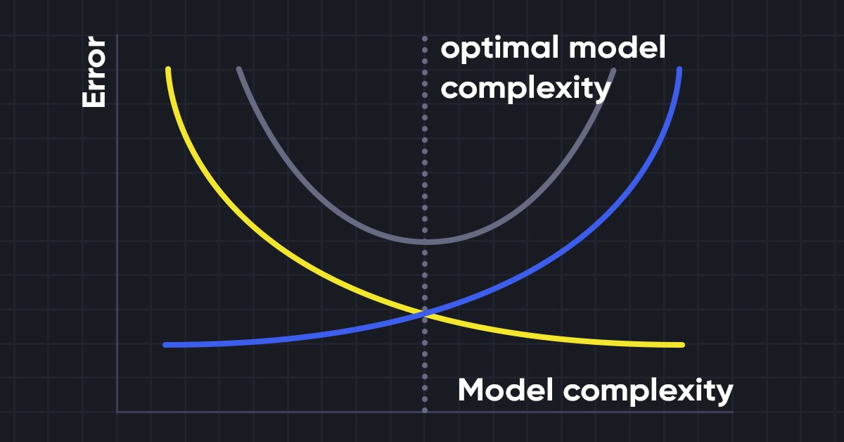
Bias-Variance Trade-off

While building the machine learning model it is really important to take care of bias and variance to avoid overfitting the model. If the model is very simple and with fewer parameters, it tends to have more bias but small variance, whereas the complex models oftentimes end up having low bias yet high variance value. so it is required to make a balance between bias and variance errors, Finding the balance between these two terms is known as the bias-variance tradeoff.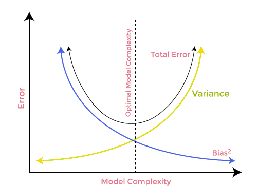
For accurate predictions of the model, algorithms need a lower bias and lower variance as well but this is practically impossible because bias and variance are negatively related to each other.

If we increase the bias, the variance will decrease and vice-versa is true

Ridge regression

Ridge and lasso regression both are on the same mission yet they have a major difference that we will see later on, when diving into the math's and trying to figure out what makes each algorithm tick.

The idea behind ridge regression.

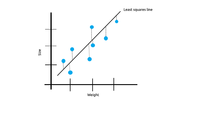
When we have a lot of measurements that are linearly correlated we can be confident that the least squares will do just fine work of reflecting the relationship between the independent variable and the target variable.

Take a look at the below example of mice sizes plotted against mice weight.

But, what if only have two measurements as our training dataset and the rest as our testing dataset, Fitting the model with the least square will result in a perfect fit that gives us a zero-sum of squared residuals.

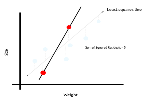
Now let's test this model on a new dataset;

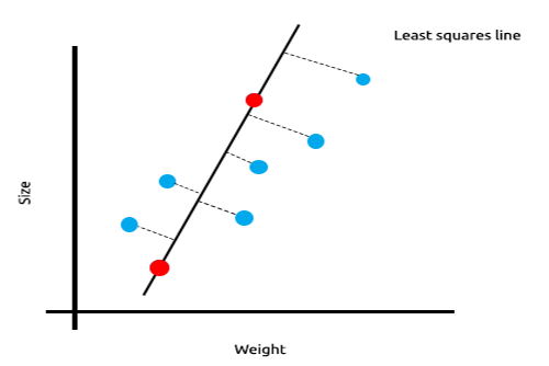
The sum of squared errors for the training data is zero but the sum of the squared residuals for the testing data is large, this means that our model has high variance, In machine learning lingo we say that this model is overfit to the training data.

The main idea behind ridge and lasso regression is to find the model that doesn't fit the training data as well.

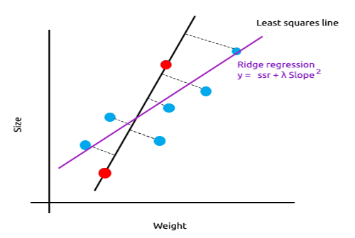
In ridge regression, a small amount of bias is introduced into the new line by introducing a small amount of bias, we get a significant drop in variance. Since the ridge regression has introduced a small amount of bias the model now doesn't fit well both the training data and the testing data provide us with a reliable model in the long term.

When to use these regularized models.

One may ask themselves if a least squares method/the Linear regression model can do just well why use this L1norm and L2Norm models?

To understand this let's see how a multivariable linear regression performs on the trained dataset

To illustrate well the point I'm trying to make I have prepared the dataset full of oscillators and the volume indicator for EURUSD;

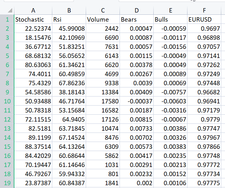
Without even looking at the correlation matrix every one who is familiar with these indicators knows for sure that these indicators are not suitable for regression problems. Below is the Correlation matrix

    ArrayPrint(matrix_utils.csv_header);
    Print(Matrix.CorrCoef(false));

Result:

CS      0       06:29:41.493    TestEA (EURUSD,H1)      "Stochastic" "Rsi"        "Volume"     "Bears"      "Bulls"      "EURUSD"    
CS      0       06:29:41.493    TestEA (EURUSD,H1)      [[1,0.680705511991766,0.02399740959375265,0.6910892641498844,0.7291018045506749,0.1490856367010467]
CS      0       06:29:41.493    TestEA (EURUSD,H1)       [0.680705511991766,1,0.07620207894739518,0.8184961346648213,0.8258569040865805,0.1567269000583347]
CS      0       06:29:41.493    TestEA (EURUSD,H1)       [0.02399740959375265,0.07620207894739518,1,0.3752014290536041,-0.1289026185114097,-0.1024017077869821]
CS      0       06:29:41.493    TestEA (EURUSD,H1)       [0.6910892641498844,0.8184961346648213,0.3752014290536041,1,0.7826404088603456,0.07283638913665436]
CS      0       06:29:41.493    TestEA (EURUSD,H1)       [0.7291018045506749,0.8258569040865805,-0.1289026185114097,0.7826404088603456,1,0.08392530400705019]
CS      0       06:29:41.493    TestEA (EURUSD,H1)       [0.1490856367010467,0.1567269000583347,-0.1024017077869821,0.07283638913665436,0.08392530400705019,1]]

As you can see the Correlations are less than 20% for the EURUSD column against all the indicators, The stochastic indicator and the RSI seems to be best correlated than the others but only for about 14 and 15 percent respectively. Let's create a linear regression model starting with the stochastic indicator only then we will keep on adding the independent variables/ other indicators readings.

Table of Results:

Independent Variables	R2 Score(Accuracy)
Stochastic	1.2 %
Stochastic and RSI	1.8 %
Stochastic, RSI and Volume	2.8 %
Stochastic, RSI, Volume, Bears Power, and Bulls Power   (All independent variables)	4.9%

So what conclusion can you draw from this table; As you increase the number of independent variables the accuracy of the trained linear model always increases regardless of what are those variables, The correlation for the independent variables I have used in this example is very low that's why you see a slight improvement in accuracy each time a new independent variable is added but that might not be the case when the variables are correlated for about 30% to 40% each you may witness your model get up to an accuracy of 90% in the training phase when you give it too many of those independent variables.

The increase of independent variables increases the variance, it is no doubt that this model will perform worse in the new dataset since it is overfitting, To solve this issue both ridge and lasso regression were introduced, as said earlier by adding some kind of bias we get a significant drop in variance.

Ridge Regression Theory

Ridge regression itself is a method of estimating the coefficients of a linear regression model when the independent variables are highly correlated.

Ridge regression was developed as a possible solution to the imprecision of least square estimators when the linear regression models have some multicollinear(highly correlated) -- by creating a ridge regression estimator(RR). This provides more precise ridge parameters as its variance and bias are often smaller than the least square estimators.

Ridge estimator

Analogous to the ordinary least squares estimator, the simple ridge estimator is given by 

where y is the independent variable matrix, X is the design matrix, I is the identity matrix and the ridge parameter λ is the value greater than or equal to zero.

Let's write code for this:

CRidgeregression::CRidgeregression(matrix &_matrix)
 {
    
    n = _matrix.Rows();
    k = _matrix.Cols();
    
    pre_processing.Standardization(_matrix);
    m_dataset.Copy(_matrix);
    
    matrix_utils.XandYSplitMatrices(_matrix,XMatrix,yVector);
    
    YMatrix = matrix_utils.VectorToMatrix(yVector);
    
//---

    Id_matrix.Resize(k,k);
    
    Id_matrix.Identity();

 }

On the function constructor, three important things get done, First is Standardizing the data. Just like the multivariable gradient descent and many other machine learning techniques, The ridge regression works in the standardized dataset, Second the data is split into x and y matrices, and lastly the Identity matrix gets created.

Inside the L2Norm Function:

vector CRidgeregression::L2Norm(double lambda)
 {    
   matrix design = matrix_utils.DesignMatrix(XMatrix);
   
   matrix XT = design.Transpose();
   
   matrix XTX = XT.MatMul(design);
   
   matrix lamdaxI = lambda * Id_matrix;
   
   //Print("LambdaxI \n",lamdaxI);
   
   //Print("XTX\n",XTX);
   
   matrix sum_matrix = XTX + lamdaxI;
   
   matrix Inverse_sum = sum_matrix.Inv();
   
   matrix XTy = XT.MatMul(YMatrix);
   
   Betas = Inverse_sum.MatMul(XTy);
 
   #ifdef DEBUG_MODE
      Print("Betas\n",Betas);
   #endif 
   
  return(matrix_utils.MatrixToVector(Betas));
 } 

This function does everything as instructed by the above formula we just saw for finding the coefficients using the Ridge regression.

To see how this works let's use another dataset NASDAQ_DATA.csv that the reader of this Article series are already familiar with.

int OnInit()
  {
//---
    matrix Matrix = matrix_utils.ReadCsv("NASDAQ_DATA.csv",","); 
   
    pre_processing.Standardization(Matrix);
    Linear_reg = new  CLinearRegression(Matrix);
    
    ridge_reg = new CRidgeregression(Matrix);
    
    ridge_reg.L2Norm(0.3);
 }    

I have set the random penalty value of 0.3 for the ridge regression just so that we can see what comes out of this. Now it's time to run the function and see what coefficients come out of this;

CS 0 10:27:41.338 TestEA (EURUSD,H1) [[5.015577002384403e-16]

CS 0 10:27:41.338 TestEA (EURUSD,H1) [0.6013523727380532]

CS 0 10:27:41.338 TestEA (EURUSD,H1) [0.3381524618200134]

CS 0 10:27:41.338 TestEA (EURUSD,H1) [0.2119467984461254]]

Let's also run the Linear regression model for the same dataset and observe their coefficients too, Since the Least squares method doesn't standardize the dataset, Let's also standardize it before giving the data to the model.

    matrix Matrix = matrix_utils.ReadCsv("NASDAQ_DATA.csv",","); 
   
    pre_processing.Standardization(Matrix);
    Linear_reg = new  CLinearRegression(Matrix);

Output:

CS 0 10:27:41.338 TestEA (EURUSD,H1) Betas

CS 0 10:27:41.338 TestEA (EURUSD,H1) [[-4.143037461930866e-14]

CS 0 10:27:41.338 TestEA (EURUSD,H1) [0.6034777119810752]

CS 0 10:27:41.338 TestEA (EURUSD,H1) [0.3363532376334173]

CS 0 10:27:41.338 TestEA (EURUSD,H1) [0.21126507562567]]

The coefficients look slightly different so I guess our function works let's train and test each of the models then finally plot their respective graphs to understand more.

Since the ridge regression itself is not a model is an estimator for the coefficients which need to then be used with the linear regression model, I made some changes to the Linear regression class we  discussed in part 3. 

In Linear regression class constructor is where the model gets trained. It is an area where the coefficients are then stored to be used by the rest of the functions, I have added a new constructor that allows passing the coefficients to the model, This will help us do the minimum effort the next time we use other estimators to get the coefficients that we want our regression model to use.

class CLinearRegression
  {
   public: 
                        CLinearRegression(matrix &Matrix_); //Least squares estimator
                        CLinearRegression(matrix<double> &Matrix_, double Lr, uint iters = 1000); //Lr by Gradient descent
                        CLinearRegression(matrix &Matrix_, vector &coeff_vector);
                        
                       ~CLinearRegression(void);

Ridge vs Linear Regression

    Print("----> Ridge regression");
    
    ridge_reg = new CRidgeregression(Matrix);
    vector coeff = ridge_reg.L2Norm(0.3);
    
    Linear_reg = new CLinearRegression(Matrix,coeff); //passing the coefficients made by ridge regression
                                                      // to the Linear regression model
    double acc =0;
    
    vector ridge_predictions = Linear_reg.LRModelPred(Matrix,acc); //making the predictions and storing them to a vector
    
    delete(Linear_reg); //deleting that instance
    
    Print("----> Linear Regression");
   
    pre_processing.Standardization(Matrix);
     
    Linear_reg = new CLinearRegression(Matrix); //new Linear reg instance that gets coefficients by least squares
    
    vector linear_pred = Linear_reg.LRModelPred(Matrix,acc); 

Outputs:

CS 0 11:35:52.153 TestEA (EURUSD,H1) ----> Ridge regression

CS 0 11:35:52.153 TestEA (EURUSD,H1) Betas

CS 0 11:35:52.153 TestEA (EURUSD,H1) [[-4.142058558619502e-14]

CS 0 11:35:52.153 TestEA (EURUSD,H1) [0.601352372738047]

CS 0 11:35:52.153 TestEA (EURUSD,H1) [0.3381524618200102]

CS 0 11:35:52.153 TestEA (EURUSD,H1) [0.2119467984461223]]

CS 0 11:35:52.154 TestEA (EURUSD,H1) R squared 0.982949 Adjusted R 0.982926

CS 0 11:35:52.154 TestEA (EURUSD,H1) ----> Linear Regression

CS 0 11:35:52.154 TestEA (EURUSD,H1) Betas

CS 0 11:35:52.154 TestEA (EURUSD,H1) [[5.014846059117108e-16]

CS 0 11:35:52.154 TestEA (EURUSD,H1) [0.6034777119810601]

CS 0 11:35:52.154 TestEA (EURUSD,H1) [0.3363532376334217]

CS 0 11:35:52.154 TestEA (EURUSD,H1) [0.2112650756256718]]

CS 0 11:35:52.154 TestEA (EURUSD,H1) R squared 0.982933 Adjusted R 0.982910

The models have a slightly different performance when you use all the data as the training data.

When the outputs were stored and plotted in the same axis this is their graph;

I can hardly see any difference between the Linear model to the predictor marked in blue, I can only see the difference between the two models and the ridge regression doesn't fit well to the dataset, that's good news. Let's train and test both of the models one by one.

    matrix_utils.TrainTestSplitMatrices(Matrix,TrainMatrix,TestMatrix);
    
    Print("----> Ridge regression | Train ");
    
    ridge_reg = new CRidgeregression(TrainMatrix);
    vector coeff = ridge_reg.L2Norm(0.3);
    
    Linear_reg = new CLinearRegression(TrainMatrix,coeff); //passing the coefficients made by ridge regression
                                                      // to the Linear regression model
    Linear_reg.LRModelPred(TrainMatrix,acc);
    
    printf("Accuracy %.5f ",acc);
    
    Print("----> Ridge regression | Test");
    
    vector ridge_predictions = Linear_reg.LRModelPred(TestMatrix,acc); //making the predictions and storing them to a vector
    
    printf("Accuracy %.5f ",acc);
    
    delete(Linear_reg); //deleting that instance
    
    Print("\n----> Linear Regression | Train ");
     
    Linear_reg = new CLinearRegression(TrainMatrix); //new Linear reg instance that gets coefficients by least squares
    
    Linear_reg.LRModelPred(TrainMatrix,acc);
    
    printf("Accuracy %.5f ",acc);
    
    Print("----> Linear Regression | Test ");
    
    vector linear_pred = Linear_reg.LRModelPred(TestMatrix,acc); 
    
    printf("Accuracy %.5f ",acc);
    

Output:

CS 0 13:27:40.744 TestEA (EURUSD,H1) ----> Ridge regression | Train 

CS 0 13:27:40.744 TestEA (EURUSD,H1) Accuracy 0.97580 

CS 0 13:27:40.744 TestEA (EURUSD,H1) ----> Ridge regression | Test

CS 0 13:27:40.744 TestEA (EURUSD,H1) Accuracy 0.78620 

CS 0 13:27:40.744 TestEA (EURUSD,H1)

CS 0 13:27:40.744 TestEA (EURUSD,H1) ----> Linear Regression | Train 

CS 0 13:27:40.744 TestEA (EURUSD,H1) Accuracy 0.97580 

CS 0 13:27:40.744 TestEA (EURUSD,H1) ----> Linear Regression | Test 

CS 0 13:27:40.744 TestEA (EURUSD,H1) Accuracy 0.78540 

It appears that both of the models had approximately the same accuracy in training but a slight difference in the testing dataset, not bad considering the penalty that the ridge regression uses to punish the independent variables 0.3 is small and we are yet to figure out how to choose the right penalty.

When I set the lambda value to 10 the ridge regression training accuracy dropped to 0.95760 from 0.97580 while the testing accuracy rose from 0.78540 to 0.80050 small increase of course.

Choosing the right penalty value(lambda)

To find the right values of lambda we need to use the LEAVE ONE OUT CROSS VALIDATION(LOOCV) technique, for those who are not familiar with it, this is the technique to find the optimal parameters of some of the models in ML the way it achieves this is going through all the dataset leaving I sample out of the dataset then trains the model with the rest of the dataset which is n-1 then uses the one sample that was left out as the testing sample, it goes through all the dataset up to nth samples, it finally measures the loss for all the values in each iteration finally it finds where was the minimal loss function at specific values of lambda, the one that produces the least error, is the best parameter, for more info read.

Let's import the cross-validation class to help us find the optimal value of the lambda.

#include <MALE5\cross_validation.mqh>
CCrossValidation *cross_validation;

Below is the code for LOOCV for Ridge regression;

double CCrossValidation::LeaveOneOut(double init, double step, double finale)
 {
    matrix XMatrix;
    vector yVector;
    
    matrix_utils.XandYSplitMatrices(Matrix,XMatrix,yVector);
 
    matrix train = Matrix; vector test = {};
    
    int size = int(finale/step);
    vector validation_output(ulong(size));
    vector lambda_vector(ulong(size));
    
    vector forecast(n); 
    vector actual = yVector;
    
    double lambda = init;
    
     for (int i=0; i<size; i++)
       {
         lambda += step;
         
          for (ulong j=0; j<n; j++)
            {               
               train.Copy(Matrix);
               ZeroMemory(test);
               
               test = XMatrix.Row(j);
               
               matrix_utils.MatrixRemoveRow(train,j);
               
               vector coeff = {};
               double acc =0;
               
                switch(selected_model)
                  {
                   case  RIDGE_REGRESSION:

                        ridge_regression = new CRidgeregression(train);
                        coeff = ridge_regression.L2Norm(lambda); //ridge regression
                        
                        Linear_reg = new CLinearRegression(train,coeff);   

                        forecast[j] =  Linear_reg.LRModelPred(test);  
                        
                        //---
                        
                        delete (Linear_reg); 
                        delete (ridge_regression);
                        
                     break; 
                  }
            }
          
          validation_output[i] = forecast.Loss(actual,LOSS_MSE)/double(n); 
          
          lambda_vector[i] = lambda;
          
          #ifdef DEBUG_MODE
             printf("%.5f LOOCV mse %.5f",lambda_vector[i],validation_output[i]);
          #endif           
       }

//---

      #ifdef  DEBUG_MODE
         matrix store_matrix(size,2);
         
         store_matrix.Col(validation_output,0);
         store_matrix.Col(lambda_vector,1); 
         
         string name = EnumToString(selected_model)+"\\LOOCV.csv";
         
         string header[2] = {"Validation output","lambda"};
         matrix_utils.WriteCsv(name,store_matrix,header);
      #endif 
      
    return(lambda_vector[validation_output.ArgMin()]);
 }

Let's put this into action;

int OnInit()
  {    
    matrix Matrix = matrix_utils.ReadCsv("NASDAQ_DATA.csv",",");  
    
    ridge_reg = new CRidgeregression(Matrix);
    
    cross_validation = new CCrossValidation(Matrix,RIDGE_REGRESSION);
    
    double best_lambda = cross_validation.LeaveOneOut(0,1,10);
    
    Print("Best lambda ",best_lambda);

Output:

CS      0       10:12:51.346    ridge_test (EURUSD,H1)  1.00000 LOOCV mse 0.00020
CS      0       10:12:51.465    ridge_test (EURUSD,H1)  2.00000 LOOCV mse 0.00020
CS      0       10:12:51.576    ridge_test (EURUSD,H1)  3.00000 LOOCV mse 0.00020
CS      0       10:12:51.684    ridge_test (EURUSD,H1)  4.00000 LOOCV mse 0.00020
CS      0       10:12:51.788    ridge_test (EURUSD,H1)  5.00000 LOOCV mse 0.00020
CS      0       10:12:51.888    ridge_test (EURUSD,H1)  6.00000 LOOCV mse 0.00020
CS      0       10:12:51.987    ridge_test (EURUSD,H1)  7.00000 LOOCV mse 0.00021
CS      0       10:12:52.090    ridge_test (EURUSD,H1)  8.00000 LOOCV mse 0.00021
CS      0       10:12:52.201    ridge_test (EURUSD,H1)  9.00000 LOOCV mse 0.00021
CS      0       10:12:52.317    ridge_test (EURUSD,H1)  10.00000 LOOCV mse 0.00021
CS      0       10:12:52.319    ridge_test (EURUSD,H1)  Best lambda 1.0

Assuming there are no bugs in the code, the best value of lambda is one when the search was from 1 to 10. This tells us that the value of lambda for this model is somewhat smaller so I decided to run the loop from 0 to 10 the step size was set to 0.01 (total 1000 iterations), it did take like 5 minutes to complete but, I was able to obtain the value of 0.09 as the best value of lambda, Below is the plot;

Cool, Now everything is just fine on the ridge regression part.

Advantages of Ridge Regression

• let's see some benefits of using a ridge regression estimator
•  It protects the model from overfitting
•  Model complexity is reduced
•  it performs well that the linear regression in the multivariable dataset
•  it doesn't need unbiased estimators

Disadvantages of ridge regression

•  it includes all the predictors in the final model
•  It is not capable of performing feature selection
•  It shrinks coefficients toward zero
•  it trades variance for bias

Final thoughts

The ridge regression may help to avoid overfitting the regression model in cases where there are multivariable but, it is still crucial to avoid/remove unwanted variables yourself manually from the model, from our NASDAQ_DATA we could have removed the RSI column because all of us we probably know that it's not correlated to our target variable, That's it for this article there is so much stuff going on that I can't cover for now.

Keep tracking the ridge regression development on my GitHub repo > https://github.com/MegaJoctan/MALE5

Filename	Description
cross_validation.mqh	Just like sklearn cross validation, This file contains validation techniques such as LOOCV
Linear regression.mqh	This file contains the least square method/ The Linear regression model
matrix_utils.mqh	This utility class function contains extra matrix operations functions
Preprocessing.mqh	Just like sklearn.preprocessing, This class contains functions that can be used to manipulate and rescale datasets
Ridge Regression.mqh	This file contains the ridge regression model and its relevant functions
ridge_test.mq5	This is a script that is used to test everything we discussed in this article
prepare_dataset.mq5	This script creates a dataset for the oscillators indicators that we discussed previously. This data will be stored into a file   Oscillators.csv
NASDAQ_DATA.csv	This csv file contains the dataset we have used in this article