Building a Profitable Trading System (Part 2): The Science of Position Sizing

Introduction

Position sizing is one of the most critical yet frequently misunderstood components of successful trading. It serves as the cornerstone of risk management and plays a decisive role in the long-term sustainability of any trading system—especially one built on a positive expectancy.

In Part 1 of this article, we discussed how to construct a trading system with positive expectancy by focusing on win-rate and reward-to-risk ratio (RRR). We also demonstrated how risking 1% of the account balance per trade performed under various conditions using simulations.

In this second installment, we go a step further by examining how varying the percentage of risk per trade can significantly impact the system’s performance, drawdown profile, and emotional burden on the trader. We'll explore different risk models using Monte Carlo simulation to illustrate the effects of position sizing under realistic market scenarios.

Professional traders often advocate for risking only 1% to 2% of the account balance per trade. Some take an even more conservative stance, recommending less than 1%, particularly during periods of market volatility or uncertainty. These guidelines are not arbitrary—they are designed to preserve capital and protect traders from the emotional and financial damage that can result from losing streaks.

However, an important question remains: Are these recommendations universal rules, or can traders tailor position sizing to fit their specific account size, objectives, and risk appetite? 

In this article, we’ll explore that question in depth—combining theory with quantitative evidence. Using Monte Carlo simulations, we’ll analyze the outcomes of different risk levels, investigate the probabilities of account blowouts, and evaluate whether more aggressive risk-taking ever makes sense. 

By the end of this piece, you’ll be better equipped to determine whether to follow the 1%-2% rule—or break from it intelligently.

The Reality of Risk Across Account Sizes

To put things into perspective, consider a trader managing a $1 million account. Risking 1% per trade would mean placing $10,000 on a single position. Compare that to a trader with a $1,000 account—1% equates to just $10. The difference is striking.

It is more tempting for a small-account trader to risk a larger percentage—or even the entire account—on what appears to be a high-probability (A-plus) setup. The logic often goes: “If this works, I could double or triple my account quickly.” Unfortunately, while the upside may seem appealing, the downside can be devastating. A failed trade could wipe out the account entirely, leading not just to financial loss but significant emotional distress.

Is 1%-2% a Universal Rule?

The 1%-2% rule serves as a guideline rather than a hard-and-fast rule. Its purpose is to promote consistency and capital preservation. However, it may not suit every trader’s strategy, psychology, or financial situation.

Aggressive traders with small accounts might feel restricted by this rule, especially if their goal is rapid growth. But without a clear understanding of the probabilities behind losing streaks and the associated drawdowns, taking higher risks often leads to ruin rather than reward.

Monte Carlo Simulation: Quantifying the Risk

In this article, we will develop a Monte Carlo simulation to dive deeper into the topic of position sizing and help traders achieve their desired results. This simulation will allow us to model hundreds or thousands of possible trading outcomes based on a system’s win-rate, risk-reward ratio, and position size. 

Our goal is to understand, in probabilistic terms, whether a trader is better off sticking with the 1%-2% risk rule or designing a personalized risk strategy—without falling into emotional or psychological burnout or experiencing total account blowout.

But before we launch into the simulation itself, we will first explore the concept of consecutive losses under different win-rate and how these streaks interact with position sizing to produce various levels of drawdown. Monte Carlo simulation will be used to bring these scenarios to life and provide data-driven insight into how even a mathematically sound strategy can fail under poor risk management.

Win-rate and its Associated Consecutive Losses

To demonstrate the impact of position sizing on different trading profiles, we generated a set of synthetic trading systems using realistic combinations of win rates and reward-to-risk ratios (RRR) that mirror actual trading conditions. Each system was constructed to ensure a positive expectancy, meaning the RRR for each exceeds the minimum threshold required for profitability at its given win-rate.

For a detailed breakdown of how minimum RRR thresholds are calculated for specific win rates, refer to Part 1 of this series.

Below is a summary of the trading systems used in our simulation:

Table 1:

System	Win-rate %	RRR
1	30%	2.6
2	50%	1.7
3	65%	0.9
4	76%	0.6
5	83%	0.3

For visual inspection of positive expectancy, we provide graphs for each trading system, illustrating how their respective win rates and reward-to-risk ratios generate a statistically profitable edge over time. These visuals help confirm the mathematical soundness of each setup before we apply position sizing variations in the Monte Carlo simulations.

Figure 1: System 1(30%, 2.6)

Figure 2: System 2(50%, 1.5)

Figure 3: System 3(65%, 0.9)

Figure 4: System 4(76%, 0.6)

Figure 5: System 5(83%, 0.3)

As observed in Figures 1 through 5, each graph displays a rising or upward-sloping mean equity curve, which visually confirms the presence of positive expectancy in all the simulated trading systems. The Python code used to generate these graphs can be found in Part 1 of this series.

Embracing the Inevitable: Losing Streaks in Trading Systems

Although all the systems demonstrate positive expectancy, they are still susceptible to consecutive losing streaks. This is often the most emotionally challenging phase for traders. During such periods, many begin to doubt the system's profitability and may abandon it prematurely.

However, when a trader understands and anticipates the potential for losing streaks, based on the system’s win-rate, they are better equipped to remain disciplined, avoid destructive emotional decisions and manage risk effectively. Over time, a trader who embraces this reality learns to psychologically harmonize with the system’s natural fluctuations, recognizing that no system wins all the time. Just as losing streaks are inevitable, so too are winning streaks.

To quantify this aspect, we use Monte Carlo simulation to estimate the range of possible consecutive losing streaks for each win-rate. This helps traders set realistic expectations and build emotional resilience. 

Figure 6 presents a box plot showing the distribution of consecutive losing streaks across the different win-rate systems after performing 100 simulation with 500 trades each.

Figure 6: Win-rate vs. Consecutive losses

 Table 2 shows the minimum, median and maximum consecutive losing streak of each win-rate as depicted in Figure 6.

System's win-rate	minimum	median	maximum
30%	10	15	28
50%	5	8	15
65%	4	5	11
76%	3	4	8
83%	2	3	6

Understanding Losing Streaks: A Trader's Guide to Emotional Resilience

Understanding the likelihood and extent of consecutive losing streaks is essential for building emotional discipline and effective risk management in trading. Even profitable systems with positive expectancy can encounter extended periods of drawdown. In this section, we analyze the behavior of different win-rate systems: 30%, 65%, and 83% based on results from Monte Carlo simulations, with a focus on how traders can psychologically and strategically prepare for the worst-case scenarios.

• 30% Win-Rate System

Statistical results from the simulation indicate that a 30% win-rate system may experience a minimum of 10, median of 15, and maximum of 28 consecutive losing trades. Being mentally prepared for such prolonged drawdowns is vital. A trader who understands that a 28-trade losing streak is within the range of possibilities can remain emotionally grounded and avoid abandoning the system prematurely.

Accepting this reality allows the trader to apply minimal risk per trade, such as 1% of account balance, reducing the potential drawdown to a maximum of 28% in the worst-case scenario. While this is a significant loss, it may be tolerable for traders committed to the system’s long-term profitability. As observed in Figure 6, the maximum value of 28 is an outlier, indicating it's statistically less likely but still possible.

Traders must honestly assess whether they have the emotional resilience and capital tolerance to withstand such deep losing streaks. If not, a 30% win-rate system—despite its profitability over time may not be suitable.

• 65% Win-Rate System

For a system with a 65% win-rate, the simulation reveals a minimum of 4, median of 5, and maximum of 11 consecutive losing trades. This is a more forgiving profile compared to lower win-rate systems, yet still presents potential emotional challenges. A trader who risks 1% per trade could face up to an 11% drawdown in a worst-case scenario. While this is more manageable than the 30% system, it still requires psychological readiness and proper risk controls to stay consistent during downturns.

This system may appeal to swing or intraday traders who prefer balanced setups a solid win-rate with moderate RRR. By understanding and accepting the probability of 11 consecutive losses, the trader is less likely to react emotionally or abandon the system. With disciplined position sizing, the 65% win-rate system offers a smoother equity curve while still achieving long-term profitability. From the figure 6, the 11 maximum consecutive loss is less likely to occur since it falls outside the range.

• 83% Win-Rate System

An 83% win-rate system is often associated with high-frequency or scalping strategies that target small, consistent gains. According to the simulation, such a system may face a minimum of 2, median of 3, and maximum of 6 consecutive losing trades.

Because the likelihood of extended losing streaks is low, traders may be tempted to increase their risk per trade, for example, to 5%. While this may seem acceptable given the system’s high win rate, it's important to recognize that even a 6 trade losing streak at 5% risk can result in a 30% drawdown, a significant hit to the trading account.

To manage this, traders must set realistic expectations and avoid overconfidence. Accepting that occasional losing streaks will happen, even in high-probability systems, can help prevent emotional breakdowns and impulsive decisions. Building resilience around these numbers is essential for long-term success. The 6 consecutive losing streak is less likely to occur because it fall outside the range. The python code to generate possible consecutive losses is attached in this article.

The code usage:

To evaluate alternative outcomes, modify the parameter values in the following section. This allows for flexible testing under varying conditions while maintaining the underlying analytical framework.

import numpy as np
import matplotlib.pyplot as plt

# Systems data: win rates and RRR
win_rates = [0.30, 0.50, 0.65, 0.76, 0.83]
rrrs = [2.6, 1.7, 0.9, 0.6, 0.3]
num_systems = len(win_rates)
num_simulations = 100
num_trades = 500

# Initialize results storage
all_max_consecutive_losses = []

Initialize variables and values for computation.

Position Sizing and its Associated Drawdowns

Position sizing plays a crucial role in trading performance, especially during losing streaks. The fundamental formula for position sizing is:

The risk amount can be categorized as either fixed (static) or dynamic (variable). In this section, we explore how each approach influences drawdowns during consecutive losing streaks.

Let define the:

fraction of Risk% as f,
previous balance as balance j-1,
current balance as balance j
initial balance as balance i
win-rate as P

The risk amounts for each case are defined as follows:

Dynamic Risk Amount = Risk% x balance j-1 = f x balance j-1

Fixed Risk Amount = f x balance i

Case 1: Dynamic Risk (Risk % of Current Balance)

In this model, the risk amount is recalculated for every trade based on the most recent account balance. This allows for compounding during profitable streaks and accelerated decline during drawdowns.

At each trade j:

• If the trade is a win:

• If the trade is a loss:

Combining both outcomes probabilistically, we get:

Case 2: Fixed Risk (Risk % of Initial Balance)

In this model, the risk amount remains constant throughout all trades, regardless of account performance. This leads to steady growth during favorable conditions and uniform drawdowns during losing streaks.

• If the trade is a win:

• If the trade is a loss:

Combined, this gives:

Simulation Approach

Equations (1) and (2) will be implemented in Monte Carlo simulations to generate a wide range of potential outcomes for account balance and drawdown under each position sizing strategy. By comparing the results, traders can better understand how dynamic versus fixed risk exposure affects equity growth, volatility, and survivabilityof the trading system.

The accompanying charts illustrate single simulation outcomes for each trading system under review. Each system was evaluated using three risk parameters: 1%, 2%, and 5% of either the current account balance or the initial account balance. At first glance, the equity curves appear highly promising for this individual test run—similar to the excitement we feel when back-testing over a specific period yields strong results, tempting us to transition to live trading. 

To assess the robustness and long-term potential of these systems, we extended our analysis by conducting 500 Monte Carlo simulations, each consisting of 1,000 trades. This broader approach allows us to explore a wide range of possible equity trajectories and better understand the variability and risks involved.

The simulation exercise was repeated across multiple system configurations, including:

• Win-rate: 30%, RRR: 2.6
• Win-rate: 65%, RRR: 0.9
• Win-rate: 83%, RRR: 0.3

By evaluating the selected trading systems under varying risk levels of 1%, 2%, and 5% of account equity, we can determine whether it’s feasible to exceed the risk thresholds typically advised by professional traders. These specific risk levels serve as a benchmark to assess the resilience and profitability of different strategies under both conservative and aggressive risk exposures.

The chosen configurations—varying in win-rate and RRR—represent a spectrum of trading strategies, from high-risk/high-reward setups to more conservative, high-probability approaches. This allows for a thorough assessment of performance across different risk profiles.

Additionally, researchers and traders are encouraged to explore other win-rate scenarios, such as 50%, 76%, or any other configuration of interest, to gain more profound insights into potential performance outcomes and system stability under varying conditions.

Simulation Results Overview

System 1: Win-Rate = 30%, RRR = 2.6

Figure 7 through 9 illustrates the equity curve for trades executed at a 1%,2% and 5% risk level. The accompanying table presents aggregated results from 500 Monte Carlo simulations, each comprising 1,000 trades at their respective risk parameter. This comprehensive simulation approach provides statistically significant insights into the system's performance characteristics under controlled risk conditions.

• 1% risk level

 

Figure 7

Table 2: Monte Carlo Simulation results for a system with win-rate=30%, RRR=2.6, 1% risk

Metrics	Dynamic (1% of Current Balance)	Fixed (1% of Initial Balance)
Mean Final Balance	$2,143.81	$1,778.62
Median Final Balance	$1,876.43	$1,764.00
Min Final Balance	$326.01	$0.00
Max Final Balance	$7,831.03	$3,204.00
Mean Drawdown	$649.40	$398.98
Median Drawdown	$584.29	$363.00
Max Drawdown	$1,980.21	$1,278.00
Mean Max Drawdown (%)	33.72%	28.47%
Median Max Drawdown (%)	32.02%	25.72%
Max Drawdown (%)	74.91%	114.11%

Key Insight:

For 1% risk, the mean and median final balances indicate a positive outcome, consistent with the system's positive expectancy. The return on investment is approximately 2x the initial equity for both risk models, with dynamic risk achieving a slightly higher return overall.

In some simulations, dynamic risk produced a maximum balance of approximately 8x the initial equity, compared to 3x for fixed risk. This demonstrates dynamic risk's ability to compound gains more aggressively during winning streaks. However, the cost of higher return is higher volatility. Mean and median drawdowns under dynamic risk were larger than those in fixed risk, and while the maximum drawdown under dynamic risk reached about 75%, the fixed risk model experienced complete account blowout in some cases—exceeding 114% in drawdown, reflecting negative account balances. 

The data reveals a clear survival advantage for dynamic risk sizing (1% of current balance) over fixed risk (1% of initial balance) in adverse conditions.

• 2% risk level

Figure 8

Table 3: Monte Carlo Simulation results for a system with win-rate=30%, RRR=2.6, 2% risk

Metrics	Dynamic (2% of Current Balance)	Fixed (2% of Initial Balance)
Mean Final Balance	$4,418.38	$2,557.23
Median Final Balance	$2,705.11	$2,528.00
Min Final Balance	$83.85	$-1,000.00
Max Final Balance	$46,107.53	$5,408.00
Mean Drawdown	$2,387.05	$797.95
Median Drawdown	$1,613.94	$726.00
Max Drawdown	$22,972.93	$2,556.00
Mean Max Drawdown (%)	57.14%	47.67%
Median Max Drawdown (%)	55.95%	41.85%
Max Drawdown (%)	94.87%	212.80%

Key Insight:

For 2% risk, the system again reflects positive expectancy, but with increased volatility and divergence between dynamic and fixed outcomes. The mean final balance under dynamic risk was $4,418.38, significantly higher than the $2,557.23 for fixed risk. However, the median final balance under dynamic risk was higher than fixed, indicating that the equity curve is not stable compared to the fixed risk.

In some of the simulation, dynamic risk resulted in a maximum account growth of over 46x the initial balance, while fixed risk capped at around 5.4x. This showcases the explosive upside potential of dynamic risk when conditions are favorable.

On the downside, drawdowns were significantly more severe. The mean mean/median drawdown hovers around 57%/56% respectively. Some of the simulation results of dynamic risk saw maximum drawdowns nearing 95%, compared to 213% in fixed risk—indicating not only a full loss of capital but debt-level exposure in extreme scenarios. This level of volatility would be emotionally and financially unsustainable for most traders without strict control mechanisms.

• 5% risk level

Figure 9

Table 4: Monte Carlo Simulation results for a system with win-rate=30%, RRR=2.6, 5% risk

Metrics	Dynamic (5% of Current Balance)	Fixed (5% of Initial Balance)
Mean Final Balance	$25,741.66	$4,893.08
Median Final Balance	$1,797.64	$4,820.00
Min Final Balance	$0.37	$-4,000.00
Max Final Balance	$1,857,357.21	$12,020.00
Mean Drawdown	$41,836.96	$1,994.88
Median Drawdown	$5,488.64	$1,815.00
Max Drawdown	$4,836,685.44	$6,390.00
Mean Max Drawdown (%)	90.30%	88.15%
Median Max Drawdown (%)	92.07%	72.69%
Max Drawdown (%)	99.99%	532.00%

Key Insight:

At 5% risk, the simulation paints a picture of extreme risk-reward asymmetry. The mean final balance under dynamic risk was an impressive $25,741.66, compared to $4,893.08 for fixed risk. However, the median final balance under dynamic risk was only $1,797.64, signaling that most simulations lost money or barely survived, despite the high average being skewed by a few outliers. The median for the fixed risk was approximately the same as the mean final balance which suggests the returns on investment is more predictable and consistent, though not necessarily high-return.

In some cases dynamic risk achieved a staggering maximum final balance of over 1,857x the starting capital, reflecting rare but powerful compounding outcomes. Fixed risk peaked at about 12x. However, this upside came with enormous drawdowns—median drawdowns exceeded 92% in dynamic risk, and maximum drawdowns approached total wipeout at 99.99%.

In fixed risk, for some cases, maximum drawdown soared to 532%, again suggesting complete account destruction in worst-case scenarios. While the reward potential is massive, so is the risk—highlighting why 5% position sizing is often considered reckless for such systems, even if the expectancy is mathematically positive.

Recommended Risk Levels for a 30% Win-Rate, RRR = 2.6 System

In a nutshell, for a trading system with a 30% win-rate and reward-to-risk ratio of 2.6, the simulation results suggest that risking 1% to 2% of the current account balance is the most balanced and sustainable approach. This range delivers good return potential on favorable trading days, while keeping mean and median drawdowns below 60%, maintaining capital survivability.

On the other hand, risking 1% to 5% of the initial balance provides more stable and predictable outcomes—particularly useful for traders seeking consistency. However, this approach is still vulnerable to total account loss during extended drawdowns, especially at higher risk levels.

Risking 5% on either model (fixed or dynamic) should generally be avoided, unless the trader is fully aware of the risks and is willing to treat the account as a high-stakes gamble. While the upside can be explosive, the probability of account blowout is extremely high. In such cases, the trader must be psychologically and financially prepared to accept any outcome, including full loss of capital.

System 2: Win-Rate = 65%, RRR = 0.9

Figure 10 through 12 illustrates the equity curve for trades executed at a 1%,2% and 5% risk level. The table below summarizes the aggregated outcomes of 500 Monte Carlo simulations, with each simulation running 1,000 trades under specified risk parameters. This extensive simulation framework ensures statistically robust analysis, offering valuable insights into the system's performance under controlled risk conditions.

• 1% risk level

Figure 10

Table 5: Monte Carlo Simulation results for a system with win-rate=65%, RRR=0.9, 1% risk

Metrics	Dynamic (1% of Current Balance)	Fixed (1% of Initial Balance)
Mean Final Balance	$10,408.50	$3,348.14
Median Final Balance	$9,941.86	$3,340.50
Min Final Balance	$3,879.52	$2,400.00
Max Final Balance	$20,668.22	$4,072.00
Mean Drawdown	$571.54	$92.96
Median Drawdown	$534.55	$88.00
Max Drawdown	$1,567.38	$208.00
Mean Max Drawdown (%)	8.98%	5.65%
Median Max Drawdown (%)	8.61%	5.37%
Max Drawdown (%)	18.99%	16.07%

Key Insight:

At 1% risk, the simulation depicts exponential growth for the dynamic risk model, while the fixed risk model exhibitslinear and stable growth. The mean final balance for dynamic risk reached 10x the initial capital, while fixed risk returned approximately 3x. The median final balances for both models are very close to their respective means, indicating symmetrical performance and low skewness in the distribution.

None of the simulated runs experienced a complete blowout, suggesting the system is robust and sustainable at this risk level. The maximum drawdown for dynamic risk was about 19%, while fixed risk topped at approximately 16%. The mean and median drawdown percentages were lower in the fixed risk model, suggesting a smoother equity curve with less volatility.

Some simulations under dynamic risk reached a maximum final balance of 20x the initial capital, while fixed risk peaked around 4x, reinforcing the compounding advantage of dynamic position sizing.

• 2% risk level

Figure 11

Table 6: Monte Carlo Simulation results for a system with win-rate=65%, RRR=0.9, 2% risk

Metrics	Dynamic (2% of Current Balance)	Fixed (2% of Initial Balance)
Mean Final Balance	$107,088.02	$5,696.28
Median Final Balance	$90,573.24	$5,681.00
Min Final Balance	$13,775.17	$3,800.00
Max Final Balance	$391,748.08	$7,144.00
Mean Drawdown	$9,787.36	$185.92
Median Drawdown	$8,491.57	$176.00
Max Drawdown	$39,558.61	$416.00
Mean Max Drawdown (%)	17.33%	9.48%
Median Max Drawdown (%)	16.71%	8.79%
Max Drawdown (%)	34.71%	31.14%

Key Insight:

At 2% risk, dynamic risk shows a significant jump in growth potential with a mean final balance of over $107,000—that’s 107x the initial capital. The median balance, at approximately $90,573, also confirms strong, consistent growth. Meanwhile, fixed risk produced a mean final balance of $5,696, nearly 6x the initial capital, and the median closely matched, indicating consistent and predictable results.

The maximum final balance under dynamic risk exploded to over $391,000, while fixed risk maxed at just $7,144. This highlights the huge upside potential of dynamic risk during extended winning streaks.

On the downside, maximum drawdown under dynamic risk rose to 34.71%, while fixed risk stayed relatively controlled at 31.14%. Mean and median drawdown percentages also followed this pattern—dynamic risk was higher, reflecting greater exposure to volatility, while fixed risk remained more stable but less rewarding.

• 5% risk level

Figure 12

Table 7: Monte Carlo Simulation results for a system with win-rate=65%, RRR=0.9, 5% risk

Metrics	Dynamic (5% of Current Balance)	Fixed (5% of Initial Balance)
Mean Final Balance	$106,016,246.65	$12,740.69
Median Final Balance	$40,611,334.02	$12,702.50
Min Final Balance	$362,423.53	$8,000.00
Max Final Balance	$1,591,375,537.03	$16,360.00
Mean Drawdown	$18,402,293.20	$464.79
Median Drawdown	$7,730,838.44	$440.00
Max Drawdown	$268,258,572.26	$1,040.00
Mean Max Drawdown (%)	38.94%	18.20%
Median Max Drawdown (%)	38.28%	16.16%
Max Drawdown (%)	66.90%	71.24%

Key Insight:

At 5% risk, dynamic risk turned into a high-stakes compounding machine, with an astronomical mean final balance exceeding $106 million, and a median of $40 million. The maximum balance in a single simulation hit $1.59 billion, demonstrating how compounding can produce exceptional outcomes given a strong system.

However, this explosive growth comes with extreme volatility. The mean drawdown was over $18 million, and the maximum drawdown exceeded $268 million, with drawdown percentages ranging from 38% to 67%—levels that would be emotionally and financially intolerable for most traders without strict discipline and risk buffers.

Fixed risk, in contrast, was much more controlled. The mean and median final balances were around $12,700, with max balance peaking at $16,360—roughly 16x the initial capital. While modest in comparison, this approach offers greater consistency with maximum drawdowns capped at 71%, and more realistic levels of volatility for long-term sustainability.

Recommended Risk Levels for System 3 (65% Win Rate, RRR = 0.9)

Based on simulation data, 1% to 2% risk of current balance offers the best balance between growth and capital protection. Dynamic risk allows for greater upside due to compounding, while fixed risk offers a smoother, more predictable return profile.

At 5% risk, dynamic sizing can generate extraordinary returns, but with drawdowns so large that they are unsuitable for most traders unless they are fully prepared to accept extreme volatility and account fluctuations. Fixed risk at 5% performs reasonably well, but with reduced upside.

In practice, 1% to 2% dynamic risk is recommended for this system, especially for traders who want to preserve capital and grow steadily without being exposed to unbearable emotional and financial swings.

For some traders, risking 5% of the initial balance may be a preferred strategy for this system due to its low mean and median drawdown percentages, along with a mean final return of approximately 12x the initial equity, which is both impressive and statistically more predictable. While the maximum drawdown of 71% remains a possibility, it is considered a low-probability event within the simulations—making this approach acceptable for traders who can tolerate moderate risk in exchange for stable growth potential.

System 3: Win-Rate = 83%, RRR = 0.3

This system represents a high-probability, low-reward model, often used in scalping strategies or systems with frequent small wins.

Figure 13 through 15 depicts the equity curve for trades executed at a 1%,2% and 5% risk level. The table below summarizes the aggregated outcomes of 500 Monte Carlo simulations, with each simulation running 1,000 trades under specified risk parameters. Through an extensive simulation framework, the analysis achieves statistical robustness, providing essential insights into system performance under carefully managed risk conditions.

•  1% risk level

Figure 13

Table 8: Monte Carlo Simulation results for a system with win-rate=83%, RRR=0.3, 1% risk

Metrics	Dynamic (1% of Current Balance)	Fixed (1% of Initial Balance)
Mean Final Balance	$2,202.86	$1,790.73
Median Final Balance	$2,176.49	$1,790.00
Min Final Balance	$1,452.51	$1,387.00
Max Final Balance	$3,391.51	$2,232.00
Mean Drawdown	$118.36	$72.50
Median Drawdown	$112.90	$68.00
Max Drawdown	$256.29	$143.00
Mean Max Drawdown (%)	7.07%	5.50%
Median Max Drawdown (%)	6.71%	5.10%
Max Drawdown (%)	13.55%	11.60%

Key Insight

At 1% risk, the system showed modest but consistent growth across both models. The mean final balance under dynamic risk was $2,202.86—roughly 2.2x the starting equity—while fixed risk resulted in$1,790.73, about 1.8x. The median final balances were very close to their respective means, indicating tight distribution and low volatility in outcomes.

Importantly, no simulations experienced account blowouts, and the system proved statistically stable. The maximum drawdown for dynamic risk was just 13.55%, while fixed risk stayed even lower at 11.60%. The mean and median drawdown percentages were also smaller in the fixed model, reinforcing its smoother equity curve.

In some simulations, dynamic risk reached a max balance of 3.4x the initial equity, while fixed risk maxed out at 2.2x, showcasing the limited but stable upside of this high-win-rate system.

•  2% risk level

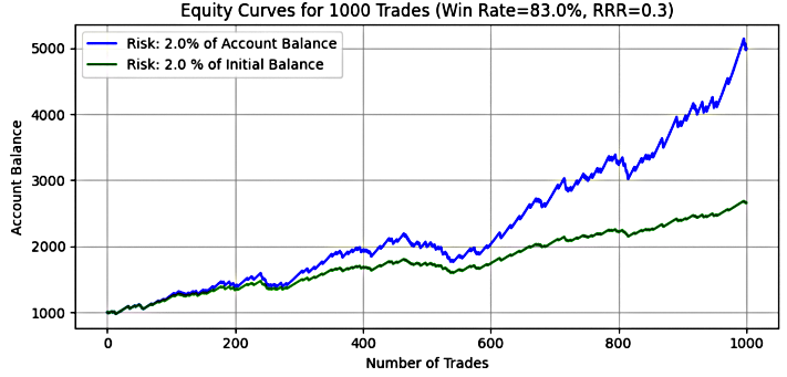
Figure 14 

Table 9: Monte Carlo Simulation results for a system with win-rate=83%, RRR=0.3, 2% risk

Metrics	Dynamic (2% of Current Balance)	Fixed (2% of Initial Balance)
Mean Final Balance	$4,842.45	$2,581.46
Median Final Balance	$4,621.22	$2,580.00
Min Final Balance	$2,052.24	$1,774.00
Max Final Balance	$11,256.45	$3,464.00
Mean Drawdown	$443.14	$144.99
Median Drawdown	$407.10	$136.00
Max Drawdown	$1,214.00	$286.00
Mean Max Drawdown (%)	13.77%	9.42%
Median Max Drawdown (%)	13.13%	8.63%
Max Drawdown (%)	25.67%	21.47%

Key Insight:

At 2% risk, the performance divergence between dynamic and fixed models becomes clearer. Dynamic risk produced a mean final balance of $4,842.45 (almost 5x starting capital), compared to $2,581.46 under fixed risk (2.6x). The median final balances closely matched the means, confirming predictability and consistent performance.

The maximum final balance under dynamic risk hit $11,256.45, indicating that a few strong streaks can produce substantial growth, while fixed risk peaked at $3,464. However, maximum drawdowns also increased, with dynamic risk hitting25.67%, and fixed risk maintaining a lower 21.47%.

This scenario reflects a moderate risk-reward profile where compounding under dynamic risk enhances returns, while fixed risk offers lower volatility with limited upside.

•  5% risk level

Figure 15 

Table 10: Monte Carlo Simulation results for a system with win-rate=83%, RRR=0.3, 5% risk

Metrics	Dynamic (1% of Current Balance)	Fixed (1% of Initial Balance)
Mean Final Balance	$50,642.20	$4,953.64
Median Final Balance	$38,003.88	$4,950.00
Min Final Balance	$4,884.41	$2,935.00
Max Final Balance	$360,637.45	$7,160.00
Mean Drawdown	$9,127.86	$362.48
Median Drawdown	$7,201.27	$340.00
Max Drawdown	$62,063.85	$715.00
Mean Max Drawdown (%)	31.82%	18.15%
Median Max Drawdown (%)	30.97%	16.25%
Max Drawdown (%)	54.29%	49.28%

Key Insight:

At 5% risk, the system's potential explodes under dynamic risk, yielding a mean final balance of over $50,000 (50x initial capital) and a median of $38,003, indicating a strong bias toward profitable outcomes. The maximum final balance was an extraordinary $360,637, confirming the system’s ability to compound small wins into massive returns.

However, this comes at the cost of high volatility—with mean drawdowns exceeding $9,000 and maximum drawdowns hitting over $62,000. The mean drawdown percentage was nearly 32%, and the worst-case scenario reached 54.29%, which could still be tolerable for well-capitalized traders but may challenge psychological resilience.

For fixed risk, the performance was more contained. The mean final balance was$4,953.64 (about 5x capital), with a maximum of $7,160. Drawdowns were significantly lower than dynamic, with median max drawdown around 16%, and maximum drawdown capped at 49.28%.

Recommended Risk Levels for System 5 (83% Win Rate, RRR = 0.3)

For a system with such a high win rate and low RRR, the simulations affirm it is statistically stable and resilient, especially under conservative risk.

• 1% to 2% risk of current balance is optimal for most traders—offering a balance of consistency, growth, and manageable drawdowns.
• Dynamic risk enhances performance through compounding but introduces slightly higher drawdowns.
• Fixed risk produces a more predictable equity curve, suited for traders prioritizing low volatility.

At 5% risk, dynamic risk delivers exceptional upside but demands emotional discipline to endure drawdowns in the 30–50% range. Fixed risk at 5% yields predictable 5x returns with maximum drawdowns under 50%, making it attractive to traders seeking steady results without extreme swings.

For some traders, risking5% of the initial balance may be a preferred approach for this system, given its low mean and median drawdown percentages and a predictable return potential of approximately 5x the initial capital. Although the worst-case drawdown reached 49.28%, it was a statistically rare outcome in the simulations and could be tolerable for traders comfortable with moderate risk exposure.

For others, risking 5% of the current balance (dynamic model) may be more appealing due to its exceptional return potential, with a mean final balance exceeding 50x and a median of 38x the initial equity. Despite the aggressive risk sizing, the system exhibited moderate drawdown behavior, with mean and median drawdowns around 32%, and a maximum drawdown of 54.29%. While this level of volatility is significant, it remains within acceptable limits for experienced traders who are prepared—both emotionally and financially—for a high-compounding, high-variability strategy.

For this system, risking beyond the traditional 2% rule is a viable path to achieving trading objectives, but it requires a robust and reliable trading system to carry you through periods of drawdown and reach your target.

Code Usage

To evaluate alternative outcomes, modify the parameter values in the following section. This allows for flexible testing under varying conditions while maintaining the underlying analytical framework.

# Parameters
win_rate = 0.83
rrr = 0.3
num_trades = 1000
initial_balance = 1000
risk_percent = 0.05  # %

np.random.seed(42)

#The use of a predefined seed (e.g., 42) enables result reproducibility. 
#Users may change this value/deactivate the seeding logic by commenting out the relevant code block.

Conclusion

In this article, we applied Monte Carlo simulation to objectively quantify the impact of consecutive losing streaks and explore how they interact with different win-rate systems and position sizing strategies. The results indicate that trading systems with lower win rates tend to experience longer losing streaks, while higher win-rate systems experience shorter and less frequent streaks.

However, despite the psychological challenges associated with low win-rate systems, those with positive expectancy (i.e., a sufficiently high reward-to-risk ratio) can deliver significantly higher returns when exposed to the same risk levels. This reinforces the point that win rate alone doesn't define profitability—expectancy and risk management are just as important.

Our analysis also revealed that drawdown severity is directly influenced by both the length of losing streaks and the level of risk per trade. Naturally, the higher the risk, the greater the potential drawdown—but also the greater the potential reward, especially for systems with a mathematical edge.

While the traditional 1%-2% risk rule remains a sound foundation, our results suggest that traders with a robust and proven system can justify going beyond the 2% threshold. For example, the 83% win-rate, RRR = 0.3 system demonstrated stable drawdowns even at 5% risk, particularly under the fixed risk model. In fact, if such a system had a slightly better RRR (e.g., 0.5), risking more than 2% could be even more viable—though this should be tested thoroughly using simulation tools.

Overall, our simulations consistently showed that dynamic risk (based on current balance) outperformed fixed risk in terms of long-term returns. However, fixed risk models offered more stable and predictable outcomes in certain cases—such as the 5% risk setting in the 65% win-rate, RRR = 0.9 system.

This raises a broader question: Can we set specific trading targets and reliably achieve them using a well-defined trading system?

We believe this is at the heart of successful trading—turning strategy into targeted results. In the next article, we will explore this concept further and demonstrate how traders can set and pursue realistic profit goals using simulation-backed strategies.