Finding seasonal patterns in the forex market using the CatBoost algorithm

Introduction

Two other articles devoted to seasonal pattern search have already been published (1, 2). I was wondering how machine learning algorithms can cope with the pattern search task. Trading systems in the above-mentioned articles were built on the basis of statistical analysis. The human factor can be eliminated now by simply instructing the model to trade at a certain hour of a certain day of the week. Pattern search can be provided by a separate algorithm.

Time filtering function

The library can be easily extended by adding a filter function.

def time_filter(data, count):
    # filter by hour
    hours=[15]
    if data.index[count].hour not in hours:
        return False

    # filter by day of week
    days = [1]
    if data.index[count].dayofweek not in days:
        return False

    return True

The function checks the conditions specified inside it. Other additional conditions can be implemented (not only time filters). But since the article is devoted to seasonal patterns, I will only use time filters. If all the conditions are met, the function returns True and the appropriate sample is added to the training set. For example, in this particular case, we instruct the model to open trades only at 15:00 on Tuesday. The 'hours' and 'days' lists can include other hours and days. By commenting out all the conditions, you can let the algorithm work without conditions, the way it worked in the previous article. 

The add_labels function now receives this condition as an input. In Python, functions are first-level objects, so you can safely pass them as arguments to other functions.

def add_labels(dataset, min, max, filter=time_filter):
    labels = []
    for i in range(dataset.shape[0]-max):
        rand = random.randint(min, max)
        curr_pr = dataset['close'][i]
        future_pr = dataset['close'][i + rand]
        if filter(dataset, i):
            if future_pr + MARKUP < curr_pr:
                labels.append(1.0)
            elif future_pr - MARKUP > curr_pr:
                labels.append(0.0)
            else:
                labels.append(2.0)
        else:
            labels.append(2.0)
    dataset = dataset.iloc[:len(labels)].copy()
    dataset['labels'] = labels
    dataset = dataset.dropna()
    dataset = dataset.drop(
        dataset[dataset.labels == 2].index)

    return dataset

As soon as the filter is passed to the function, it can be used to mark Buy or Sell trades. The filter receives the original dataset and the index of the current bar. Indexes in the dataset are represented as 'datetime index' containing the time. The filter searches for the hour and day in the dataframe's 'datetime index' by the i-th number and returns False if it finds nothing. If the condition is met, the deal is marked as 1 or 0, otherwise as 2. Finally, all 2s are removed from the training dataset, and thus only examples for specific days and hours determined by the filter are left.

A filter should also be added to the custom tester, to enable trade opening at a specific time (or according to any other condition set by this filter).

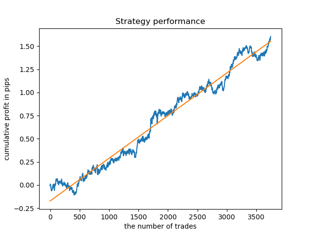
def tester(dataset, markup=0.0, plot=False, filter=time_filter):
    last_deal = int(2)
    last_price = 0.0
    report = [0.0]
    for i in range(dataset.shape[0]):
        pred = dataset['labels'][i]
        ind = dataset.index[i].hour
        if last_deal == 2 and filter(dataset, i):
            last_price = dataset['close'][i]
            last_deal = 0 if pred <= 0.5 else 1
            continue
        if last_deal == 0 and pred > 0.5:
            last_deal = 2
            report.append(report[-1] - markup +
                          (dataset['close'][i] - last_price))
            continue
        if last_deal == 1 and pred < 0.5:
            last_deal = 2
            report.append(report[-1] - markup +
                          (last_price - dataset['close'][i]))

    y = np.array(report).reshape(-1, 1)
    X = np.arange(len(report)).reshape(-1, 1)
    lr = LinearRegression()
    lr.fit(X, y)

    l = lr.coef_
    if l >= 0:
        l = 1
    else:
        l = -1

    if(plot):
        plt.plot(report)
        plt.plot(lr.predict(X))
        plt.title("Strategy performance")
        plt.xlabel("the number of trades")
        plt.ylabel("cumulative profit in pips")
        plt.show()

    return lr.score(X, y) * l

This is implemented as follows. Digit 2 is used when there is no open position: last_deal = 2. There are no open positions before testing start, therefore set 2. Iterate through the entire dataset and check if the filter condition is met. If the condition is met, open a Buy or Sell deal. The filter conditions do not apply to deal closing, as they can be closed at another hour or day of the week. These changes are enough for further correct training and testing. 

Exploratory analysis for each trading hour

It is not very convenient to test the model manually for each individual condition (and for a combination of hours or days). A special function has been written for this purpose, which allows fast obtaining of summary statistics for each condition separately. The function may take some time to complete, but it outputs the time ranges in which the model shows better performance.

def exploratory_analysis():
    h = [x for x in range(24)]
    result = pd.DataFrame()
    for _h in h:
        global hours 
        hours = [_h]
        pr = get_prices(START_DATE, STOP_DATE)
        pr = add_labels(pr, min=15, max=15, filter=time_filter)
        gmm = mixture.GaussianMixture(
            n_components=n_compnents, covariance_type='full', n_init=1).fit(pr[pr.columns[1:]])

        # iterative learning
        res = []
        iterations = 10
        for i in range(iterations):
            res.append(brute_force(10000, gmm))
            print('Iteration: ', i, 'R^2: ', res[-1][0], ' hour= ', _h)
        
        r = pd.DataFrame(np.array(res)[:, 0], np.full(iterations,_h))
        result = result.append(r)

    plt.scatter(result.index, result, c = result.index)
    plt.show()
    return result

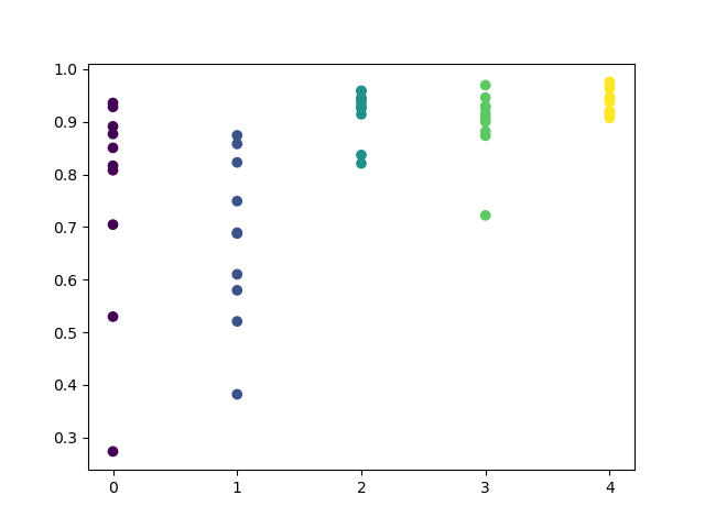
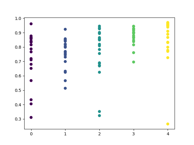
You can set in the function a list of hours to be checked. In my example all 24 hours are set. For the purity of the experiment, I disabled sampling by setting 'min' and 'max' (minimum and maximum horizon of an open position) equal to 15. The 'iterations' variable is responsible for the number of retraining cycles for each hour. A more reliable statistics can be obtained by increasing this parameter. After completing operation, the function will display the following graph:

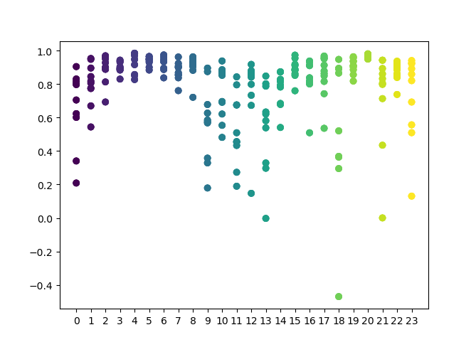
The X-axis features the ordinal numbers of the hours. The Y-axis represents R^2 scores for each iteration (10 iterations were used, which means model retraining for each hour). As you can see, passes for hours 4, 5 and 6 hours are located more closely, which gives more confidence in the quality of the found pattern. The selection principle is simple — the higher the position and density of the points, the better the model. For example, in the interval of 9-15, the graph shows a large dispersion of points, and the average quality of models drops to 0.6. You can further select the desired hours, retrain the model and view its results in the custom tester.

Testing selected models

The exploratory analysis was performed on the GBPUSD currency pair, with the following parameters:

SYMBOL = 'GBPUSD'
MARKUP = 0.00010
TIMEFRAME = mt5.TIMEFRAME_H1
START_DATE = datetime(2017, 1, 1)
TSTART_DATE = datetime(2015, 1, 1)
FULL_DATE = datetime(2015, 1, 1)
STOP_DATE = datetime(2021, 1, 1)

The same parameters will be used for testing. For greater confidence, you can change the FULL_DATE value to view how the model performed in earlier historic data.

We can visually distinguish a cluster of hours 3, 4, 5 and 6. It can be assumed that adjacent hours have similar patterns, so the model can be trained for all this hour.

hours = [3,4,5,6]
# make dataset
pr = get_prices(START_DATE, STOP_DATE)
pr = add_labels(pr, min=15, max=15, filter=time_filter)
tester(pr, MARKUP, plot=True, filter=time_filter)

# perform GMM clasterizatin over dataset
# gmm = mixture.BayesianGaussianMixture(n_components=n_compnents, covariance_type='full').fit(X)
gmm = mixture.GaussianMixture(
    n_components=n_compnents, covariance_type='full', n_init=1).fit(pr[pr.columns[1:]])

# iterative learning
res = []

for i in range(10):
    res.append(brute_force(10000, gmm))
    print('Iteration: ', i, 'R^2: ', res[-1][0])

# test best model
res.sort()
test_model(res[-1])

No additional explanation is needed for the rest code, as it was explained in detail in previous articles. With the only exception, that instead of a simple GMM you can use a commented Bayesian model, although it is only an experimental idea. 

An ideal model after deal sampling would look like this:

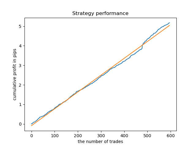
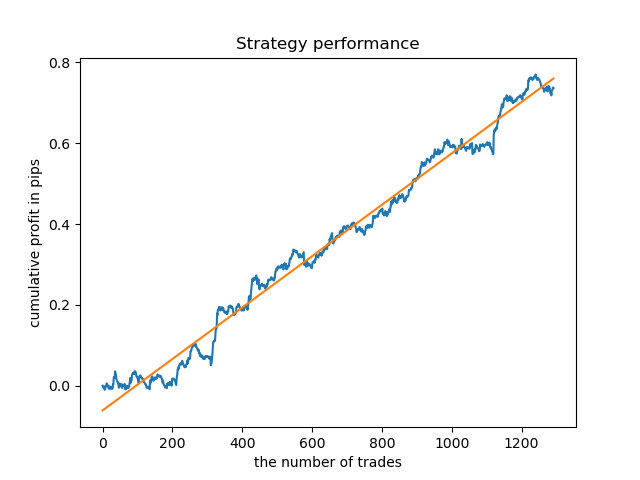
The trained model (including test data) shows the following performance:

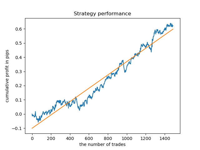
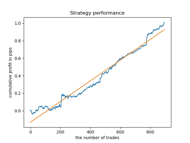
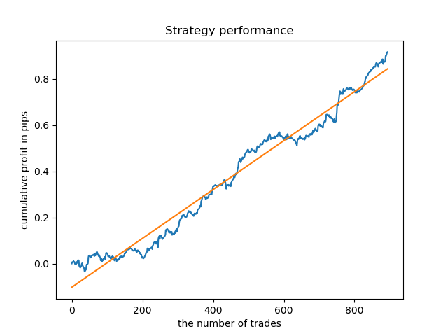
Separate models can be trained for high-density hours. Below are balance graphs for already trained models for hours 5 and 20:

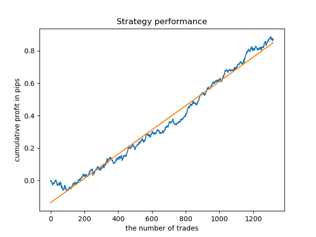
Now, for comparison, you can look at the models trained on hours with larger variance. View hours 9 and 11 for example.

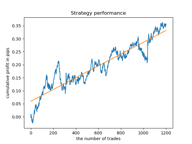
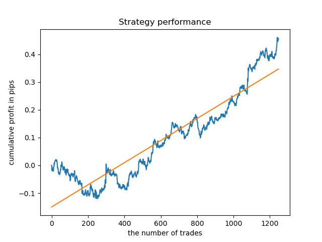
Balance graphs here show more than any comments. Obviously, when training models, special attention should be paid to timing. 

Exploratory analysis for each trading day

The filter can be easily modified for other time intervals, such as for example days of the week. You simply need to replace hour with a day of the week.

def time_filter(data, count):
    # filter by day of week
    global hours
    if data.index[count].dayofweek not in hours:
        return False
    return True

In this case, the iteration should be performed in the range between 0 and 5 (excluding the 5th ordinal number, which is Saturday).

def exploratory_analysis():
    h = [x for x in range(5)]

Now, perform exploratory analysis for the GBPUSD currency pair. The frequency of deals, or their horizon, is the same (15 bars).

pr = add_labels(pr, min=15, max=15, filter=time_filter)

The training process is displayed in the console, where you can instantly view the R^2 scores for the current period. The 'hour' variable now contains not the hour number, but the ordinal number of the day of the week.

Iteration:  0 R^2:  0.5297625368835237  hour=  0
Iteration:  1 R^2:  0.8166096906047893  hour=  0
Iteration:  2 R^2:  0.9357674260125702  hour=  0
Iteration:  3 R^2:  0.8913802241811986  hour=  0
Iteration:  4 R^2:  0.8079720208707672  hour=  0
Iteration:  5 R^2:  0.8505663844866759  hour=  0
Iteration:  6 R^2:  0.2736870273207084  hour=  0
Iteration:  7 R^2:  0.9282442121644887  hour=  0
Iteration:  8 R^2:  0.8769775718602929  hour=  0
Iteration:  9 R^2:  0.7046666925774866  hour=  0
Iteration:  0 R^2:  0.7492883761480897  hour=  1
Iteration:  1 R^2:  0.6101962958733655  hour=  1
Iteration:  2 R^2:  0.6877652983219245  hour=  1
Iteration:  3 R^2:  0.8579669286548137  hour=  1
Iteration:  4 R^2:  0.3822441930760343  hour=  1
Iteration:  5 R^2:  0.5207801806491617  hour=  1
Iteration:  6 R^2:  0.6893157850263495  hour=  1
Iteration:  7 R^2:  0.5799059801202937  hour=  1
Iteration:  8 R^2:  0.8228326786957887  hour=  1
Iteration:  9 R^2:  0.8742262956151615  hour=  1
Iteration:  0 R^2:  0.9257707800422799  hour=  2
Iteration:  1 R^2:  0.9413981795880517  hour=  2
Iteration:  2 R^2:  0.9354221623113591  hour=  2
Iteration:  3 R^2:  0.8370429185837882  hour=  2
Iteration:  4 R^2:  0.9142875737195697  hour=  2
Iteration:  5 R^2:  0.9586871067966855  hour=  2
Iteration:  6 R^2:  0.8209392060391961  hour=  2
Iteration:  7 R^2:  0.9457287035542066  hour=  2
Iteration:  8 R^2:  0.9587372191281025  hour=  2
Iteration:  9 R^2:  0.9269140213952402  hour=  2
Iteration:  0 R^2:  0.9001009579436263  hour=  3
Iteration:  1 R^2:  0.8735623527502183  hour=  3
Iteration:  2 R^2:  0.9460714774572146  hour=  3
Iteration:  3 R^2:  0.7221720163838841  hour=  3
Iteration:  4 R^2:  0.9063579778744433  hour=  3
Iteration:  5 R^2:  0.9695391076372475  hour=  3
Iteration:  6 R^2:  0.9297881558889788  hour=  3
Iteration:  7 R^2:  0.9271590681844957  hour=  3
Iteration:  8 R^2:  0.8817985496711311  hour=  3
Iteration:  9 R^2:  0.915205007218742   hour=  3
Iteration:  0 R^2:  0.9378516360378022  hour=  4
Iteration:  1 R^2:  0.9210968481902528  hour=  4
Iteration:  2 R^2:  0.9072205941748894  hour=  4
Iteration:  3 R^2:  0.9408826184927528  hour=  4
Iteration:  4 R^2:  0.9671981453714584  hour=  4
Iteration:  5 R^2:  0.9625144032389237  hour=  4
Iteration:  6 R^2:  0.9759244293257822  hour=  4
Iteration:  7 R^2:  0.9461473783201281  hour=  4
Iteration:  8 R^2:  0.9190627222826241  hour=  4
Iteration:  9 R^2:  0.9130350931314233  hour=  4

Please note that all models were trained using the data since the beginning of 2017, while the R^2 scores also include the test period (additional data starting from 2015). Consistency of high estimates for each day provides even more confidence. Let us view the final result.

Exploratory analysis has shown that Wednesday and Friday are the most favorable days for trading, especially Friday. The worst day for trading is Tuesday, as it has a large variance of errors and a low average value. Let us train the model to trade only on Fridays and see the result.

Similarly, we can obtain a model trading on Tuesdays.

A fixed lifetime of deals is not always suitable, so let us try to expand the search window and increase the number of exploratory analysis iterations to 20.

pr = add_labels(pr, min=5, max=25, filter=time_filter)
        gmm = mixture.GaussianMixture(
            n_components=n_compnents, covariance_type='full', n_init=1).fit(pr[pr.columns[1:]])

        # iterative learning
        res = []
        iterations = 20

The range of values has become larger, while the best days for trading are Thursday and Friday.

Let us now train a control model for Thursday to see the result. This is how the learning cycle looks like (for those who have not read the previous articles).

hours = [3]
# make dataset
pr = get_prices(START_DATE, STOP_DATE)
pr = add_labels(pr, min=5, max=25, filter=time_filter)
tester(pr, MARKUP, plot=True, filter=time_filter)

# perform GMM clasterizatin over dataset
# gmm = mixture.BayesianGaussianMixture(n_components=n_compnents, covariance_type='full').fit(X)
gmm = mixture.GaussianMixture(
    n_components=n_compnents, covariance_type='full', n_init=1).fit(pr[pr.columns[1:]])


# iterative learning
res = []
for i in range(10):
    res.append(brute_force(10000, gmm))
    print('Iteration: ', i, 'R^2: ', res[-1][0])

# test best model
res.sort()
test_model(res[-1])

The result is slightly worse than with a fixed lifetime of deals. 

Obviously, the frequency (horizon) parameter in specific periods is important. Next, let us iterate over these values and check how they affect the result.

Assessment of the influence of the deal lifetime on the model quality

Similar to the exploratory analysis function for a selected criterion (filter), we can create an auxiliary function which will evaluate the model performance depending on the deal lifetime. Suppose we can set a fixed deal lifetime in the interval from 1 to 50 bars (or any other period), then the function will look as follows.

def deals_frequency_analyzer():
    freq = [x for x in range(1, 50)]
    result = pd.DataFrame()
    for _h in freq:
        pr = get_prices(START_DATE, STOP_DATE)
        pr = add_labels(pr, min=_h, max=_h, filter=time_filter)
        gmm = mixture.GaussianMixture(
            n_components=n_compnents, covariance_type='full', n_init=1).fit(pr[pr.columns[1:]])

        # iterative learning
        res = []
        iterations = 5
        for i in range(iterations):
            res.append(brute_force(10000, gmm))
            print('Iteration: ', i, 'R^2: ', res[-1][0], ' deal lifetime = ', _h)
        
        r = pd.DataFrame(np.array(res)[:, 0], np.full(iterations,_h))
        result = result.append(r)

    plt.scatter(result.index, result, c = result.index)
    plt.xticks(np.arange(0, len(freq)+1, 1))
    plt.title("Performance by deals lifetime")
    plt.xlabel("deals frequency")
    plt.ylabel("R^2 estimation")
    plt.show()
    return result

The 'freq' list contains the values of deal lifetime to iterate over. I performed this iteration for the 5th hour of the GBPUSD pair. Here is the result.

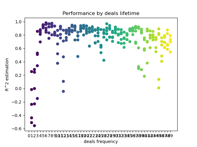
The X axis shows the deal frequency, or rather their lifetime in bars. The Y axis represents the R^2 score for each of the passes. As you can see, too short trades of 0-5 bars have a negative effect on the model performance, while the lifetime of 15-23 is optimal. Longer deals (over 30 bars) worsen the result. There is a small cluster with the deal lifetime of 6-9 bars, which have the highest scores. Let us try to train models with these lifetime values and compare the results with other clusters.

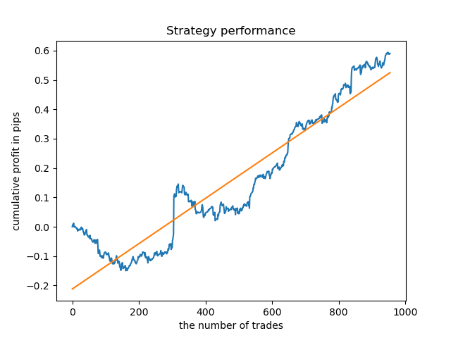
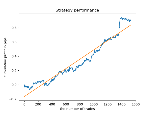
I have selected the lifetime of 8 bars, for which the model was tested since 2013. But the balance curve is not as even as I would like it to be.

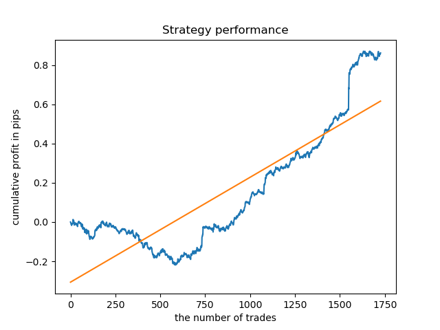
For the lifetime of the cluster with the highest density, the graph looks very good since 2015, however, the model performs poorly at an earlier historic interval.

Finally, I have selected a range of the best clusters 15-23 and retrained the model several times (since the sampling of the trade lifetime is random). 

pr = add_labels(pr, min=15, max=23, filter=time_filter)

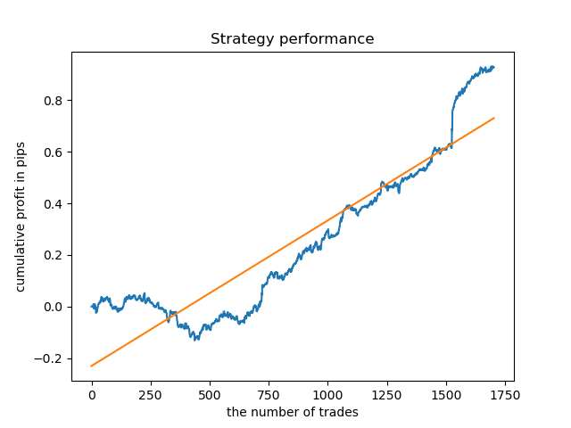
A model based on such patterns does not show survivability on data before 2015. Probably, there were some cardinal changes in the market structure. A separate big study is needed to analyze this situation. After the model has been selected and its stability has been proven over a certain time interval, training can be performed over this entire interval, including a test sample. This model can then be sent to production.

Testing on a longer history

What if we check the model on a longer history? The model was trained on data since 2000 and tested using data since 1990. Patterns are poorly captured on such a long historic period, which can be seen from the balance curve, but the result is still positive.

Conclusion

The article provides a description of a powerful tool for finding seasonal patterns and creating trading systems. You can analyze it for different instruments (other than FOREX), different timeframes and with different filters (not only time filters). The range of application of this approach is very wide. To fully reveal its capabilities, we would need multiple tests with different filters. After conducting the analysis, you can build a trading robot using the model export function described in the previous articles.