Metamodels in machine learning and trading: Original timing of trading orders

Introduction

A distinctive feature of some trading systems is selective trading, which means they are not constantly in the market. For the most part, this is due to the presence of patterns at certain points in time, while at other times the patterns are absent or undefined.

In the previous articles, I have described in detail the various ways, in which machine learning models can be applied to time series classification tasks. All these models were trained "as is" on the training set and compiled into bots after training. The process of labeling the training dataset and choosing the best model was automated as much as possible, which eliminated the human factor almost completely. With all the elegance of the proposed approaches, these models have two drawbacks that would be difficult to fix without introducing additional functionality.

I set out to expand the approach to the cases where the model can:

1. adapt to the training dataset choosing the best examples for training
2. sort out the parts of the time series that are difficult to classify and skip them during training and trading

This generalization made me partially reconsider the approach to training. It turned out that the use of only one classifier does not meet the new requirements. It cannot correct itself while training. Therefore, I decided to change the functionality for the mentioned cases.

Theoretical aspects of the new approach

First, I need to make a small remark. Since the researcher deals with uncertainty while developing trading systems (including the ones applying machine learning), it is impossible to strictly formalize the object of search. It can be defined as some more or less stable dependencies in a multidimensional space that are difficult to interpret in human and even mathematical languages. It is difficult to conduct a detailed analysis of what we get from highly parameterized self-training systems. Such algorithms require a certain degree of trust from a trader based on the results of backtests, but they do not clarify the very essence and even the nature of the pattern found.

I want to write an algorithm that will be able to analyze and correct its own errors iteratively improving its results. To do this, I propose to take a bunch of two classifiers and train them sequentially as suggested in the following diagram. The detailed description of the idea is provided below.

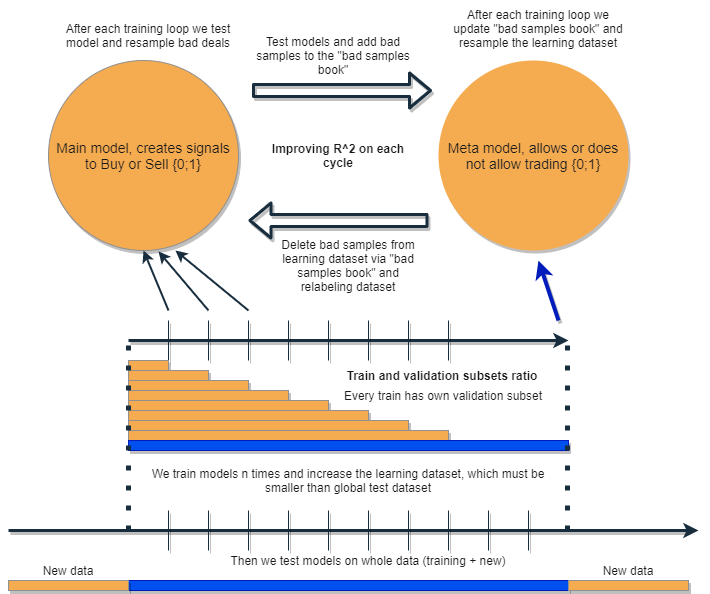
Each of the classifiers is trained on its own dataset, which has its own size. The blue horizontal line represents the conditional history depth for the metamodel, and the orange ones stand for the base model. In other words, the depth of history for a metamodel is always greater than for the base one and is equal to the estimated (test) time interval, on which the combination of these models will be tested.

The bunch of models is retrained several times, while the training dataset for the base model can gradually increase (increasing the length of the orange columns at each new iteration), but its length should not exceed the length of the blue one. After each iteration, all examples that were classified by the metamodel as false (or zero) are removed from the training sample of the base model. The metamodel, in turn, continues to train on all examples.

The intuition behind this approach is that losing trades are Class I classification errors for the underlying model according to the terminology of the confusion matrix. In other words, these are the cases it classifies as false positives. The metamodel filters out such cases and gives a score of 1 for true positives and 0 for everything else. By sorting the dataset for training the base model via the metamodel, we increase its Precision, i.e. the number of correct buy and sell triggers. At the same time, the metamodel increases its Recall (completeness) classifying as many different outcomes as possible. 

The higher the accuracy, the more accurate the model. But in real situations, an improvement in one indicator leads to a deterioration in another within the same classifier, so using the bunch of two classifiers looks like an interesting idea leading to an improvement in both indicators. 

The idea is that the two models are trained on the same attributes and therefore have additional interaction. Due to the increased selection for the metamodel (blue horizontal column compared to orange ones), it leaves good trading situations as if sorting out the errors of the base model on new data for it. By interacting with each other, the models iteratively improve due to relabeling, and the R^2 score on the validation set is constantly increasing. But the metamodel can be trained on its own attributes as a filter for the base model. Such connection does not quite fit into the framework of the proposed approach, therefore it is not considered here.

The base model should work well due to the constant "maintenance" of the metamodel, but the metamodel itself can also be wrong. For example, the first iteration revealed cases that were not suitable for trading. In the second iteration, after retraining the base model and adjusting the examples for the metamodel, bad examples may differ from those in the previous iteration. Because of this, the metamodel may tend to constantly relabel examples that will differ from iteration to iteration. This behavior may never reach the balance. To fix this shortcoming, let's create the "bad samples book" table, which will be updated with examples from all previous iterations. More specifically, it will store feature values at times marked as bad for trading at all previous training iterations. This will allow updating the dataset of the metamodel before each retraining in such a way that all unsuccessful moments from previous iterations will also be marked as bad (zeros).

The "bad samples book" also has its disadvantage, since too many iterations will add too many zeros (bad trades). The number of examples will decrease significantly for each new training iteration. Therefore, it is necessary to find a balance between the number of iterations and the number of examples added to the bad samples book. The situation can be partially solved by averaging the number of bad examples depending on the time of their occurrence and sorting only the most common ones. The metamodel dataset will not degenerate in this case (the balance between zeros and ones will remain). It would be good to use oversampling if the classes turn out to be highly unbalanced.

After several iterations, this bunch of models will show excellent results on training and validation data. Moreover, the result will improve from iteration to iteration. After training, the bunch of models should be tested on completely new data, which can be located both earlier and later in time than the training subsample. There is no theory that makes it possible to unequivocally state which part of history should be chosen for tests on non-stationary financial time series. Nevertheless, I expect the improvement in the performance of the proposed approach on new data, while real practice will show the rest.

So, we train a single model, correct its errors on new data with another model and repeat this process several times. Why should this increase the robustness of the classifiers on new data? There is no single answer to this question. There is an assumption that we are dealing with some kind of a pattern. If it exists, it will be found, and situations without a pattern will be sorted out. If the pattern is stable, then the model will work on new data.

In theory, this approach should kill two birds with one stone:

• provide a high expectation of profitable trades
• do auto "timing" of the trading system, trading only at certain highly effective points in time

Since we are talking about the timing of the trading system, we should touch on one more interesting point. Now the dependence on the choice of attributes (features) for the model is reduced.

The basic approach and supervised markup imply a scrupulous selection of predictors and targets. In fact, this is the main issue of this approach. Data preparation and analysis always have top priority, while the quality of models directly depends on the professionalism of an analyst in a particular area (in our case, it is FOREX).

The proposed approach should automatically find interrelated timing, predictor and label events, and exploit the automatically found patterns. The choice of predictors and the labeling of deals occur automatically. It is still necessary to comply with a number of conditions: for example, the attributes should be stationary and have at least an indirect relation to the financial instrument. But in a situation where the true patterns are unknown to us and there is nowhere to get information from, this approach looks justified.

Of course, if we work with "garbage" attributes having no causal relationship with deals, the algorithm will work randomly. However, this is already a question of the presence/absence of cause-and-effect relationships as such. This article deliberately does not consider the construction of features other than increments (the difference between a moving average and a price), since this is a separate huge topic that may be considered in other articles. It is assumed that the analytical approach to the selection of informative features should significantly increase the stability of the algorithm on new data.

Practical implementation of the proposed approach

As usual, everything looks wonderful in theory. Now let's check what effect can actually be obtained from a bunch of two classifiers. To do this, we need to rewrite the code again.

The function of deals auto markup

I have made some changes. Now it is possible to relabel the labels for the base models based on the metamodel labels:

def labelling_relabeling(dataset, min=15, max=15, relabeling=False) -> pd.DataFrame:
    labels = []
    for i in range(dataset.shape[0]-max):
        rand = random.randint(min, max)
        curr_pr = dataset['close'][i]
        future_pr = dataset['close'][i + rand]

        if relabeling:
            m_labels  = dataset['meta_labels'][i:rand+1].values
        
        if relabeling and 0.0 in m_labels:
            labels.append(2.0)
        else:
            if future_pr + MARKUP < curr_pr:
                labels.append(1.0)
            elif future_pr - MARKUP > curr_pr:
                labels.append(0.0)
            else:
                labels.append(2.0)
        
    dataset = dataset.iloc[:len(labels)].copy()
    dataset['labels'] = labels
    dataset = dataset.dropna()
    dataset = dataset.drop(
        dataset[dataset.labels == 2].index)

    return dataset

The highlighted code checks for the presence of the relabel flag. If it is True and the current trade horizon metatags contain zeros, then the metamodel rejects trading on this section. Accordingly, such deals are marked as 2.0 and removed from the dataset. Thus, we are able to carry out iterative removal of unnecessary samples from the training sample for the base model reducing the error of its training.

Custom tester function

Now there is an extended functionality that allows us to test two models at once (base and meta). In addition, the custom tester is now able to relabel the labels for the metamodel in order to improve it at the next iteration.

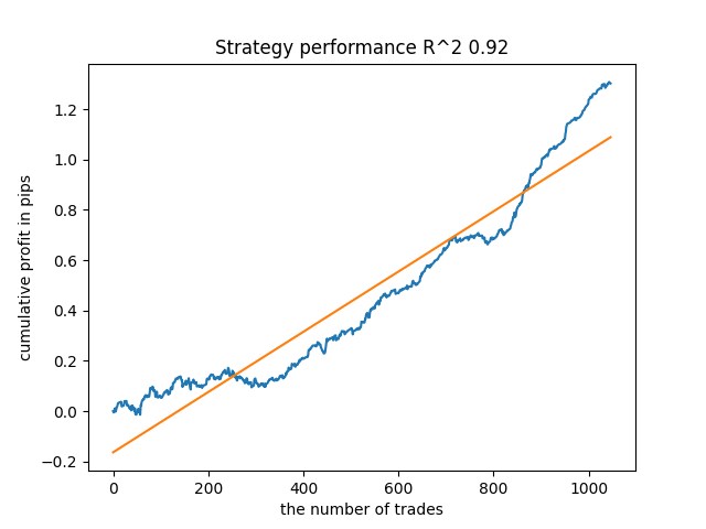
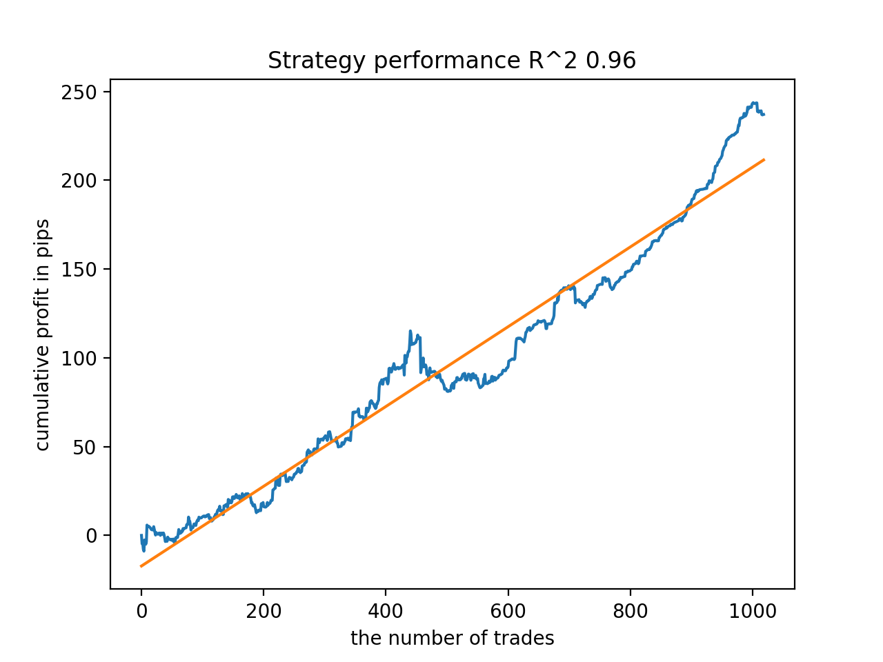
def tester(dataset: pd.DataFrame, markup=0.0, use_meta=False, plot=False):
    last_deal = int(2)
    last_price = 0.0
    report = [0.0]
    meta_labels = dataset['labels'].copy()

    for i in range(dataset.shape[0]):
        pred = dataset['labels'][i]
        meta_labels[i] = np.nan
        if use_meta:
            pred_meta = dataset['meta_labels'][i] # 1 = allow trades

        if last_deal == 2 and ((use_meta and pred_meta==1) or not use_meta):
            last_price = dataset['close'][i]
            last_deal = 0 if pred <= 0.5 else 1
            continue

        if last_deal == 0 and pred > 0.5 and ((use_meta and pred_meta==1) or not use_meta):
            last_deal = 2
            report.append(report[-1] - markup +
                          (dataset['close'][i] - last_price))
            if report[-1] > report[-2]:
                meta_labels[i] = 1
            else:
                meta_labels[i] = 0
            continue

        if last_deal == 1 and pred < 0.5 and ((use_meta and pred_meta==1) or not use_meta):
            last_deal = 2
            report.append(report[-1] - markup +
                          (last_price - dataset['close'][i]))
            if report[-1] > report[-2]:
                meta_labels[i] = 1
            else:
                meta_labels[i] = 0

    y = np.array(report).reshape(-1, 1)
    X = np.arange(len(report)).reshape(-1, 1)
    lr = LinearRegression()
    lr.fit(X, y)

    l = lr.coef_
    if l >= 0:
        l = 1
    else:
        l = -1

    if(plot):
        plt.plot(report)
        plt.plot(lr.predict(X))
        plt.title("Strategy performance R^2 " + str(format(lr.score(X, y) * l,".2f")))
        plt.xlabel("the number of trades")
        plt.ylabel("cumulative profit in pips")
        plt.show()

    return lr.score(X, y) * l, meta_labels.fillna(method='backfill')

The tester works as follows.

If the flag for considering the metamodel during the test is set, the condition for the presence of its signal (one) is checked. If the signal exists, then the base model is allowed to open and close deals, otherwise it does not trade. The light green marker highlights adding new labels for the metamodel depending on the result of a closed deal. If the result is positive, then one is added. Otherwise, the deal is marked as 0 (unsuccessful).

Brute force function 

The biggest changes were made here. I will mark them in the listing with different colors and describe them for better understanding.

def brute_force(dataset, bad_samples_fraction=0.5):
    # features for model\meta models. We learn main model only on filtered labels 
    X = dataset[dataset['meta_labels']==1]
    X = dataset[dataset.columns[:-2]]
    X = X[X.index >= START_DATE]
    X = X[X.index <= STOP_DATE]

    X_meta = dataset[dataset.columns[:-2]]
    X_meta = X_meta[X_meta.index >= TSTART_DATE]
    X_meta = X_meta[X_meta.index <= STOP_DATE]

    # labels for model\meta models
    y = dataset[dataset['meta_labels']==1]
    y = dataset[dataset.columns[-2]]
    y = y[y.index >= START_DATE]
    y = y[y.index <= STOP_DATE]

    y_meta = dataset[dataset.columns[-1]]
    y_meta = y_meta[y_meta.index >= TSTART_DATE]
    y_meta = y_meta[y_meta.index <= STOP_DATE]

    # train\test split
    train_X, test_X, train_y, test_y = train_test_split(
        X, y, train_size=0.5, test_size=0.5, shuffle=True,)

    # learn main model with train and validation subsets
    model = CatBoostClassifier(iterations=1000,
                               depth=6,
                               learning_rate=0.1,
                               custom_loss=['Accuracy'],
                               eval_metric='Accuracy',
                               verbose=False,
                               use_best_model=True,
                               task_type='CPU',
                               random_seed=13)
    model.fit(train_X, train_y, eval_set=(test_X, test_y),
              early_stopping_rounds=50, plot=False)

    # train\test split
    train_X, test_X, train_y, test_y = train_test_split(
        X_meta, y_meta, train_size=0.5, test_size=0.5, shuffle=True)

    # learn meta model with train and validation subsets
    meta_model = CatBoostClassifier(iterations=1000,
                                    depth=6,
                                    learning_rate=0.1,
                                    custom_loss=['Accuracy'],
                                    eval_metric='Accuracy',
                                    verbose=False,
                                    use_best_model=True,
                                    task_type='CPU',
                                    random_seed=13)
    meta_model.fit(train_X, train_y, eval_set=(test_X, test_y),
              early_stopping_rounds=50, plot=False)

    # predict on new data (validation plus learning)
    pr_tst = get_prices()
    X = pr_tst[pr_tst.columns[1:]]
    X.columns = [''] * len(X.columns)
    X_meta = X.copy()

    # predict the learned models (base and meta)
    p = model.predict_proba(X)
    p_meta = meta_model.predict_proba(X_meta)

    p2 = [x[0] < 0.5 for x in p]
    p2_meta = [x[0] < 0.5 for x in p_meta]
    pr2 = pr_tst.iloc[:len(p2)].copy()
    pr2['labels'] = p2
    pr2['meta_labels'] = p2_meta
    pr2['labels'] = pr2['labels'].astype(float)
    pr2['meta_labels'] = pr2['meta_labels'].astype(float)
    full_pr = pr2.copy()
    pr2 = pr2[pr2.index >= TSTART_DATE]
    pr2 = pr2[pr2.index <= STOP_DATE]

    # add bad samples of this iteratin (bad meta labels)
    global BAD_SAMPLES_BOOK
    BAD_SAMPLES_BOOK = BAD_SAMPLES_BOOK.append(pr2[pr2['meta_labels']==0.0].index)
    
    # test mdels and resample meta labels
    R2, meta_labels = tester(pr2, MARKUP, use_meta=True, plot=False)
    pr2['meta_labels'] = meta_labels

    # resample labels based on meta labels
    pr2 = labelling_relabeling(pr2, relabeling=True)
    pr2['labels'] = pr2['labels'].astype(float)
    pr2['meta_labels'] = pr2['meta_labels'].astype(float)

    # mark bad labels from bad_samples_book
    if BAD_SAMPLES_BOOK.value_counts().max() > 1:
        to_mark = BAD_SAMPLES_BOOK.value_counts()
        mean = to_mark.mean()
        marked_idx = to_mark[to_mark > mean*bad_samples_fraction].index
        pr2.loc[pr2.index.isin(marked_idx), 'meta_labels'] = 0.0
    else:
        pr2.loc[pr2.index.isin(BAD_SAMPLES_BOOK), 'meta_labels'] = 0.0

    R2, _ = tester(full_pr, MARKUP, use_meta=True, plot=False)

    return [R2, model, meta_model, pr2]

BAD_SAMPLES_BOOK and the rest of the code highlighted with the appropriate marker is responsible for implementing the bad samples book. At each new iteration of retraining the two models, it is replenished with new examples of unsuccessful deals opened by the previous models after they were trained. The verification is done using the tester.

The last highlighted block can be flexibly configured depending on which part of the failed examples should be marked as 0 at the next retraining. By default, the average of all duplicates for each date contained in the workbook is calculated.

marked_idx = to_mark[to_mark > mean*bad_samples_fraction].index

This is done so that not all bad dates can be removed, but only those, during which the model made the most mistakes while passing all training iterations. The larger the bad_samples_fraction parameter value, the fewer bad dates will be removed, and vice versa.

The blue color denotes that a shortened part of the dataset starting from START_DATE is used for the base model. Earlier data does not participate in its training. However, it participates in the training of the metamodel. Also, this color shows that two different models are being trained - Base and Meta.

The pink color highlights the part where predictions of both models are extracted. A new dataset is formed with the help of these predictions. The dataset is pushed further through the code. The bad metamodel labels are added to the bad samples book from it as well. 

After that, both models are tested in the custom tester, which additionally relabels (adjusts) the metamodel labels for the next training iteration. Further relabeling is carried out for the base model on the corrected dataset.

At the final stage, the dataset is additionally adjusted using the bad samples book and returned by the function for the next training iteration.

Despite the abundance of Python code, it works quickly due to the absence of nested loops and performed optimization. Training CatBoost classifiers takes most of the time. The training time increases with the increase in the number of attributes and the dataset length.

Iterative retraining of models

These were the main details of the new approach. Now it is time to move on to the model training cycle. Let's have a look at everything that happens at each stage.

# make dataset
pr = get_prices()
pr = labelling_relabeling(pr, relabeling=False)
a, b = tester(pr, MARKUP, use_meta=False, plot=False)
pr['meta_labels'] = b
pr = pr.dropna()
pr = labelling_relabeling(pr, relabeling=True)


# iterative learning
res = []
BAD_SAMPLES_BOOK = pd.DatetimeIndex([])
for i in range(25):
    res.append(brute_force(pr[pr.columns[1:]], bad_samples_fraction=0.7))

    print('Iteration: {}, R^2: {}'.format(i, res[-1][0]))
    pr = res[-1][3] 

The first two strings simply create the training dataset, just like in the examples from the previous articles.

>>> pr = get_prices(START_DATE, STOP_DATE)
>>> pr = labelling_relabeling(pr, relabeling=False)
>>> pr
                       close         0         1         2         3         4         5         6  labels       
time
2020-05-06 20:00:00  1.08086  0.000258 -0.000572 -0.001667 -0.002396 -0.004554 -0.007759 -0.009549     1.0       
2020-05-06 21:00:00  1.08032 -0.000106 -0.000903 -0.002042 -0.002664 -0.004900 -0.008039 -0.009938     1.0       
2020-05-06 22:00:00  1.07934 -0.001020 -0.001568 -0.002788 -0.003494 -0.005663 -0.008761 -0.010778     1.0       
2020-05-06 23:00:00  1.07929 -0.000814 -0.001319 -0.002624 -0.003380 -0.005485 -0.008559 -0.010684     1.0       
2020-05-07 00:00:00  1.07968 -0.000218 -0.000689 -0.002065 -0.002873 -0.004894 -0.007929 -0.010144     1.0       
...                      ...       ...       ...       ...       ...       ...       ...       ...     ...       
2021-04-13 23:00:00  1.19474  0.000154  0.002590  0.003375  0.003498  0.004095  0.004273  0.004888     0.0       
2021-04-14 00:00:00  1.19492  0.000108  0.002337  0.003398  0.003565  0.004183  0.004410  0.005001     0.0       
2021-04-14 01:00:00  1.19491 -0.000038  0.002023  0.003238  0.003433  0.004076  0.004353  0.004908     0.0       
2021-04-14 02:00:00  1.19537  0.000278  0.002129  0.003534  0.003780  0.004422  0.004758  0.005286     0.0       
2021-04-14 03:00:00  1.19543  0.000356  0.001783  0.003423  0.003700  0.004370  0.004765  0.005259     0.0       

[5670 rows x 9 columns]

Now we need to add labels for the metamodel. As you might remember, the tester() function returns the R^2 score and a frame with labeled deals. Therefore, we run the tester and add the resulting frame to the original data.

>>> a, b = tester(pr, MARKUP, use_meta=False, plot=False)
>>> pr['meta_labels'] = b
>>> pr = pr.dropna()
>>> pr
                       close         0         1         2  ...         5         6  labels  meta_labels
time                                                        ...
2020-05-06 20:00:00  1.08086  0.000258 -0.000572 -0.001667  ... -0.007759 -0.009549     1.0          1.0
2020-05-06 21:00:00  1.08032 -0.000106 -0.000903 -0.002042  ... -0.008039 -0.009938     1.0          1.0
2020-05-06 22:00:00  1.07934 -0.001020 -0.001568 -0.002788  ... -0.008761 -0.010778     1.0          1.0
2020-05-06 23:00:00  1.07929 -0.000814 -0.001319 -0.002624  ... -0.008559 -0.010684     1.0          1.0
2020-05-07 00:00:00  1.07968 -0.000218 -0.000689 -0.002065  ... -0.007929 -0.010144     1.0          1.0
...                      ...       ...       ...       ...  ...       ...       ...     ...          ...
2021-04-13 18:00:00  1.19385  0.001442  0.003437  0.003198  ...  0.003637  0.004279     0.0          1.0
2021-04-13 19:00:00  1.19379  0.000546  0.003121  0.003015  ...  0.003522  0.004166     0.0          1.0
2021-04-13 20:00:00  1.19423  0.000622  0.003269  0.003349  ...  0.003904  0.004555     0.0          1.0
2021-04-13 21:00:00  1.19465  0.000820  0.003315  0.003640  ...  0.004267  0.004929     0.0          1.0
2021-04-13 22:00:00  1.19552  0.001112  0.003733  0.004311  ...  0.005092  0.005733     1.0          1.0

[5665 rows x 10 columns]

The data is now ready for training. We can make an additional relabeling of the main labels ('labels') according to the second labels ('meta_labels'). In other words, we can remove all deals that turned out to be unprofitable from the dataset.

pr = labelling_relabeling(pr, relabeling=True)

The data is ready, now let's look at the training cycle of both models.

# iterative learning
res = []
BAD_SAMPLES_BOOK = pd.DatetimeIndex([])
for i in range(25):
    res.append(brute_force(pr[pr.columns[1:]], bad_samples_fraction=0.7))

    print('Iteration: {}, R^2: {}'.format(i, res[-1][0]))
    pr = res[-1][3] 

First, we need to reset the bad deals book if there is something left in it after the previous training. Next, the required number of iterations is set in the loop. At each iteration, the nested lists with saved models (and everything else that the brute_force() function returns) are written to the res[] list. For example, we can additionally print the main metrics of the models at each iteration.

The pr variable contains the converted and returned dataset, which will be used for training at the next iteration. 

It is possible to increase the training period of the basic model as suggested in the theoretical part. To achieve this, the start date of training is changed by the specified number of days. At the same time, its size should not exceed the size of the TSTART_DATE interval the metamodel is trained on.

After launching the training, you can see something similar to the following picture:

Iteration: 0, R^2: 0.30121038659012245
Iteration: 1, R^2: 0.7400055934041012
Iteration: 2, R^2: 0.6221261327516192
Iteration: 3, R^2: 0.8892813889403367
Iteration: 4, R^2: 0.787251984980149
Iteration: 5, R^2: 0.794241109825588
Iteration: 6, R^2: 0.9167876214355855
Iteration: 7, R^2: 0.903399695678254
Iteration: 8, R^2: 0.8273236332747745
Iteration: 9, R^2: 0.8646088124681762
Iteration: 10, R^2: 0.8614746864767437
Iteration: 11, R^2: 0.7900599001415054
Iteration: 12, R^2: 0.8837049280116869
Iteration: 13, R^2: 0.784793801426211
Iteration: 14, R^2: 0.941340102099874
Iteration: 15, R^2: 0.8715065229034792
Iteration: 16, R^2: 0.8104990158946458
Iteration: 17, R^2: 0.8542444489379808
Iteration: 18, R^2: 0.8307365677342298
Iteration: 19, R^2: 0.9092509787525882

The first run is usually not very good. Then the model tries to improve itself with each new pass. The models are then sorted in ascending R^2 order and can be tested against new data. We may first look at the evolution of models rather than using sorting right away. A characteristic sign of the evolution is a decrease in the number of deals when testing models.

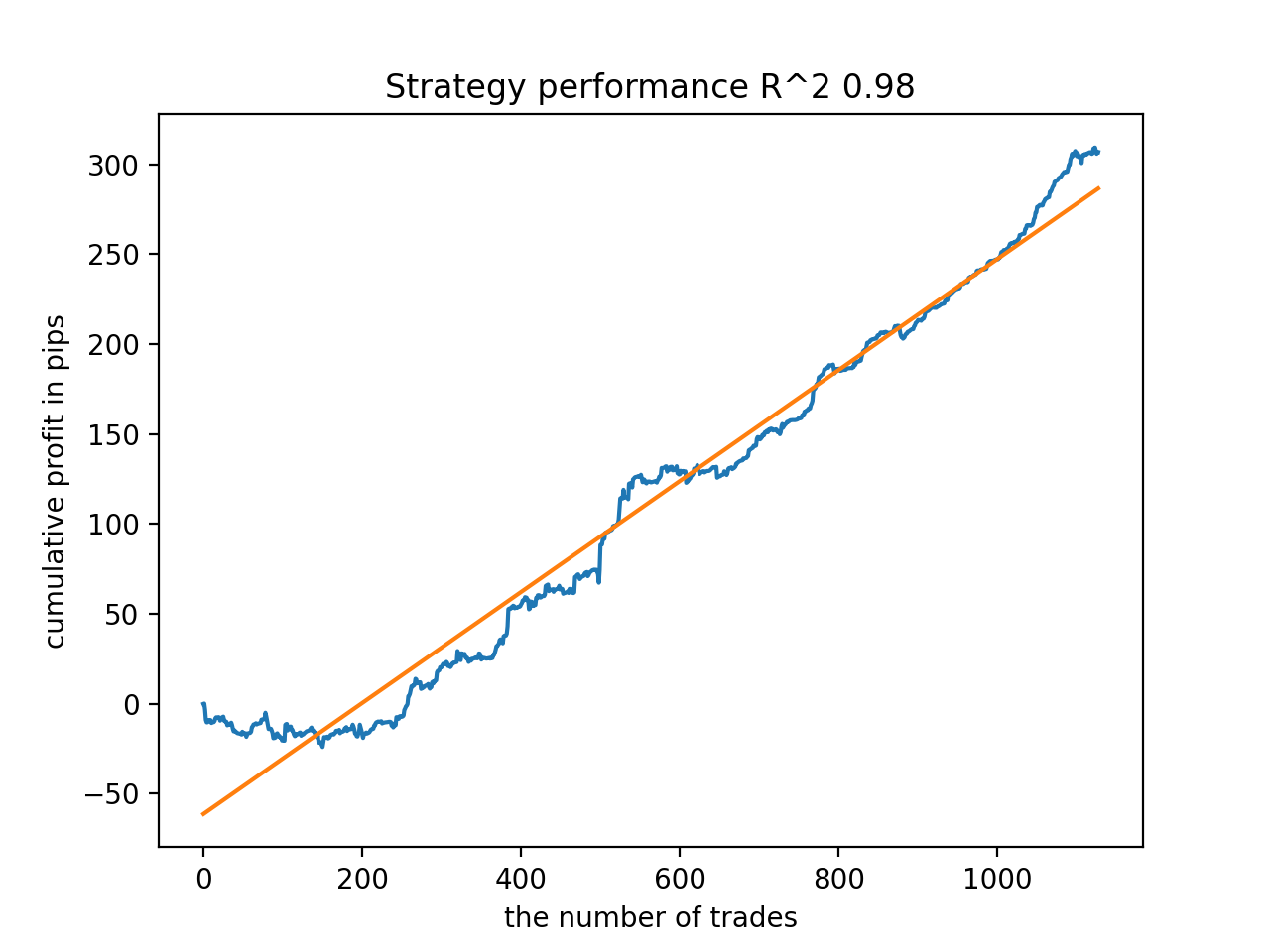
For example, I tested the last trained model and got the following result (all results are based on new data):

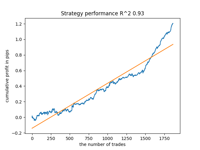
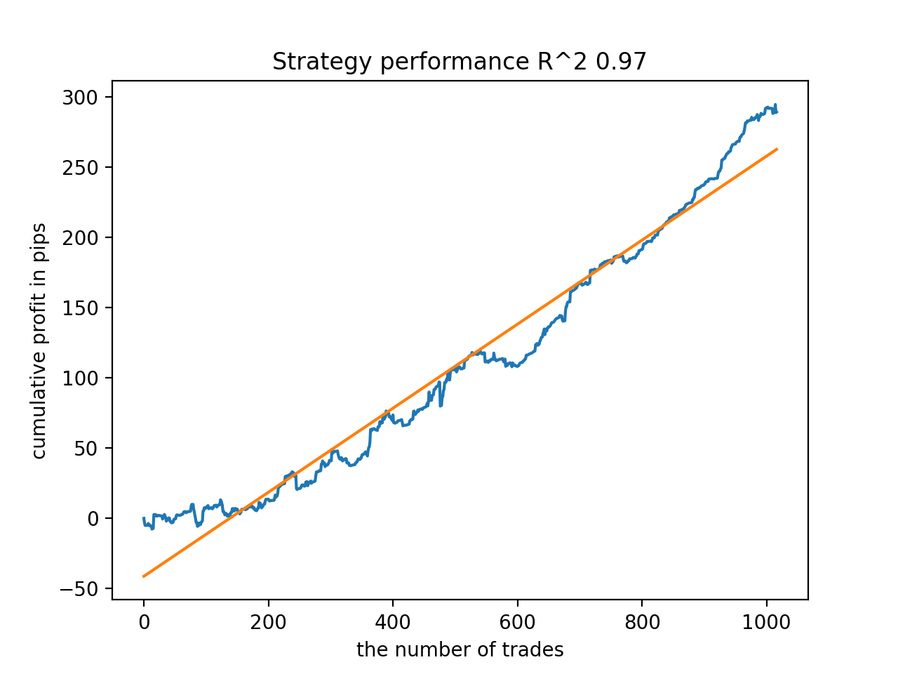
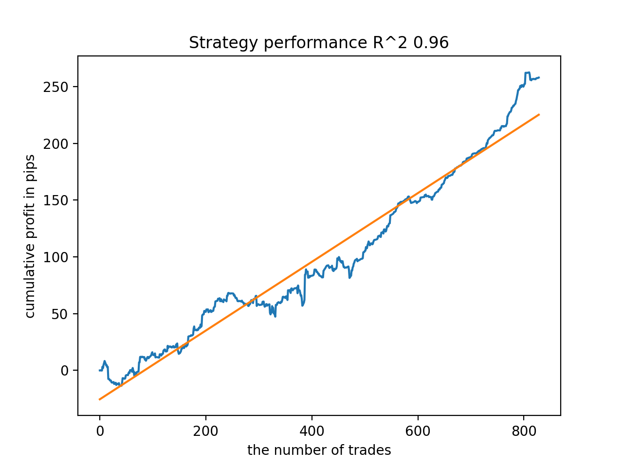
The fifth model from the end will have more deals, and so on:

Depending on the number of iterations and the bad_samples_fraction parameter, as well as on the size of training and test samples, we can get models that are stable on new data. In general, the idea turned out to be working, although quite difficult to understand and implement. Approximately the same situation happened with the enabled use_GMM_resampling parameter. The number of deals directly depends on the number of iterations, but there may be exceptions. I removed resampling from the library as it took too much training time and did not improve results much when applying the approach.

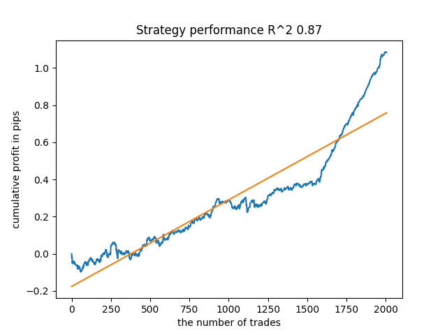
For example, I liked the fifth result from the end:

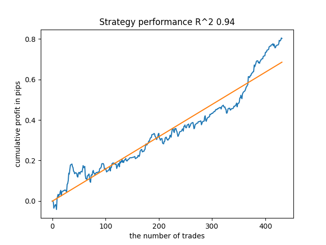
But the seventh result turned out to be preferable in terms of the number of deals, which turned out to be twice as many. The total profit in points also increased:

Exporting models to MQL5 format and compiling a trading EA

The two models are to be saved now: base and metamodel. As before, the base model controls buy and sell signals, while the metamodel prohibits or allows trading at certain points in time.

# add CatBosst base model
    code += 'double catboost_model' + '(const double &features[]) { \n'
    code += '    '
    with open('catmodel.h', 'r') as file:
        data = file.read()
        code += data[data.find("unsigned int TreeDepth")
                               :data.find("double Scale = 1;")]
    code += '\n\n'
    code += 'return ' + \
        'ApplyCatboostModel(features, TreeDepth, TreeSplits , BorderCounts, Borders, LeafValues); } \n\n'

    # add CatBosst meta model
    code += 'double catboost_meta_model' + '(const double &features[]) { \n'
    code += '    '
    with open('meta_catmodel.h', 'r') as file:
        data = file.read()
        code += data[data.find("unsigned int TreeDepth")
                               :data.find("double Scale = 1;")]
    code += '\n\n'
    code += 'return ' + \
        'ApplyCatboostModel(features, TreeDepth, TreeSplits , BorderCounts, Borders, LeafValues); } \n\n'

The trading EA has been slightly changed. The catboost_meta_model() function generating a signal is called. If it exceeds 0.5, then trading is allowed.

void OnTick() {
//---
   if(!isNewBar()) return;
   TimeToStruct(TimeCurrent(), hours);
   double features[];

   fill_arays(features);
   if(ArraySize(features) !=ArraySize(MAs)) {
      Print("No history availible, will try again on next signal!");
      return;
   }
   double sig = catboost_model(features);
   double meta_sig = catboost_meta_model(features);

// close positions by an opposite signal
   if(meta_sig > 0.5)
      if(count_market_orders(0) || count_market_orders(1))
         for(int b = OrdersTotal() - 1; b >= 0; b--)
            if(OrderSelect(b, SELECT_BY_POS) == true) {
               if(OrderType() == 0 && OrderSymbol() == _Symbol && OrderMagicNumber() == OrderMagic && sig > 0.5)
                  if(OrderClose(OrderTicket(), OrderLots(), OrderClosePrice(), 0, Red)) {
                  }
               if(OrderType() == 1 && OrderSymbol() == _Symbol && OrderMagicNumber() == OrderMagic && sig < 0.5)
                  if(OrderClose(OrderTicket(), OrderLots(), OrderClosePrice(), 0, Red)) {
                  }
            }


// open positions and pending orders by signals
   if(meta_sig > 0.5)
      if(countOrders() == 0 && CheckMoneyForTrade(_Symbol,LotsOptimized(),ORDER_TYPE_BUY)) {
         double l = LotsOptimized();

         if(sig < 0.5) {
            OrderSend(Symbol(),OP_BUY,l, Ask, 0, Bid-stoploss*_Point, Ask+takeprofit*_Point, NULL, OrderMagic);

         } else {
            OrderSend(Symbol(),OP_SELL,l, Bid, 0, Ask+stoploss*_Point, Bid-takeprofit*_Point, NULL, OrderMagic);

         }
      }
}

Additions

For MAC and Linux users, the terminal API for loading quotes is not available. I suggest using another function that accepts quotes loaded from the MetaTrader 5 terminal into a file. The file should be saved to the working directory.

def get_prices() -> pd.DataFrame:
    p = pd.read_csv('EURUSDMT5.csv', delim_whitespace=True)
    pFixed = pd.DataFrame(columns=['time', 'close'])
    pFixed['time'] = p['<DATE>'] + ' ' + p['<TIME>']
    pFixed['time'] = pd.to_datetime(pFixed['time'], infer_datetime_format=True)
    pFixed['close'] = p['<CLOSE>']
    pFixed.set_index('time', inplace=True)
    pFixed.index = pd.to_datetime(pFixed.index, unit='s')
    pFixed = pFixed.dropna()
    pFixedC = pFixed.copy()

    count = 0
    for i in MA_PERIODS:
        pFixed[str(count)] = pFixedC - pFixedC.rolling(i).mean()
        count += 1
    return pFixed.dropna()

Three dates are used now. So now it is possible to sort models both by back and forward tests. The start of the forward is set by the STOP_DATE global variable. The data after this date will not be used in training. Instead, it will be used in tests. Similarly, everything before TSTART_DATE is a backtest.

START_DATE = datetime(2021, 1, 1)
TSTART_DATE = datetime(2017, 1, 1)
STOP_DATE = datetime(2022, 1, 1)

Keep in mind that the base model is trained for the START_DATE - STOP_DATE period, while the metamodel is trained on the TSTART_DATE - STOP_DATE data. All other data remaining in the file participates only in back and forward tests.

Some more tests

I decided to test the proposed training method on some cross-rate, for example GBPJPY H1. Quotes from 2010 were downloaded from the terminal. The number of attributes and periods for training are as follows:

MA_PERIODS = [i for i in range(15, 500, 15)]
MARKUP = 0.00002
START_DATE = datetime(2021, 1, 1)
TSTART_DATE = datetime(2018, 1, 1)
STOP_DATE = datetime(2022, 1, 1)

The base model is trained from 2021 to early 2022, while the metamodel is trained from 2018 to 2022. All other data is used for testing on new data, i.e. from 2010 to 2022.06.15.

Sampling of trades with a random duration is selected in the range of 15-35.

def labelling_relabeling(dataset, min=15, max=35, relabeling=False):

25 training iterations are chosen. The multiplier for bad examples for the examples book is equal to 0.5:

# iterative learning
res = []
BAD_SAMPLES_BOOK = pd.DatetimeIndex([])
for i in range(25):
    res.append(brute_force(pr[pr.columns[1:]], bad_samples_fraction=0.5))

    print('Iteration: {}, R^2: {}'.format(i, res[-1][0]))
    pr = res[-1][3] 

# test best model
res.sort()
p = test_model(res[-1])

During training, the following R^2 scores were obtained for the entire dataset since 2010:

Iteration: 0, R^2: 0.8364212812476872
Iteration: 1, R^2: 0.8265960950867208
Iteration: 2, R^2: 0.8710535097094494
Iteration: 3, R^2: 0.820894300254345
Iteration: 4, R^2: 0.7271704621597865
Iteration: 5, R^2: 0.8746302835797399
Iteration: 6, R^2: 0.7746283871087961
Iteration: 7, R^2: 0.870806543378866
Iteration: 8, R^2: 0.8651222653557956
Iteration: 9, R^2: 0.9452164577256995
Iteration: 10, R^2: 0.867541289963404
Iteration: 11, R^2: 0.9759544230548619
Iteration: 12, R^2: 0.9063804006221455
Iteration: 13, R^2: 0.9609701853129079
Iteration: 14, R^2: 0.9666262255426672
Iteration: 15, R^2: 0.7046628448822643
Iteration: 16, R^2: 0.7750941894554821
Iteration: 17, R^2: 0.9436968900331276
Iteration: 18, R^2: 0.8961403809578388
Iteration: 19, R^2: 0.9627553719743711
Iteration: 20, R^2: 0.9559809326980575
Iteration: 21, R^2: 0.9578579606050637
Iteration: 22, R^2: 0.8095556721129047
Iteration: 23, R^2: 0.654147043077418
Iteration: 24, R^2: 0.7538928969905255

Next, the models were sorted by the highest R^2. Here are the best of them in descending order of the score.

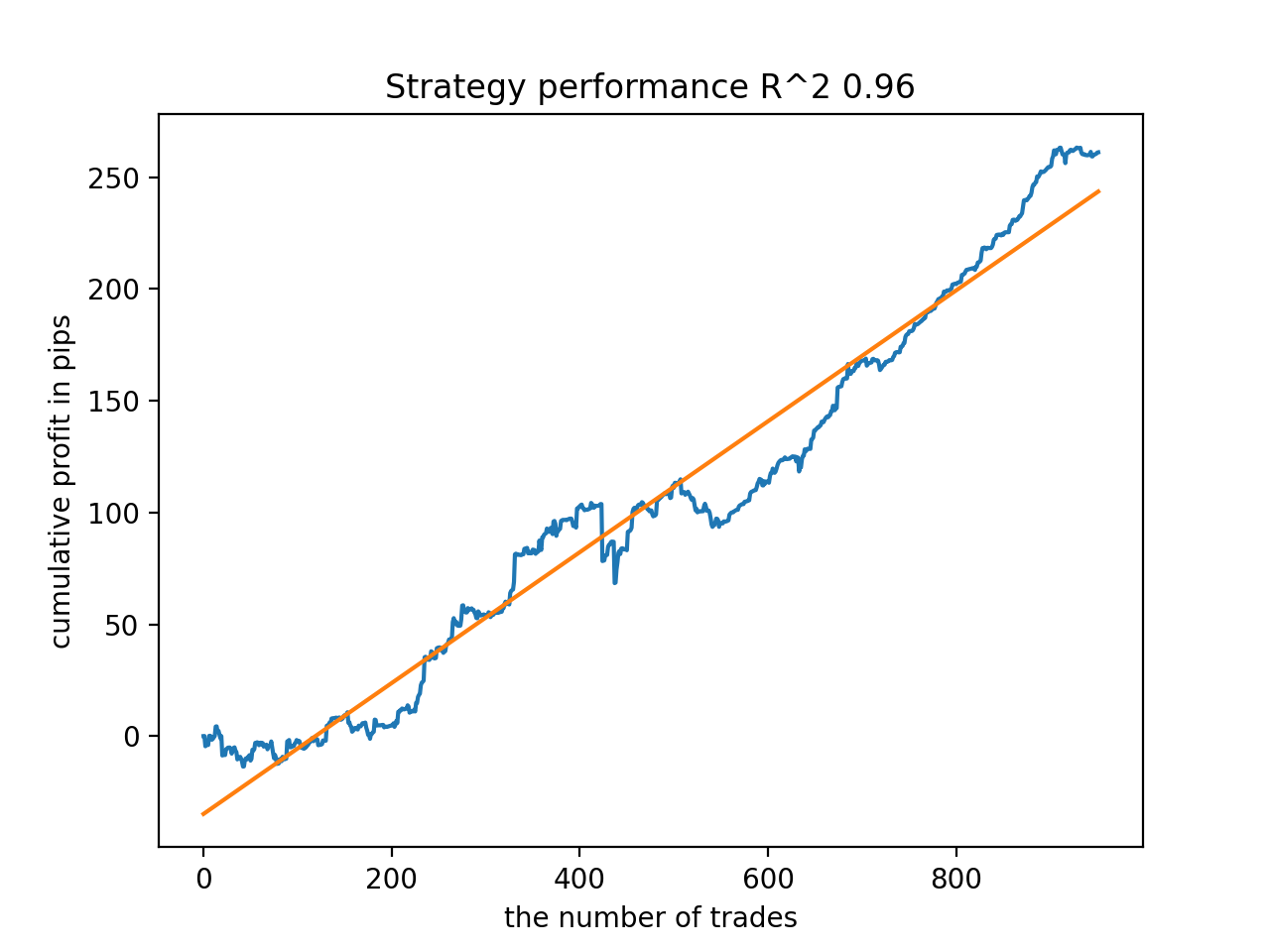
All patterns are generally fairly stable over the period since 2010, although the graphs do not represent perfect curves.

At the final stage, we export the models of interest to MetaTrader 5 for additional tests or use in trading. The export function takes a model as input (in this case, the best from the end) and a model number to change the file name so that you can record several models at the same time.

export_model_to_MQL_code(res[-1], str(1))

Compile the bot and check it in the MetaTrader 5 strategy tester.

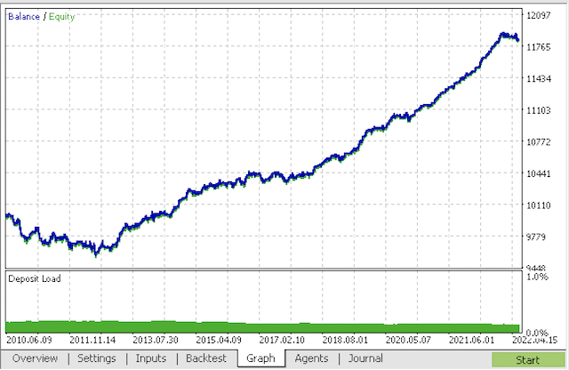
At the final stage, you can already work with models in the familiar MetaTrader 5 terminal.

Conclusion

The article demonstrates probably the most complex and sophisticated time series classification model I have ever had to implement. An interesting point is the ability to automatically discard difficult-to-classify pieces of history using the metamodel. Such models sometimes even outperform seasonal models that have been trained to trade at a specific time of day or at a certain day of the week with strongly pronounced seasonal cycles. Here sorting is performed automatically with no human intervention.