使用机器学习检测与分类分形模式

概述

在第一篇文章中，我们详细探讨了多重分形市场理论的基本方面。我们注意到，在外部信息的影响下，价格图表能够形成某些重复的结构，这些外部信息对价格图表进行了组织。市场参与者创造了一个复杂的动态系统，该系统具有记忆性，并以特定的市场对称结构（模式）的形式表现出来。这些模式可能会随着时间推移而演变，也可能会重复出现。由于分形市场结构的自相似性，模式可以在不同的时间尺度上表达。

本文提出了一种原创性的分形模式识别与分类方法。分析将使用 Python 进行，并能够将最终模型以 ONNX 格式导出到 MetaTrader 5 终端。

开始之前，请确保已安装所有必需的软件包和模块。部分导入模块包含在下方附件中。

import pandas as pd
import math
from datetime import datetime
from catboost import CatBoostClassifier
from sklearn.model_selection import train_test_split
from bots.botlibs.labeling_lib import *
from bots.botlibs.tester_lib import test_model
from bots.botlibs.export_lib import export_model_to_ONNX

分形模式搜索函数的实现

在本文中，我提出了一种通过相关性来寻找对称多重分形市场结构的简单方法。我们可以探索分形和多重分形模式，这两种模式都具有尺度不变性，即它们的大小不同。为此，有必要通过在不同时间尺度上的相关性来执行模式搜索，具体设置将在设置中指定。下面是一个函数，该函数在滑动窗口中计算相关性，同时考虑模式的可变长度。

@njit
def calculate_symmetric_correlation_dynamic(data, min_window_size, max_window_size):
    n = len(data)
    min_w = max(2, min_window_size)
    max_w = max(min_w, max_window_size)
    num_correlations = max(0, n - min_w + 1)

    if num_correlations == 0:
        return np.zeros(0, dtype=np.float64), np.zeros(0, dtype=np.int64)

    correlations = np.zeros(num_correlations, dtype=np.float64)
    best_window_sizes = np.full(num_correlations, -1, dtype=np.int64)

    for i in range(num_correlations):
        max_abs_corr_for_i = -1.0
        best_corr_for_i = 0.0
        current_best_w = -1
        current_max_w = min(max_w, n - i)
        start_w = min_w
        if start_w % 2 != 0:
            start_w += 1

        for w in range(start_w, current_max_w + 1, 2):
            if w < 2 or i + w > n:
                continue
            half_window = w // 2
            window = data[i : i + w]
            first_half = window[:half_window]
            second_half = (window[half_window:] * -1)[::-1]
            
            std1 = np.std(first_half)
            std2 = np.std(second_half)

            if std1 > 1e-9 and std2 > 1e-9:
                mean1 = np.mean(first_half)
                mean2 = np.mean(second_half)
                cov = np.mean((first_half - mean1) * (second_half - mean2))
                corr = cov / (std1 * std2)
                if  abs(corr) > max_abs_corr_for_i:
                    max_abs_corr_for_i = abs(corr)
                    best_corr_for_i =corr
                    current_best_w = w
        
        correlations[i] = best_corr_for_i
        best_window_sizes[i] = current_best_w
        
    return correlations, best_window_sizes

为了加速具有相似计算的循环（在 Python 中循环运行速度较慢），我们使用了 @njit 装饰器，该装饰器通过 Numba 包来加速计算。 

该函数接收收盘价数据作为输入，以及模式的最小和最大“窗口”大小。例如，我们想计算长度为 100 到 200 个 K 线的模式的相关性。然后我们设置好适当的参数，之后针对每个新的起始点和每个给定的模式长度，检查其左侧部分与镜像翻转后的右侧部分之间的相关性。右半部分的反转部分用黄色突出显示。这非常重要，因为我们要寻找数据的对称性。

将每个起始点的最佳绝对相关性的值写入 correlations[] 数组。将与最佳相关性对应的窗口大小（模式长度）写入另一个数组 best_window_sizes[]。因此，该函数会返回每个起始点的最大相关值及其对应的模式。

对发现的模式进行目视检查

一旦计算出所有模式，我们就可以直观地评估算法的正确性。为此，我提出了另一个函数，该函数将显示通过最高绝对皮尔逊相关系数找到的最佳模式。

def plot_best_n_patterns(data, min_window_size, max_window_size, n_best):
    # 1. Calculate correlations and best window sizes
    corrs, window_sizes = calculate_symmetric_correlation_dynamic(data, min_window_size, max_window_size)

    # 2. Find N best patterns
    # Assuming -1 in window_sizes means invalid/not found by the calculation logic
    valid_calc_mask = window_sizes != -1 
    
    if not np.any(valid_calc_mask):
        print("No suitable patterns found (all window sizes were marked as -1 by calculation).")
        return
        
    filtered_corrs = corrs[valid_calc_mask]
    filtered_window_sizes = window_sizes[valid_calc_mask]
    
    original_indices_all = np.arange(len(corrs)) 
    filtered_start_indices = original_indices_all[valid_calc_mask]

    if len(filtered_corrs) == 0: 
        print("No suitable patterns found after filtering out -1 window_sizes.")
        return

    # Sort by absolute correlation value in descending order
    sorted_indices_of_filtered = np.argsort(np.abs(filtered_corrs))[::-1]
    
    # Determine how many of the top patterns to consider
    num_to_consider = min(n_best, len(sorted_indices_of_filtered))

    if num_to_consider == 0:
        print("No patterns to plot (either n_best is too small, or no patterns passed the initial filter).")
        return

    # Pre-filter these top candidates to find those actually plottable (even window size >= 2)
    patterns_to_plot_details = []
    for i in range(num_to_consider):
        idx_in_filtered_arrays = sorted_indices_of_filtered[i] # Index within the already filtered (by valid_calc_mask) arrays
        
        w_best_candidate = filtered_window_sizes[idx_in_filtered_arrays]
        actual_data_start_index = filtered_start_indices[idx_in_filtered_arrays]
        correlation_value = filtered_corrs[idx_in_filtered_arrays]
        
        # Check if the window size is valid for plotting (even and sufficiently large)
        if w_best_candidate >= 2 and w_best_candidate % 2 == 0 : 
            patterns_to_plot_details.append({
                "original_rank_in_consider_list": i, # Rank among the num_to_consider items
                "data_start_index": actual_data_start_index,
                "correlation": correlation_value,
                "window_size": int(w_best_candidate) # Ensure it's int
            })
        else:
            print(f"Info: Top candidate (originally rank {i+1} among considered, "
                  f"Start Index: {actual_data_start_index}) "
                  f"skipped due to invalid window size for plotting: {w_best_candidate} (must be even and >= 2).")


    num_actually_plotted = len(patterns_to_plot_details)

    fig, ax = plt.subplots(1, 1, figsize=(10, 5)) # Single axes for combined plot
    title_fontsize = 12
    label_fontsize = 10
    legend_fontsize = 8
    tick_labelsize = 9

    if num_actually_plotted == 0:
        # This message is shown if, out of the top 'num_to_consider' patterns, none had a valid window size for plotting.
        print("No patterns with valid window sizes (even, >=2) found among the top candidates to display on the chart.")
        ax.text(0.5, 0.5, "No valid patterns to display on the chart.",
                horizontalalignment='center', verticalalignment='center',
                transform=ax.transAxes, fontsize=title_fontsize, color='red')
        ax.set_xticks([])
        ax.set_yticks([])
        fig.suptitle(f"Symmetric Patterns Overlaid", fontsize=title_fontsize) # Generic title
    else:
        # Generate distinct colors for each pattern that will actually be plotted
        plot_colors = plt.cm.viridis(np.linspace(0, 1, num_actually_plotted))

        for plot_idx, pattern_info in enumerate(patterns_to_plot_details):
            actual_data_start_index = pattern_info["data_start_index"]
            correlation_value = pattern_info["correlation"]
            w_best = pattern_info["window_size"]
            
            half_window = w_best // 2
            
            # Ensure indices are within data bounds
            if actual_data_start_index + w_best > len(data):
                print(f"Warning: Pattern P{plot_idx+1} (Idx:{actual_data_start_index}, W:{w_best}) extends beyond data length {len(data)}. Skipping.")
                continue

            left_part_data = data[actual_data_start_index : actual_data_start_index + half_window]
            right_part_data = data[actual_data_start_index + half_window : actual_data_start_index + w_best]
            
            x_indices = np.arange(w_best) # X-axis relative to pattern start
            current_color = plot_colors[plot_idx]

            # Plot left part
            ax.plot(x_indices[:half_window], left_part_data, 
                    color=current_color, linestyle='-', 
                    label=f"P{plot_idx+1} (Idx:{actual_data_start_index}, W:{w_best}, C:{correlation_value:.2f})")
            
            # Plot right part
            ax.plot(x_indices[half_window:], right_part_data, 
                    color=current_color, linestyle='--') 
            
            # Add a vertical line to mark the split point for this pattern
            ax.axvline(x=half_window - 0.5, color=current_color, linestyle=':', linewidth=1, alpha=0.6)

        ax.set_xlabel("Index within Pattern Window", fontsize=label_fontsize)
        ax.set_ylabel("Data Value", fontsize=label_fontsize)
        ax.tick_params(axis='both', which='major', labelsize=tick_labelsize)
        ax.grid(True)
        
        ax.legend(fontsize=legend_fontsize, loc='best')
        # Add a text note to explain line styles
        fig.text(0.99, 0.01, 'Solid: Left Part, Dashed: Right Part (Original)', 
                 horizontalalignment='right', verticalalignment='bottom', 
                 fontsize=legend_fontsize - 1, color='dimgray', transform=fig.transFigure)

        fig.suptitle(f"Top {num_actually_plotted} Symmetric Patterns Overlaid", fontsize=title_fontsize)

    plt.tight_layout(rect=[0, 0.03, 1, 0.96]) # Adjust rect for suptitle and fig.text
    plt.show()

这个函数相当长，但大部分代码都用于处理模式排序和绘图。首先，计算模式本身，然后根据相关系数的值对它们进行排序。确定每个模式在价格历史中的位置，然后进行绘图。该函数的运行结果如下所示。

在第一张图中，我们看到一个被选中的模式具有最高的绝对相关性。它类似于某种局部或全局顶部形态，象征着趋势的逆转。虚线垂直线将该系列分为相等的两半。右半部分进行了符号反转和镜像处理。在此之后，计算左右部分之间的相关性。图表中并未显示经过符号反转后的右半部分，而是展示了原始的报价序列。

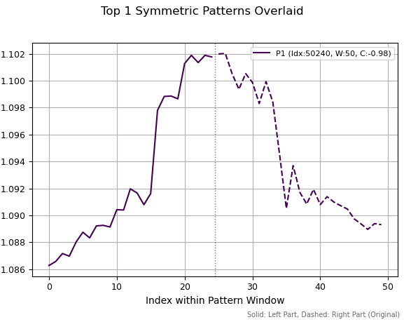
图 1.最佳模式的周期为 50，相关系数为 -0.98

在第二张图中，我展示了周期为 50 的五个最佳模式。在这五个模式中，三个类似于顶部，两个类似于底部；其中一个还看起来像是上涨趋势的延续。左侧刻度显示的是这些形态对应的历史价格水平。

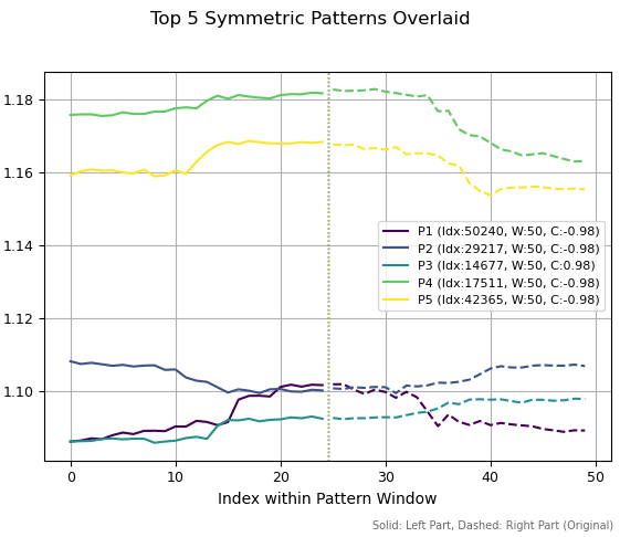
图 2.前五名 50 周期模式

如果我们将模式周期增加到 150 根 K 线，则会观察到完全不同的结构。发现了三个相似的模式（上图）。这是因为在历史数据中的一个轻微时间偏移导致识别出了同一结构。其余两个模式则表现出彼此不同的形态。

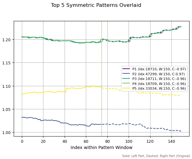
图 3.前五名 150 周期模式

如果我们把模式计算窗口扩大到250，同样的模式再次跻身最佳之列，但历史数据略有变化。也可以观察到一些反转模式，因为它们的相关性为负。

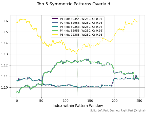
图 4.前五名 250 周期模式

这些图例展示了各种各样的自仿射（即具有某种自相似特征）的市场结构。从理论上讲，这种多样性仅受所研究序列长度的限制。在这种情况下，很难确定哪种特定模式具有预测潜力，哪种没有。研究每个单独的结构需要几个月的时间。机器学习在这方面可以帮到我们，因为它能让我们一次性对所有模式进行分类。

通过相关性来搜索结构很可能并不理想，应考虑采用其他更准确的估计方法。但这种方法为进一步研究提供了良好的起点，且直观易懂。现在我们需要弄清楚如何分析这些市场分形，并利用机器学习基于这些分形构建一个交易系统。

基于对称结构对交易进行标注

从某种意义上说，寻找对称结构的函数是一个数据挖掘函数。我们为在数据中寻找的内容设定了明确的标准 — 自相似的分形结构。接下来，需要对收到的信息进行收集和分类。但即便如此，这仍不够，因为我们必须想出一种方法，根据这些数据来标记交易，而这正是我们将在本节中要做的事情。

我提出以下交易标注方法，以便后续分类。这并非唯一的可能方案，但它反映了作者对如何实施这一方案的理解。我认为需要对这一话题进行更深入的研究，但目前我们将仅限于现有的标记方法。

@njit
def generate_future_outcome_labels_for_patterns(
    close_data_len,                 #  Total length of the original close_data
    correlations_at_window_start,   # Correlation array
    window_sizes_at_window_start,   # Array of window sizes
    source_close_data,              # Full close_data array
    correlation_threshold,
    min_future_horizon,             # Minimum horizon for determining the future price
    max_future_horizon,             # Maximum horizon
    markup_points                   # "Markup" for determining a significant price change
):
    labels = np.full(close_data_len, 2.0, dtype=np.float64)  # 2.0: no signal/neutral/no pattern
    num_potential_windows = len(correlations_at_window_start)

    for idx_window_start in range(num_potential_windows):
        corr_value = correlations_at_window_start[idx_window_start]
        w = window_sizes_at_window_start[idx_window_start]

        # Condition 1: The correlation should be strong enough
        if abs(corr_value) < correlation_threshold:
            continue

        # Condition 2: A valid window should be found
        if w < 2:
            continue

        # The point in time (index) when the correlation pattern is fully formed
        signal_time_idx = idx_window_start + w - 1

        if signal_time_idx >= close_data_len: # Theoretically, this should not happen
            continue
            
        # Array for storing labels for the entire pattern (both left and right parts)
        pattern_labels = []
            
        # Calculate individual marks for all points of the pattern
        for point_idx in range(idx_window_start, signal_time_idx + 1):
            # Current price for this particular point
            current_price = source_close_data[point_idx]
            
            # Define the forecast horizon
            current_horizon = min_future_horizon
            if max_future_horizon > min_future_horizon:
                current_horizon = random.randint(min_future_horizon, max_future_horizon)
            
            # Index of future price relative to the current point
            future_price_idx = point_idx + current_horizon
            
            if future_price_idx >= close_data_len:
                continue
                
            future_price = source_close_data[future_price_idx]
            
            # Define a label for the current point
            current_label = 2.0  # Neutral by default
            if future_price > current_price + markup_points:
                current_label = 0.0  # Price increased
            elif future_price < current_price - markup_points:
                current_label = 1.0  # Price fell
                
            # Add the label to the array if it is not neutral
            if current_label != 2.0:
                pattern_labels.append(current_label)
        
        # If there are no significant marks in the pattern, move on to the next pattern
        if len(pattern_labels) == 0:
            continue
            
        # Calculate the average mark for all points of the pattern
        avg_label = 0.0
        for l in pattern_labels:
            avg_label += l
        avg_label /= len(pattern_labels)
        
        # Define a common label for the entire pattern
        pattern_label = 0.0 if avg_label < 0.5 else 1.0
        
        # Assign this label to all points of the pattern
        for i in range(idx_window_start, signal_time_idx + 1):
            labels[i] = pattern_label
        
    return labels

generate_future_outcome_labels_for_patterns() 函数实现了以下功能：

• 输入是原始价格数组、相关系数数组以及与特定数据点的最大相关系数相对应的模式长度数组。该函数还接受以 K 线数量表示的最小和最大预测范围。
• 最初，所有样本初始都标记为 2.0（不交易）。
• 循环检查时间序列中每个点的相关值。如果相关性超过 correlation_threshhold，则此观测值将进行额外处理，否则此示例的标签将保持为 2.0。
• 然后，在整个模式长度内（通过最大相关性确定），根据未来的价格变化计算交易。对于每个点：如果价格上涨，则此点为 0 - 买入；如果价格下跌，则此点为 1 - 卖出。计算所有交易的平均值，并为当前模式的每个观测值分配一个平均分数。

这种方法背后的理念是，高度相关的结构对其初始条件具有“记忆”，并表现出一定程度的规律性。这意味着其中的观测值预测效果更好，但为了防止过拟合，我们为每个观测值赋予一个平均标签。相反，低相关性结构中的观测值预测效果较差，因为它们的规律性较弱。

因此，我们遵循以下原则：一个模型将决定模式的质量（即当前是否值得交易），另一个模型将决定交易的方向。机器学习的任务是近似预测所有可能的模式和交易方向。

接下来，我们需要另一个调度函数，该函数将直接用于标记交易。

最终的基于分形模式的标记函数

现在是时候将所有内容整合起来，编写一个可直接使用的交易标签工具了。 

def get_fractal_pattern_labels_from_future_outcome(
    dataset,
    min_window_size=6,
    max_window_size=60,
    correlation_threshold=0.7,
    min_future_horizon=5, 
    max_future_horizon=5,    
    markup_points=0.00010,  
):
    if 'close' not in dataset.columns:
        raise ValueError("Dataset must contain a 'close' column.")

    close_data = dataset['close'].values
    n_data = len(close_data)

    if min_window_size < 2:
        min_window_size = 2
    if max_window_size < min_window_size:
        max_window_size = min_window_size
    if min_future_horizon <= 0:
        raise ValueError("min_future_horizon must be > 0")
    if max_future_horizon < min_future_horizon:
        raise ValueError("max_future_horizon must be >= min_future_horizon")
    
    correlations_at_start, best_window_sizes_at_start = calculate_symmetric_correlation_dynamic(
        close_data,
        min_window_size,
        max_window_size,
    )

    labels = generate_future_outcome_labels_for_patterns(
        n_data,
        correlations_at_start,
        best_window_sizes_at_start,
        close_data,
        correlation_threshold,
        min_future_horizon,
        max_future_horizon,
        markup_points
    )

    result_df = dataset.copy()
    result_df['labels'] = pd.Series(labels, index=dataset.index)    
    return result_df

直接调用 get_fractal_pattern_labels_from_future_outcome() 函数来标记您的数据集：

• 输入是一个数据帧，其中应包含一个 “close” 列，其中包含收盘价，以及特征（可选）；
• 已设定用于标记交易的模式的最小和最大长度；
• 设定一个相关性阈值，这使我们能够调整标记中所涉及模式的“准确性”；
• 还应规定标记交易的最小和最大持仓时间（以 K 线数表示）；
• 我们可以选择性地设置标记。

该函数接收一个收盘价数据集，并根据分形模式为交易打上标签，同时添加一个包含已标记标记的 “labels” 列。

基于分形标记训练机器学习模型

现在，所有实验准备工作都已就绪，你可以开始训练模型了。我以 2010 年至今的 EURUSD 小时报价作为数据来源。

决定使用不同时段滑动窗口中的标准差作为特征：

def get_features(data: pd.DataFrame) -> pd.DataFrame:
    pFixed = data.copy()
    pFixedC = data.copy()
    count = 0

    for i in hyper_params['periods']:
        pFixed[str(count)] = pFixedC.rolling(i).std()
        count += 1

    return pFixed.dropna()

接下来，你需要正确设置模型超参数：

# set hyper parameters
hyper_params = {
    'symbol': 'EURUSD_H1',
    'export_path': '/Users/dmitrievsky/Library//drive_c/Program Files/MetaTrader 5/MQL5/Include/Trend following/',
    'model_number': 0,
    'markup': 0.00010,
    'stop_loss':  0.00500,
    'take_profit': 0.00500,
    'periods': [i for i in range(15, 300, 30)],
    'backward': datetime(2010, 1, 1),
    'forward': datetime(2024, 1, 1),
}

• 止损和止盈相同，均为 500 个五位小数点；
• 接下来，我们需要指定将训练好的模型导出到我们文件夹的路径；
• 我们将特征周期（标准差）的范围设置为 15 到 300，步长为 30（总共有 10 个特征）；
• 训练期为 2010 年至 2024 年，其余数据不在训练范围内。

主训练循环允许同时训练多个模型，并且还允许对超参数进行迭代：

# fit the models
models = []
for i in range(10):
    print('Learn ' + str(i) + ' model')
    dataset = get_features(get_prices())
    data = dataset[(dataset.index < hyper_params['forward']) & (dataset.index > hyper_params['backward'])].copy()
    data = get_fractal_pattern_labels_from_future_outcome(data, 100, 100, 0.9, 15, 25, 0.00010)
    models.append(fit_final_models(data))

在循环中，我们首先获取价格和特性，然后确定模型训练的时间周期。

在 get_fractal_pattern_labels_from_future_outcome() 函数中，传递以下参数：

• 包含价格和特征的原始数据帧
• 计算相关性的最小窗口
• 计算相关性的最大窗口
• 模式相关系数阈值，默认值为 0.9
• 最小预测范围（以 K 线数为单位）
• 最大预测范围（以 K 线数为单位）
• 价格变动阈值

然后，将标记好的数据输入到一个函数中，该函数会训练两个分类器：

def fit_final_models(dataset: pd.DataFrame) -> list:
    feature_columns = dataset.columns[1:-1]

    # 1. Data for the main model
    # Filter the dataset: only those examples where 'labels' are equal to 0 or 1 are used for the main model.
    main_model_df = dataset[dataset['labels'].isin([0, 1])].copy()
    
    X = main_model_df[feature_columns]
    y = main_model_df['labels'].astype('int16')

    # 2. Data for the meta model
    X_meta = dataset[feature_columns]
    
    # Modify labels for the meta model: if 'labels' contains 1 or 0, then the new label is 1, if 2, then 0.
    y_meta = dataset['labels'].apply(lambda label_val: 1 if label_val in [0, 1] else 0).astype('int16')

    # For the main model
    train_X, test_X, train_y, test_y = train_test_split(
        X, y, train_size=0.7, test_size=0.3, shuffle=True) 
    
    # For the meta model
    train_X_m, test_X_m, train_y_m, test_y_m = train_test_split(
        X_meta, y_meta, train_size=0.7, test_size=0.3, shuffle=True)
    
    # Train the main model
    model = CatBoostClassifier(iterations=1000,
                               custom_loss=['Accuracy'],
                               eval_metric='Accuracy',
                               verbose=False,
                               use_best_model=True,
                               task_type='CPU',
                               )
    
    # Check if the samples are empty after splitting (unlikely if X is large enough)
    if not train_X.empty and not test_X.empty:
        model.fit(train_X, train_y, eval_set=(test_X, test_y),
                  early_stopping_rounds=25, plot=False)
    elif not train_X.empty: # If the test sample is empty, but the training sample exists
        print("Warning: The test sample (test_X) for the main model is empty. The model is trained without eval_set.")
        model.fit(train_X, train_y, early_stopping_rounds=15, plot=False) # use_best_model may not work correctly without eval_set
    else: # If the training set is empty
        print("Error: The training set (train_X) for the main model is empty. The model cannot be trained.")
        # In this case, test_model will most likely throw an error later.
        # Return R2=-1 and the untrained model, the meta model will also not make sense without the main one.
        print("R2 is fixed at -1.0, models are not trained.")
        return [-1.0, model, None] # model - instance, but not trained

    # Meta model training
    meta_model = CatBoostClassifier(iterations=1000,
                                    custom_loss=['F1'],
                                    eval_metric='F1',
                                    verbose=False,
                                    use_best_model=True,
                                    task_type='CPU',
                                    )

    if not train_X_m.empty and not test_X_m.empty:
        meta_model.fit(train_X_m, train_y_m, eval_set=(test_X_m, test_y_m),
                       early_stopping_rounds=25, plot=False)
    elif not train_X_m.empty:
        print("Warning: The test sample (test_X_m) for the meta model is empty. The meta model is trained without eval_set.")
        meta_model.fit(train_X_m, train_y_m, early_stopping_rounds=25, plot=False)
    else:
        print("Error: The training set (train_X_m) for the meta model is empty. The meta model cannot be trained.")
        print("R2 fixed as -1.0.")
        return [-1.0, model, meta_model] # meta_model - instance, but not trained

    data_for_test = get_features(get_prices())
    R2 = test_model(data_for_test, 
                    [model, meta_model], 
                    hyper_params['stop_loss'], 
                    hyper_params['take_profit'],
                    hyper_params['forward'],
                    hyper_params['backward'],
                    hyper_params['markup'],
                    plt=False)
    
    if math.isnan(R2):
        R2 = -1.0
        print('R2 fixed as -1.0')
    print('R2: ' + str(R2))
    result = [R2, model, meta_model]
    return result

值得特别注意的点已用粗体突出显示。主模型仅训练用于预测 0 或 1 标签，而附加的元模型则用于预测是否进行交易。

测试和最终结果

首先值得一提的是，我只在 EURUSD 货币对上测试了该算法。我能够选择最适合新数据的模式窗口大小。它等于100。算法的最优参数已在代码中指定，因此您可以自行复现结果。

训练数据和测试数据的资金曲线如下所示：

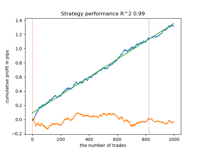
图 5.测试基于分形标记的算法

相关阈值与新数据上的交易结果之间存在直接关系。例如，当阈值为 0.7 时，资金曲线已经显示出明显的过拟合现象。这反映了时间序列中两个部分之间的弱相关性会导致弱依赖性的事实。而弱依赖性则无法对可靠模式进行正确分类，因为它们与不可靠模式混杂在一起。

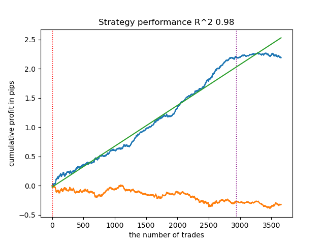
图 6.使用阈值 0.7 对算法进行测试

正确识别模式似乎至关重要。关于如何最好地组织对分形结构的搜索，还需要进一步的研究和深入见解。

特征的质量和数量也会影响分类结果。如果我们使用增量而不是标准差，资金曲线将会呈现出不同的形态。

同样有必要对基于所发现的模式对交易进行标记的方法进行分析和合理批判。

CatBoost 模型的误差分析表明，这些模型训练误差较低：

>>> models[-1][1].get_best_score()['validation']
{'Accuracy': 0.9700523560209424, 'Logloss': 0.17002244404784328}
>>> models[-1][2].get_best_score()['validation']
{'Logloss': 0.25629795409043277, 'F1': 0.8455473098330242}
>>> 

在 MetaTrader 5 终端中导出和测试模型

要导出模型，我们需要调用以下函数：

export_model_to_ONNX(model = models[-1],
                     symbol = hyper_params['symbol'],
                     periods = hyper_params['periods'],
                     periods_meta = hyper_params['periods'],
                     model_number = hyper_params['model_number'],
                     export_path = hyper_params['export_path'])

导出并编译 EA 后，我们得到了以下结果：

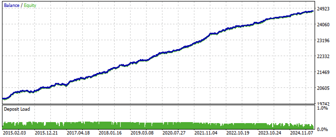
图 7.在整个期间内测试 EA

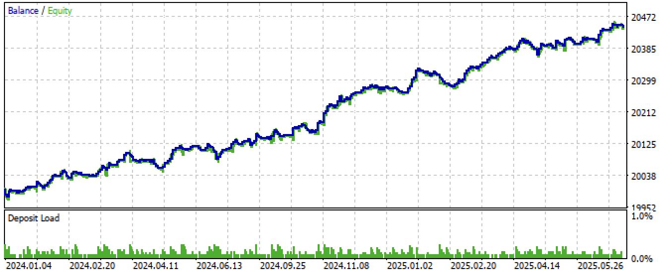
图 8.在新数据上测试 EA

结论

在本文中，我们探讨了利用机器学习进行分形分析和市场预测这一有趣的话题。这只是迈向探索金融价格图表上形成的各种分形结构的最初几步。

需要注意的是，相关性搜索可能无法完全反映过去和未来价格序列之间的关系，这一课题有待进一步研究。例如，回归分析可能比相关性分析更合适。同时，当前算法在配置得当的情况下能够展现出良好的预测能力，这证实了金融时间序列中存在分形自相似结构。

Python files.zip 压缩包包含以下用于 Python 开发环境的文件：

文件名	描述
fractal patterns.py	用于训练模型的主脚本
labeling_lib.py	更新后的交易标签模块
tester_lib.py	基于机器学习的更新版自定义策略测试器
export_lib.py	用于将模型导出到终端的模块
EURUSD_H1.csv	从 MetaTrader 5 导出的报价数据

MQL5 files.zip 压缩包包含 MetaTrader 5 终端所需的文件：

文件名	描述
fractal trader.ex5	文章中编译的机器人
fractal trader.mq5	文章中的机器人源代码
Include/Trend following 文件夹	ONNX 模型和用于连接机器人的头文件。