Neural networks made easy (Part 7): Adaptive optimization methods

Contents

• Introduction
• 1. Distinctive features of adaptive optimization methods
• 1.1. Adaptive Gradient Method (AdaGrad)
• 1.2. RMSProp method
• 1.3. Adadelta Method
• 1.4. Adaptive Moment Estimation Method (Adam)
• 2. Implementation
• 2.1. Building the OpenCL kernel
• 2.2. Changes in the code of the main program's neuron class
• 2.3. Changes in the code of class not using OpenCL
• 2.4. Changes in the code of the main program's neural network class
• 3. Testing
• Conclusions
• References
• Programs used in the article

Introduction

In previous articles, we used different types of neurons, but we always used stochastic gradient descent to train the neural network. This method can probably be called basic, and its variations are very often used in practice. However, there are a lot of other neural network training methods. Today I propose considering adaptive learning methods. This family of methods enables changing of neuron learning rate during neural network training.

1. Distinctive features of adaptive optimization methods

You know that not all features fed into a neural network have the same effect on the final result. Some parameters can contain a lot of noise and can change more often than others, with different amplitudes. Samples of other parameters may contain rare values which can be unnoticed when training the neural network with a fixed learning rate. One of the disadvantages of the previously considered stochastic gradient descent method is the unavailability of optimization mechanisms on such samples. As a result, the learning process can stop at a local minimum. This problem can be solved using adaptive methods for training neural networks. These methods allow the dynamic change of the learning rate in the neural network training process. There are a number of such methods and their variations. Let us consider the most popular of them.

1.1. Adaptive Gradient Method (AdaGrad)

The Adaptive Gradient Method was proposed in 2011. It is a variation to the stochastic gradient descent method. By comparing the mathematical formulas of these methods, we can easily notice one difference: the learning rate in AdaGrad is divided by the square root of the sum of the squares of gradients for all previous training iterations. This approach allows reducing the learning rate of frequently updated parameters.

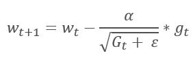
The main disadvantage of this method follows from its formula: the sum of the squares of the gradients can only grow and thus, the learning rate tends to 0. This will ultimately cause the training to stop.

The utilization of this method requires additional calculations and allocation of additional memory to store the sum of squares of gradients for each neuron.

1.2. RMSProp method

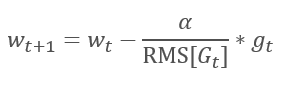
The logical continuation of the AdaGrad method is the RMSProp method. To avoid the dropping of the learning rate to 0, the sum of the squares of past gradients has been replaced by the exponential mean of the squared gradients in the denominator of the formula used for updating the weights. This approach eliminates the constant and infinite growth of the value in the denominator. Furthermore, it gives greater attention to the latest values of the gradient that characterize the current state of the model. 

1.3. Adadelta Method

The Adadelta adaptive method was proposed almost simultaneously with RMSProp. This method is similar and it uses an exponential mean of the sum of squared gradients in the denominator of the formula used for updating the weights. But unlike RMSProp, this method completely refuses the learning rate in the update formula and replaces it with an exponential mean of the sum of squares of previous changes in the analyzed parameter.

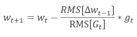
This approach allows removing the learning rate from the formula used for updating the weights, and to create a highly adaptive learning algorithm. However, this method requires additional iterations of calculations and allocation of memory for storing an additional value in each neuron.

1.4. Adaptive Moment Estimation Method (Adam)

In 2014, Diederik P. Kingma and Jimmy Lei Ba proposed the Adaptive Moment Estimation Method (Adam). According to the authors, the method combines the advantages of the AdaGrad and RMSProp methods and it works well for on-line training. This method shows consistently good results on different samples. It is often recommended for use by default in various packages.

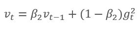
The method is based on the calculation of the exponential average of gradients m and the exponential average of squared gradients v. Each exponential average has its own hyperparameter ß which determines the averaging period.

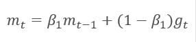
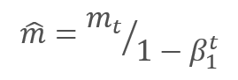
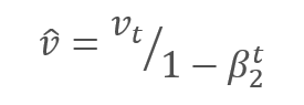
The authors suggest the default use of ß1 at 0.9 and ß2 at 0.999. In this case m0 and v0 take zero values. With these parameters, the formulas presented above return values close to 0 at the beginning of training, and thus the learning rate at the beginning will be low. To speed up the learning process, the authors suggest correcting the obtained moment.

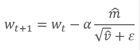
The parameters are updated by adjusting for the ratio of the corrected gradient moment m to the square root of the corrected moment of the squared gradient v. To avoid dividing by zero, the Ɛ constant close to 0 is added to the denominator. The resulting ratio is adjusted by the learning factor α, which in this case is the upper bound of the learning step. The authors suggest using α at 0.001 by default.

2. Implementation

After considering the theoretical aspects, we can proceed to practical implementation. I propose to implement the Adam method with the default hyperparameters offered by the authors. Further you can try other variations of hyperparameters.

The earlier built neural network used stochastic gradient descent for training, for which we have already implemented the back propagation algorithm. The existing back propagation functionality can be used to implement the Adam method. We only need to implement the weight updating algorithm. This functionality is performed by the updateInputWeights method, which is implemented in each class of neurons. Of course, we will not delete the previously created stochastic gradient descent algorithm. Let us create an alternative algorithm enabling the choice of the training method to be used.

2.1. Building the OpenCL kernel

Consider the implementation of the Adam method for the CNeuronBaseOCL class. First, create the UpdateWeightsAdam kernel to implement the method in OpenCL. Pointers to the following matrices will be passed to the kernel in parameters:

• matrix of weights — matrix_w,
• matrix of error gradients  — matrix_g,
• input data matrix — matrix_i,
• matrix of exponential means of gradients — matrix_m,
• matrix of exponential means of squared gradients   — matrix_v.

__kernel void UpdateWeightsAdam(__global double *matrix_w,
                                __global double *matrix_g,
                                __global double *matrix_i,
                                __global double *matrix_m,
                                __global double *matrix_v,
                                int inputs, double l, double b1, double b2)

Additionally, in the kernel parameters, pass the size of the input data array and the hyperparameters of the Adam algorithm.

At the kernel beginning, obtain the serial numbers of the stream in two dimensions, which will indicate the numbers of the neurons of the current and previous layers, respectively. Using the received numbers, determine the initial number of the processed element in the buffers. Pay attention that the resulting stream number in the second dimension is multiplied by "4". This is because in order to reduce the number of streams and the total program execution time, we will use vector calculations with 4-element vectors.

  {
   int i=get_global_id(0);
   int j=get_global_id(1);
   int wi=i*(inputs+1)+j*4;

After determining the position of the processed elements in data buffers, declare vector variables and fill them with the corresponding values. Use the previously described method and fill the missing data in vectors with zeros.

   double4 m, v, weight, inp;
   switch(inputs-j*4)
     {
      case 0:
        inp=(double4)(1,0,0,0);
        weight=(double4)(matrix_w[wi],0,0,0);
        m=(double4)(matrix_m[wi],0,0,0);
        v=(double4)(matrix_v[wi],0,0,0);
        break;
      case 1:
        inp=(double4)(matrix_i[j],1,0,0);
        weight=(double4)(matrix_w[wi],matrix_w[wi+1],0,0);
        m=(double4)(matrix_m[wi],matrix_m[wi+1],0,0);
        v=(double4)(matrix_v[wi],matrix_v[wi+1],0,0);
        break;
      case 2:
        inp=(double4)(matrix_i[j],matrix_i[j+1],1,0);
        weight=(double4)(matrix_w[wi],matrix_w[wi+1],matrix_w[wi+2],0);
        m=(double4)(matrix_m[wi],matrix_m[wi+1],matrix_m[wi+2],0);
        v=(double4)(matrix_v[wi],matrix_v[wi+1],matrix_v[wi+2],0);
        break;
      case 3:
        inp=(double4)(matrix_i[j],matrix_i[j+1],matrix_i[j+2],1);
        weight=(double4)(matrix_w[wi],matrix_w[wi+1],matrix_w[wi+2],matrix_w[wi+3]);
        m=(double4)(matrix_m[wi],matrix_m[wi+1],matrix_m[wi+2],matrix_m[wi+3]);
        v=(double4)(matrix_v[wi],matrix_v[wi+1],matrix_v[wi+2],matrix_v[wi+3]);
        break;
      default:
        inp=(double4)(matrix_i[j],matrix_i[j+1],matrix_i[j+2],matrix_i[j+3]);
        weight=(double4)(matrix_w[wi],matrix_w[wi+1],matrix_w[wi+2],matrix_w[wi+3]);
        m=(double4)(matrix_m[wi],matrix_m[wi+1],matrix_m[wi+2],matrix_m[wi+3]);
        v=(double4)(matrix_v[wi],matrix_v[wi+1],matrix_v[wi+2],matrix_v[wi+3]);
        break;
     }

The gradient vector is obtained by multiplying the gradient of the current neuron by the input data vector.

   double4 g=matrix_g[i]*inp;

Next, calculate the exponential averages of the gradient and the squared gradient.

   double4 mt=b1*m+(1-b1)*g;
   double4 vt=b2*v+(1-b2)*pow(g,2)+0.00000001;

Calculate parameter change deltas.

   double4 delta=l*mt/sqrt(vt);

Note that we have not adjusted the received moments in the kernel. This step is intentionally omitted here. Since ß1 and ß2 are the same for all neurons, and t, which is here the number of iterations of neuron parameter updates, is also the same for all neurons, then the correction factor will also be the same for all neurons. That is why we will not recalculate the factor for each neuron but will calculate it once in the main program code and will pass to the kernel the learning coefficient adjusted by this value.

After calculating the deltas, we only need to adjust the weight coefficients and to update the calculated moments in buffers. Then exit the kernel.

   switch(inputs-j*4)
     {
      case 2:
        matrix_w[wi+2]+=delta.s2;
        matrix_m[wi+2]=mt.s2;
        matrix_v[wi+2]=vt.s2;
      case 1:
        matrix_w[wi+1]+=delta.s1;
        matrix_m[wi+1]=mt.s1;
        matrix_v[wi+1]=vt.s1;
      case 0:
        matrix_w[wi]+=delta.s0;
        matrix_m[wi]=mt.s0;
        matrix_v[wi]=vt.s0;
        break;
      default:
        matrix_w[wi]+=delta.s0;
        matrix_m[wi]=mt.s0;
        matrix_v[wi]=vt.s0;
        matrix_w[wi+1]+=delta.s1;
        matrix_m[wi+1]=mt.s1;
        matrix_v[wi+1]=vt.s1;
        matrix_w[wi+2]+=delta.s2;
        matrix_m[wi+2]=mt.s2;
        matrix_v[wi+2]=vt.s2;
        matrix_w[wi+3]+=delta.s3;
        matrix_m[wi+3]=mt.s3;
        matrix_v[wi+3]=vt.s3;
        break;
     }
  };

This code has another trick. Pay attention to the reverse order of case cases in the switch operator. Also, the break operator is only used after case 0 and default case. This approach allows avoiding the duplication of same code for all variants.

2.2. Changes in the code of the main program's neuron class

After building the kernel, we need to make changes to the main program code. First, add constants to the 'define' block for working with the kernel.

#define def_k_UpdateWeightsAdam   4
#define def_k_uwa_matrix_w        0
#define def_k_uwa_matrix_g        1
#define def_k_uwa_matrix_i        2
#define def_k_uwa_matrix_m        3
#define def_k_uwa_matrix_v        4
#define def_k_uwa_inputs          5
#define def_k_uwa_l               6
#define def_k_uwa_b1              7
#define def_k_uwa_b2              8

Create enumerations to indicate training methods and add moment buffers to enumerations.

enum ENUM_OPTIMIZATION
  {
   SGD,
   ADAM
  };
//---
enum ENUM_BUFFERS
  {
   WEIGHTS,
   DELTA_WEIGHTS,
   OUTPUT,
   GRADIENT,
   FIRST_MOMENTUM,
   SECOND_MOMENTUM
  };

Then, in the CNeuronBaseOCL class body, add buffers for storing moments, exponential average constants, training iterations counter and a variable for storing the training method.

class CNeuronBaseOCL    :  public CObject
  {
protected:
   .........
   .........
   ..........
   CBufferDouble     *FirstMomentum;
   CBufferDouble     *SecondMomentum;
//---
   .........
   .........
   const double      b1;
   const double      b2;
   int               t;
//---
   .........
   .........
   ENUM_OPTIMIZATION optimization;

In the class constructor, set the values of the constants and initialize the buffers.

CNeuronBaseOCL::CNeuronBaseOCL(void)   :  alpha(momentum),
                                          activation(TANH),
                                          optimization(SGD),
                                          b1(0.9),
                                          b2(0.999),
                                          t(1)
  {
   OpenCL=NULL;
   Output=new CBufferDouble();
   PrevOutput=new CBufferDouble();
   Weights=new CBufferDouble();
   DeltaWeights=new CBufferDouble();
   Gradient=new CBufferDouble();   
   FirstMomentum=new CBufferDouble();   
   SecondMomentum=new CBufferDouble();   
  }

Do not forget to add the deletion of buffer objects in the class destructor.

CNeuronBaseOCL::~CNeuronBaseOCL(void)
  {
   if(CheckPointer(Output)!=POINTER_INVALID)
      delete Output;
   if(CheckPointer(PrevOutput)!=POINTER_INVALID)
      delete PrevOutput;
   if(CheckPointer(Weights)!=POINTER_INVALID)
      delete Weights;
   if(CheckPointer(DeltaWeights)!=POINTER_INVALID)
      delete DeltaWeights;
   if(CheckPointer(Gradient)!=POINTER_INVALID)
      delete Gradient;
   if(CheckPointer(FirstMomentum)!=POINTER_INVALID)
      delete FirstMomentum;
   if(CheckPointer(SecondMomentum)!=POINTER_INVALID)
      delete SecondMomentum;
   OpenCL=NULL;
  }

In the parameters of the class initialization function, add a training method and, depending on the specified training method, initialize the buffers. If stochastic gradient descent is used for training, initialize the buffer of deltas and remove the biffers of moments. If the Adam method is used, initialize the moment buffers and delete the buffer of deltas.

bool CNeuronBaseOCL::Init(uint numOutputs,uint myIndex,COpenCLMy *open_cl,uint numNeurons, ENUM_OPTIMIZATION optimization_type)
  {
   if(CheckPointer(open_cl)==POINTER_INVALID || numNeurons<=0)
      return false;
   OpenCL=open_cl;
   optimization=optimization_type;
//---
   ....................
   ....................
   ....................
   ....................
//---
   if(numOutputs>0)
     {
      if(CheckPointer(Weights)==POINTER_INVALID)
        {
         Weights=new CBufferDouble();
         if(CheckPointer(Weights)==POINTER_INVALID)
            return false;
        }
      int count=(int)((numNeurons+1)*numOutputs);
      if(!Weights.Reserve(count))
         return false;
      for(int i=0;i<count;i++)
        {
         double weigh=(MathRand()+1)/32768.0-0.5;
         if(weigh==0)
            weigh=0.001;
         if(!Weights.Add(weigh))
            return false;
        }
      if(!Weights.BufferCreate(OpenCL))
         return false;
   //---
      if(optimization==SGD)
        {
         if(CheckPointer(DeltaWeights)==POINTER_INVALID)
           {
            DeltaWeights=new CBufferDouble();
            if(CheckPointer(DeltaWeights)==POINTER_INVALID)
               return false;
           }
         if(!DeltaWeights.BufferInit(count,0))
            return false;
         if(!DeltaWeights.BufferCreate(OpenCL))
            return false;
         if(CheckPointer(FirstMomentum)==POINTER_INVALID)
            delete FirstMomentum;
         if(CheckPointer(SecondMomentum)==POINTER_INVALID)
            delete SecondMomentum;
        }
      else
        {
         if(CheckPointer(DeltaWeights)==POINTER_INVALID)
            delete DeltaWeights;
//---
         if(CheckPointer(FirstMomentum)==POINTER_INVALID)
           {
            FirstMomentum=new CBufferDouble();
            if(CheckPointer(FirstMomentum)==POINTER_INVALID)
               return false;
           }
         if(!FirstMomentum.BufferInit(count,0))
            return false;
         if(!FirstMomentum.BufferCreate(OpenCL))
            return false;
//---
         if(CheckPointer(SecondMomentum)==POINTER_INVALID)
           {
            SecondMomentum=new CBufferDouble();
            if(CheckPointer(SecondMomentum)==POINTER_INVALID)
               return false;
           }
         if(!SecondMomentum.BufferInit(count,0))
            return false;
         if(!SecondMomentum.BufferCreate(OpenCL))
            return false;
        }
     }
   else
     {
      if(CheckPointer(Weights)!=POINTER_INVALID)
         delete Weights;
      if(CheckPointer(DeltaWeights)!=POINTER_INVALID)
         delete DeltaWeights;
     }
//---
   return true;
  }

Also, make changes to the weight updating method updateInputWeights. First of all, create a branching algorithm depending on the training method.

bool CNeuronBaseOCL::updateInputWeights(CNeuronBaseOCL *NeuronOCL)
  {
   if(CheckPointer(OpenCL)==POINTER_INVALID || CheckPointer(NeuronOCL)==POINTER_INVALID)
      return false;
   uint global_work_offset[2]={0,0};
   uint global_work_size[2];
   global_work_size[0]=Neurons();
   global_work_size[1]=NeuronOCL.Neurons();
   if(optimization==SGD)
     {

For stochastic gradient descent, use the entire code as is.

      OpenCL.SetArgumentBuffer(def_k_UpdateWeightsMomentum,def_k_uwm_matrix_w,NeuronOCL.getWeightsIndex());
      OpenCL.SetArgumentBuffer(def_k_UpdateWeightsMomentum,def_k_uwm_matrix_g,getGradientIndex());
      OpenCL.SetArgumentBuffer(def_k_UpdateWeightsMomentum,def_k_uwm_matrix_i,NeuronOCL.getOutputIndex());
      OpenCL.SetArgumentBuffer(def_k_UpdateWeightsMomentum,def_k_uwm_matrix_dw,NeuronOCL.getDeltaWeightsIndex());
      OpenCL.SetArgument(def_k_UpdateWeightsMomentum,def_k_uwm_inputs,NeuronOCL.Neurons());
      OpenCL.SetArgument(def_k_UpdateWeightsMomentum,def_k_uwm_learning_rates,eta);
      OpenCL.SetArgument(def_k_UpdateWeightsMomentum,def_k_uwm_momentum,alpha);
      ResetLastError();
      if(!OpenCL.Execute(def_k_UpdateWeightsMomentum,2,global_work_offset,global_work_size))
        {
         printf("Error of execution kernel UpdateWeightsMomentum: %d",GetLastError());
         return false;
        }
     }

In the Adam method branch, set data exchange buffers for the appropriate kernel.

   else
     {
      if(!OpenCL.SetArgumentBuffer(def_k_UpdateWeightsAdam,def_k_uwa_matrix_w,NeuronOCL.getWeightsIndex()))
         return false;
      if(!OpenCL.SetArgumentBuffer(def_k_UpdateWeightsAdam,def_k_uwa_matrix_g,getGradientIndex()))
         return false;
      if(!OpenCL.SetArgumentBuffer(def_k_UpdateWeightsAdam,def_k_uwa_matrix_i,NeuronOCL.getOutputIndex()))
         return false;
      if(!OpenCL.SetArgumentBuffer(def_k_UpdateWeightsAdam,def_k_uwa_matrix_m,NeuronOCL.getFirstMomentumIndex()))
         return false;
      if(!OpenCL.SetArgumentBuffer(def_k_UpdateWeightsAdam,def_k_uwa_matrix_v,NeuronOCL.getSecondMomentumIndex()))
         return false;

Then adjust the learning rate for the current training iteration.

      double lt=eta*sqrt(1-pow(b2,t))/(1-pow(b1,t));

Set the training hyperparameters.

      if(!OpenCL.SetArgument(def_k_UpdateWeightsAdam,def_k_uwa_inputs,NeuronOCL.Neurons()))
         return false;
      if(!OpenCL.SetArgument(def_k_UpdateWeightsAdam,def_k_uwa_l,lt))
         return false;
      if(!OpenCL.SetArgument(def_k_UpdateWeightsAdam,def_k_uwa_b1,b1))
         return false;
      if(!OpenCL.SetArgument(def_k_UpdateWeightsAdam,def_k_uwa_b2,b2))
         return false;

Since we used vector values for calculations in the kernel, reduce the number of threads in the second dimension by four times.

      uint rest=global_work_size[1]%4;
      global_work_size[1]=(global_work_size[1]-rest)/4 + (rest>0 ? 1 : 0);

Once the preparatory work has been done, call the kernel and increase the training iteration counter.

      ResetLastError();
      if(!OpenCL.Execute(def_k_UpdateWeightsAdam,2,global_work_offset,global_work_size))
        {
         printf("Error of execution kernel UpdateWeightsAdam: %d",GetLastError());
         return false;
        }
      t++;
     }

After branching, regardless of the training method, read the recalculated weights. As I explained in the previous article, the buffer must be read for hidden layers as well, because this operation not only reads data, but also starts the execution of the kernel.

//---
   return NeuronOCL.Weights.BufferRead();
  }

In addition to the additions to the training method calculation algorithm, it is necessary to adjustment the methods used for storing and loading information about the previous neuron training results. In the Save method, implement saving of the training method and add the training iterations counter.

bool CNeuronBaseOCL::Save(const int file_handle)
  {
   if(file_handle==INVALID_HANDLE)
      return false;
   if(FileWriteInteger(file_handle,Type())<INT_VALUE)
      return false;
//---
   if(FileWriteInteger(file_handle,(int)activation,INT_VALUE)<INT_VALUE)
      return false;
   if(FileWriteInteger(file_handle,(int)optimization,INT_VALUE)<INT_VALUE)
      return false;
   if(FileWriteInteger(file_handle,(int)t,INT_VALUE)<INT_VALUE)
      return false;

Saving of buffers which are common for both training methods has not changed.

   if(CheckPointer(Output)==POINTER_INVALID || !Output.BufferRead() || !Output.Save(file_handle))
      return false;
   if(CheckPointer(PrevOutput)==POINTER_INVALID || !PrevOutput.BufferRead() || !PrevOutput.Save(file_handle))
      return false;
   if(CheckPointer(Gradient)==POINTER_INVALID || !Gradient.BufferRead() || !Gradient.Save(file_handle))
      return false;
//---
   if(CheckPointer(Weights)==POINTER_INVALID)
     {
      FileWriteInteger(file_handle,0);
      return true;
     }
   else
      FileWriteInteger(file_handle,1);
//---
   if(CheckPointer(Weights)==POINTER_INVALID || !Weights.BufferRead() || !Weights.Save(file_handle))
      return false;

After that, create a branching algorithm for each training method, while saving specific buffers.

   if(optimization==SGD)
     {
      if(CheckPointer(DeltaWeights)==POINTER_INVALID || !DeltaWeights.BufferRead() || !DeltaWeights.Save(file_handle))
         return false;
     }
   else
     {
      if(CheckPointer(FirstMomentum)==POINTER_INVALID || !FirstMomentum.BufferRead() || !FirstMomentum.Save(file_handle))
         return false;
      if(CheckPointer(SecondMomentum)==POINTER_INVALID || !SecondMomentum.BufferRead() || !SecondMomentum.Save(file_handle))
         return false;
     }
//---
   return true;
  }

Make similar changes in the same sequence in the Load method.

The full code of all methods and functions is available in the attachment.

2.3. Changes in the code of class not using OpenCL

To maintain the same operating conditions for all classes, similar changes have been to the classes working in pure MQL5 without using OpenCL.

First, add variables for storing moment data to the CConnection class and set the initial values in the class constructor.

class CConnection : public CObject
  {
public:
   double            weight;
   double            deltaWeight;
   double            mt;
   double            vt;

                     CConnection(double w) { weight=w; deltaWeight=0; mt=0; vt=0; }

 It is also necessary to add the processing of new variables to the methods that save and load connection data.

bool CConnection::Save(int file_handle)
  {
   ...........
   ...........
   ...........
   if(FileWriteDouble(file_handle,mt)<=0)
      return false;
   if(FileWriteDouble(file_handle,vt)<=0)
      return false;
//---
   return true;
  }
//+------------------------------------------------------------------+
//|                                                                  |
//+------------------------------------------------------------------+
bool CConnection::Load(int file_handle)
  {
   ............
   ............
   ............
   mt=FileReadDouble(file_handle);
   vt=FileReadDouble(file_handle);
//---
   return true;
  }

Next, add variables to store the optimization method and the counter of weigh updating iterations to the CNeuronBase neuron class.

class CNeuronBase    :  public CObject
  {
protected:
   .........
   .........
   .........
   ENUM_OPTIMIZATION optimization;

   const double      b1;
   const double      b2;
   int               t; 

Then, the neuron initialization method also needs to be changed. Add to the method parameters a variable for indicating the optimization method and implement its saving in the variable defined above.

bool CNeuronBase::Init(uint numOutputs,uint myIndex, ENUM_OPTIMIZATION optimization_type)
  {
   optimization=optimization_type;

After that, let us create the algorithm branching according to the optimization method, into the updateInputWeights method. Before the loop through the connections, recalculate the adjusted learning rate, and in a loop create two branches for calculating the weights.

bool CNeuron::updateInputWeights(CLayer *&prevLayer)
  {
   if(CheckPointer(prevLayer)==POINTER_INVALID)
      return false;
//---
   double lt=eta*sqrt(1-pow(b2,t))/(1-pow(b1,t));
   int total=prevLayer.Total();
   for(int n=0; n<total && !IsStopped(); n++)
     {
      CNeuron *neuron= prevLayer.At(n);
      CConnection *con=neuron.Connections.At(m_myIndex);
      if(CheckPointer(con)==POINTER_INVALID)
         continue;
      if(optimization==SGD)
         con.weight+=con.deltaWeight=(gradient!=0 ? eta*neuron.getOutputVal()*gradient : 0)+(con.deltaWeight!=0 ? alpha*con.deltaWeight : 0);
      else
        {
         con.mt=b1*con.mt+(1-b1)*gradient;
         con.vt=b2*con.vt+(1-b2)*pow(gradient,2)+0.00000001;
         con.weight+=con.deltaWeight=lt*con.mt/sqrt(con.vt);
         t++;
        }
     }
//---
   return true;
  }

Add processing of new variables to the save and load methods.

The full code of all methods is provided in the attachment below.

2.4. Changes in the code of the main program's neural network class

In addition to changes in neuron classes, changes to other objects in our code are needed. First of all, we will need to pass information about the training method from the main program to the neuron. Data from the main program is passed to the neural network class via the CLayerDescription class. An appropriate method should be added to this class for passing information about the training method.

class CLayerDescription    :  public CObject
  {
public:
                     CLayerDescription(void);
                    ~CLayerDescription(void) {};
   //---
   int               type;
   int               count;
   int               window;
   int               step;
   ENUM_ACTIVATION   activation;
   ENUM_OPTIMIZATION optimization;
  };

Now, make the final additions to the CNet neural network class constructor. Add here an indication of the optimization method when initializing network neurons, increase the number of used OpenCL kernels and declare a new optimization kernel - Adam. Below is the modified constructor code with highlighted changes.

CNet::CNet(CArrayObj *Description)
  {
   if(CheckPointer(Description)==POINTER_INVALID)
      return;
//---
   int total=Description.Total();
   if(total<=0)
      return;
//---
   layers=new CArrayLayer();
   if(CheckPointer(layers)==POINTER_INVALID)
      return;
//---
   CLayer *temp;
   CLayerDescription *desc=NULL, *next=NULL, *prev=NULL;
   CNeuronBase *neuron=NULL;
   CNeuronProof *neuron_p=NULL;
   int output_count=0;
   int temp_count=0;
//---
   next=Description.At(1);
   if(next.type==defNeuron || next.type==defNeuronBaseOCL)
     {
      opencl=new COpenCLMy();
      if(CheckPointer(opencl)!=POINTER_INVALID && !opencl.Initialize(cl_program,true))
         delete opencl;
     }
   else
     {
      if(CheckPointer(opencl)!=POINTER_INVALID)
         delete opencl;
     }
//---
   for(int i=0; i<total; i++)
     {
      prev=desc;
      desc=Description.At(i);
      if((i+1)<total)
        {
         next=Description.At(i+1);
         if(CheckPointer(next)==POINTER_INVALID)
            return;
        }
      else
         next=NULL;
      int outputs=(next==NULL || (next.type!=defNeuron && next.type!=defNeuronBaseOCL) ? 0 : next.count);
      temp=new CLayer(outputs);
      int neurons=(desc.count+(desc.type==defNeuron || desc.type==defNeuronBaseOCL ? 1 : 0));
      if(CheckPointer(opencl)!=POINTER_INVALID)
        {
         CNeuronBaseOCL *neuron_ocl=NULL;
         switch(desc.type)
           {
            case defNeuron:
            case defNeuronBaseOCL:
              neuron_ocl=new CNeuronBaseOCL();
              if(CheckPointer(neuron_ocl)==POINTER_INVALID)
                {
                 delete temp;
                 return;
                }
              if(!neuron_ocl.Init(outputs,0,opencl,desc.count,desc.optimization))
                {
                 delete temp;
                 return;
                }
              neuron_ocl.SetActivationFunction(desc.activation);
              if(!temp.Add(neuron_ocl))
                {
                 delete neuron_ocl;
                 delete temp;
                 return;
                }
              neuron_ocl=NULL;
              break;
            default:
              return;
              break;
           }
        }
      else
      for(int n=0; n<neurons; n++)
        {
         switch(desc.type)
           {
            case defNeuron:
               neuron=new CNeuron();
               if(CheckPointer(neuron)==POINTER_INVALID)
                 {
                  delete temp;
                  delete layers;
                  return;
                 }
               neuron.Init(outputs,n,desc.optimization);
               neuron.SetActivationFunction(desc.activation);
               break;
            case defNeuronConv:
               neuron_p=new CNeuronConv();
               if(CheckPointer(neuron_p)==POINTER_INVALID)
                 {
                  delete temp;
                  delete layers;
                  return;
                 }
               if(CheckPointer(prev)!=POINTER_INVALID)
                 {
                  if(prev.type==defNeuron)
                    {
                     temp_count=(int)((prev.count-desc.window)%desc.step);
                     output_count=(int)((prev.count-desc.window-temp_count)/desc.step+(temp_count==0 ? 1 : 2));
                    }
                  else
                     if(n==0)
                       {
                        temp_count=(int)((output_count-desc.window)%desc.step);
                        output_count=(int)((output_count-desc.window-temp_count)/desc.step+(temp_count==0 ? 1 : 2));
                       }
                 }
               if(neuron_p.Init(outputs,n,desc.window,desc.step,output_count,desc.optimization))
                  neuron=neuron_p;
               break;
            case defNeuronProof:
               neuron_p=new CNeuronProof();
               if(CheckPointer(neuron_p)==POINTER_INVALID)
                 {
                  delete temp;
                  delete layers;
                  return;
                 }
               if(CheckPointer(prev)!=POINTER_INVALID)
                 {
                  if(prev.type==defNeuron)
                    {
                     temp_count=(int)((prev.count-desc.window)%desc.step);
                     output_count=(int)((prev.count-desc.window-temp_count)/desc.step+(temp_count==0 ? 1 : 2));
                    }
                  else
                     if(n==0)
                       {
                        temp_count=(int)((output_count-desc.window)%desc.step);
                        output_count=(int)((output_count-desc.window-temp_count)/desc.step+(temp_count==0 ? 1 : 2));
                       }
                 }
               if(neuron_p.Init(outputs,n,desc.window,desc.step,output_count,desc.optimization))
                  neuron=neuron_p;
               break;
            case defNeuronLSTM:
               neuron_p=new CNeuronLSTM();
               if(CheckPointer(neuron_p)==POINTER_INVALID)
                 {
                  delete temp;
                  delete layers;
                  return;
                 }
               output_count=(next!=NULL ? next.window : desc.step);
               if(neuron_p.Init(outputs,n,desc.window,1,output_count,desc.optimization))
                  neuron=neuron_p;
               break;
           }
         if(!temp.Add(neuron))
           {
            delete temp;
            delete layers;
            return;
           }
         neuron=NULL;
        }
      if(!layers.Add(temp))
        {
         delete temp;
         delete layers;
         return;
        }
     }
//---
   if(CheckPointer(opencl)==POINTER_INVALID)
      return;
//--- create kernels
   opencl.SetKernelsCount(5);
   opencl.KernelCreate(def_k_FeedForward,"FeedForward");
   opencl.KernelCreate(def_k_CaclOutputGradient,"CaclOutputGradient");
   opencl.KernelCreate(def_k_CaclHiddenGradient,"CaclHiddenGradient");
   opencl.KernelCreate(def_k_UpdateWeightsMomentum,"UpdateWeightsMomentum");
   opencl.KernelCreate(def_k_UpdateWeightsAdam,"UpdateWeightsAdam");
//---
   return;
  }

The full code of all classes and their methods is available in the attachment.

3. Testing

Testing of the optimization by the Adam method was performed under the same conditions, that were used in earlier tests: symbol EURUSD, timeframe H1, data of 20 consecutive candlesticks are fed into the network, and training is performed using the history for the last two years. The Fractal_OCL_Adam Expert Advisor has been created for testing. This Expert Advisor was created based on the Fractal_OCL EA by specifying the Adam optimization method when describing the neural network in the OnInit function of the main program.

      desc.count=(int)HistoryBars*12;
      desc.type=defNeuron;
      desc.optimization=ADAM;

The number of layers and neurons has not changed.

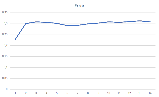
The Expert Advisor was initialized with random weights ranging from -1 to 1, excluding zero values. During testing, already after the 2nd training epoch, the neural network error stabilized around 30%. As you may remember, when learning by the stochastic gradient descent method, the error stabilized around 42% after the 5th training epoch.

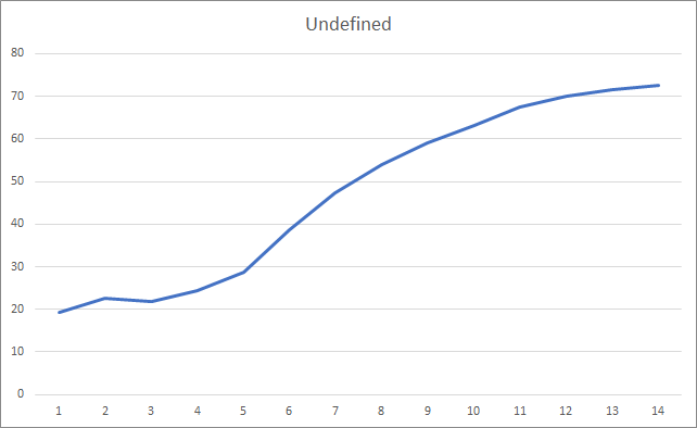
The graph of the missed fractals shows a gradual increase in the value throughout the entire training. However, after 12 training epochs, there is a gradual decrease in the value growth rate. The value was equal to 72.5% after the 14th epoch. When training a similar neural network using the stochastic gradient descent method, the percentage of missing fractals after 10 epochs was 97-100% with different learning rates.

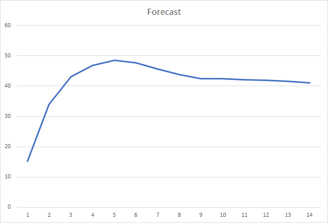
And, probably, the most important metric is the percentage of correctly defined fractals. After the 5th learning epoch, the value reached 48.6% and then gradually decreased to 41.1%. When using the stochastic gradient descent method, the value did not exceed 10% after 90 epochs.

Conclusions

The article considered adaptive methods for optimizing neural network parameters. We have added the Adam optimization method to the previously created neural network model. During testing, the neural network was trained using the Adam method. The results exceed those received previously, when training a similar neural network using the stochastic gradient descent method.

The work done shows our progress towards the goal.

References

1. Neural networks made easy
2. Neural networks made easy (Part 2): Network training and testing
3. Neural networks made easy (Part 3): Convolutional networks
4. Neural networks made easy (Part 4): Recurrent networks
5. Neural networks made easy (Part 5): Multithreaded calculations in OpenCL
6. Neural networks made easy (Part 6): Experimenting with the neural network learning rate
7. Adam: A Method for Stochastic Optimization

Programs used in the article

#	Name	Type	Description
1	Fractal_OCL_Adam.mq5	Expert Advisor	An EA with the classification neural network (3 neurons in the output layer), using OpenCL and the Adam training method
2	NeuroNet.mqh	Class library	A library of classes for creating a neural network
3	NeuroNet.cl	Code Base	OpenCL program code library