機械学習におけるガウス過程（第2回）：MQL5での分類モデルの実装とテスト

MetaTrader 5 — インディケータ | YYYY年08月DD日, 15:26

はじめに

前回の記事では、ベイズ機械学習モデルであるガウス過程の理論的基礎について学び、MQL5でGPライブラリの作成を開始しました。その中で、GaussianProcessとGPOptimizationObjectiveという2つの主要なクラスについて説明しました。

今回は、主要なインターフェースであるIKernel、ILikelihood、IInferenceの実装を詳しく見て、ライブラリを完成させます。その後、合成データを使用してライブラリをテストし、分類用および回帰用のインジケータを作成します。これらをオンラインモードで動作させ、新しいバーが追加されるたびにモデルを再学習するオンラインモードでの動作を確認します。

IKernelインターフェース

Kernels.mqhファイルにあるIKernelインターフェースは、今回のライブラリで共分散カーネルを実装するための基盤となります。これにより、システムを柔軟かつ容易に拡張できるようになります。つまり、IKernelを利用することで、新しい種類のカーネルや、それらの組み合わせを、コードの基本構造を変更せずに追加できます。

interface IKernel {
    // Calculate the covariance matrix between two data sets
    virtual matrix Compute(const matrix &X1, const matrix &X2) = 0;    
    // Calculate the derivative of the covariance matrix with respect to the given hyperparameter
    // param_index: index of the hyperparameter by which the derivative is taken (starting from 0)
    virtual matrix ComputeDerivative(int param_index) = 0;   
    // Return the current values of all kernel hyperparameters
    virtual vector GetHyperparameters() const = 0;
    // Set new values for kernel hyperparameters
    virtual void SetHyperparameters(const vector &params) = 0;
    // Return the number of kernel hyperparameters
    virtual int GetNumHyperparameters() const = 0;
    // Return the kernel string name
    virtual string GetName() const = 0;
};

このインターフェースは、あらゆるカーネルの動作の基盤となる最も重要な2つのメソッドを定義します。

Compute(const matrix &X1, const matrix &X2)：2つのデータセット間の共分散行列Kを計算します。
ComputeDerivative(int param_index)：カーネルのハイパーパラメータの1つに対する共分散行列の微分を計算します。param_indexは、微分の対象となるハイパーパラメータのインデックスを指定します。

RBFKernelクラス（放射基底カーネル）

RBFKernelは、Gaussian kernel（ガウスカーネル）またはsquared exponential kernel（二乗指数カーネル）とも呼ばれ、最も一般的に使用される共分散カーネルの1つです。2つのハイパーパラメータによって特徴付けられます。1つは信号分散σ_f（振幅）、もう1つは関数の滑らかさを決定するlength scale（長さ尺度）lです。

//+------------------------------------------------------------------+
//| Kernel RBF class                                                 |
//+------------------------------------------------------------------+
class RBFKernel : public IKernel {
private:
    double length;
    double sigma_f;
    
    int n; // Number of rows in X1;
    int m; // Number of rows in X2;
    
    matrix m_K;     
    matrix m_D_sq; //  matrix of squared distances ||x_i - x_j||^2
            
public:
    //Constructor
    RBFKernel(double ls, double sf) : length(ls), sigma_f(sf) {}
    //Destructor
    ~RBFKernel() {}
        
   matrix Compute(const matrix &X1, const matrix &X2) override {
    n = (int)X1.Rows();
    m = (int)X2.Rows();

   matrix XX(n, m);
   if (!XX.GeMM(X1, X2.Transpose(), 1.0, 0.0))
   {
      Print("Error: Failed to calculate XX = X * X^T");
      return matrix::Zeros(n, m); 
   }

   matrix diag1(n, 1);
   matrix X1_sq = X1 @ X1.Transpose();
   diag1.Col(X1_sq.Diag(), 0);

   matrix diag2(m, 1);
   matrix X2_sq = X2 @ X2.Transpose();
   diag2.Col(X2_sq.Diag(), 0);
       
   m_D_sq = matrix::Ones(n, 1) @ diag2.Transpose() + diag1 @ matrix::Ones(1, m) - 2 * XX;
   m_K = sigma_f * sigma_f * MathExp((-1 * m_D_sq) / (2 * length * length));     
        
   return m_K;
    }
    
     matrix ComputeDerivative(int param_index) override {
        matrix dK(n, m);
      
        switch (param_index) {
            case 0: {               
                dK = (2.0 / sigma_f) * m_K;
                break;
            } 
            case 1: { 
                dK = m_K * (m_D_sq / (length * length * length)); 
                break;
            }            
        }
        return dK;
    }
          
    vector GetHyperparameters() const override {
        vector params(2);
         params[0] = sigma_f;
         params[1] = length;
        return params;
    }
    void SetHyperparameters(const vector &params) override {
        if (params.Size() == 2) {
            sigma_f = params[0];
            length = params[1];
        } 
    }
    int GetNumHyperparameters() const override { return 2; }
    string GetName() const override { return "RBFKernel"; }
};

幸いなことに、RBFカーネルの場合、微分は簡単に求めることができます。

sigma_fに関する微分：

RBFSigma fに関する微分

lに関する微分：

lengthパラメータについては、K行列と(D_sq / length^3)の要素ごとの乗算を行います。ここでD_sqは、ユークリッド距離の二乗を表す行列です。

LinearKernelクラス（線形カーネル）

LinearKernelは、データポイント間に線形関係があると仮定する単純な共分散カーネルです。関数が線形モデルによって近似されると予想される場合や、より複雑な複合カーネルの構成要素として使用される場合によく用いられます。

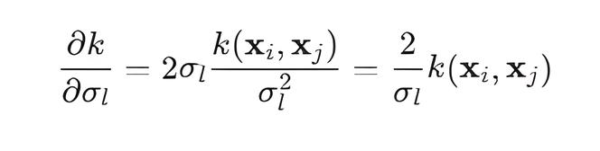
線形カーネルには、信号分散σ_lという1つのハイパーパラメータがあります。

//+------------------------------------------------------------------+
//| Linear kernel class                                              |
//+------------------------------------------------------------------+
class LinearKernel : public IKernel {
private:
    double sigma_l;

    int n; 
    int m; 

    matrix m_K;      
  
public:
     //Constructor
    LinearKernel(double sl): sigma_l(sl){}
     //Destructor
    ~LinearKernel() {}
    
    matrix Compute(const matrix &X1, const matrix &X2) override {
         n = (int)X1.Rows();
         m = (int)X2.Rows();
         m_K.GeMM(X1, X2.Transpose(), sigma_l * sigma_l, 0.0);
        return m_K;
    }
    
    matrix ComputeDerivative(int param_index) override {
        matrix dK(n, m);
        switch (param_index) {
            case 0: { // Derivative with respect to sigma_l         
                dK = (2.0 / sigma_l) * m_K;
                break;
            }           
        }
        return dK;
    }
            
    vector GetHyperparameters() const override {
        vector params(1);       
        params[0] = sigma_l;
        return params;
    }
    void SetHyperparameters(const vector &params) override {
        if (params.Size() == 1) {
            sigma_l = params[0];
        } 
    }
    int GetNumHyperparameters() const override { return 1; }
    string GetName() const override { return "LinearKernel"; }
};

ComputeDerivative(int param_index)メソッド

線形Sigma_Iに関する微分

PeriodicKernelクラス（周期カーネル）

PeriodicKernelは、繰り返しパターンや季節性を持つデータをモデル化するために使用され、周期的な依存関係を捉えることができます。

//+------------------------------------------------------------------+
//| Periodic kernel class                                            |
//+------------------------------------------------------------------+
class PeriodicKernel : public IKernel {
private:
    double sigma_f; //  Signal variance (oscillation amplitude)
    double length;  //  Scale length (smoothness of oscillations)
    double period;  //  Oscillation period
    
    int n; // Number of rows in X1
    int m; // Number of rows in X2
    
    matrix m_K;              // Covariance matrix
    matrix m_D;              // D matrix (sum of derivatives with respect to d  [2 * sin^2(M_PI*distance/period] )
    matrix m_distance_dim[]; // Array of difference matrices for each dimension |x_i_k - x_j_k|
    int    m_d_cols;         // Number of dimensions (features) (X.Cols())
    
public:
    //Constructor
    PeriodicKernel(double ls, double sf, double p) : sigma_f(sf), length(ls), period(p){}  
     //Destructor
    ~PeriodicKernel() {}
  
     matrix Compute(const matrix &X1, const matrix &X2) override {
         n = (int)X1.Rows();
         m = (int)X2.Rows();
        int d = (int)X1.Cols();       
        m_d_cols = d;         
        m_D = matrix::Zeros(n, m); 
        ArrayResize(m_distance_dim, d); 

        for (int k = 0; k < d; k++) {
            vector x1_k = X1.Col(k);
            vector x2_k = X2.Col(k);
    // Create a matrix where each column is a x1_k vector
    // (n x 1) * (1 x m) = (n x m)
    matrix x1_k_copy = x1_k.Outer(vector::Ones(m)) ; 
    // Create a matrix where each row is the transposed vector of x2_k
    // (n x 1) * (1 x m) = (n x m)
    matrix x2_k_copy = vector::Ones(n).Outer(x2_k);
    // Calculate the matrix of all pairwise absolute differences between the elements of vectors x1_k and x2_k
    matrix distance = MathAbs(x1_k_copy - x2_k_copy);
                             
            m_distance_dim[k] = distance; // Cache 'distance' for each dimension (feature)       
            matrix sin_term = MathSin(M_PI * distance / period);
            sin_term = 2.0 * sin_term * sin_term; // 2 * sin^2(u)
            m_D += sin_term; // Sum up element by element
        }        
        // Calculate the K matrix
        m_K = sigma_f * sigma_f * MathExp(-1 * m_D / (length * length));
        return m_K;
    }
       
    matrix ComputeDerivative( int param_index) override {
           matrix dK(n, m);             
        switch (param_index) {
            case 0: { // Derivative with respect to sigma_f
                // dK/d(sigma_f) = (2 / sigma_f) * K               
                dK = (2.0 / sigma_f) * m_K;
                break;
            }
            case 1: { // Derivative with respect to 'length'
                // dK/d(length) = K * (2 * D / length^3)             
                dK = m_K * ( 2.0 * m_D / (length * length * length) ); 
                break;
            }
            case 2: { // Derivative with respect to 'period'
     // dK/d(period) = K * (-1/l^2) * dD/d(period)
    // dD/d(period) = Sum{k=1:d} (2 * pi * (x_ik - x_jk) / period^2) * sin(2*pi*(x_ik - x_jk)/period)
                matrix dD_dp = matrix::Zeros(n, m);
                for (int k = 0; k < m_d_cols; k++) { // Loop through each dimension (column) of the data
                    matrix distance_k = m_distance_dim[k]; // matrix of absolute differences for the k-th dimension              
                    matrix u = M_PI * distance_k / period; // Calculate the argument u_k = pi * |x_ik - x_jk| / period
                    matrix sin_2u = MathSin(2.0 * u); // Calculate sin(2 * u_k) 
                    // Use the already calculated u to calculate //  -pi * |x_ik - x_jk| / period^2  
                    matrix second_term = (-1*u) / period;                          
                   // Accumulate dD/d(period) for the current measurement
                     dD_dp += 2.0 * sin_2u * second_term; 
                }    
                // unite all parts of the derivative
                // dK = K * (-1/length^2) * dD_dp                        
                dK = m_K * (-1.0 / (length * length)) * dD_dp; 
                break;
            }         
        }
        return dK;
    }
    
    vector GetHyperparameters() const override {
        vector params(3);
          params[0] = sigma_f;
          params[1] = length;
          params[2] = period;
        return params;
    }
    void SetHyperparameters(const vector &params) override {
        if (params.Size() == 3) {
            sigma_f = params[0];
            length = params[1];
            period = params[2];
        } 
    }
    int GetNumHyperparameters() const override { return 3; }
    string GetName() const override { return "PeriodicKernel"; }
};

周期カーネルのperiodパラメータに関する微分：

periodパラメータに関する微分の計算は最も難しい部分です。これは、periodが三角関数の内部にあり、その三角関数がさらに指数関数の一部になっているためです。

微分の式は連鎖律に基づいています。ここでは、KがDに依存し、Dが正弦項を介してperiodに依存しています。ComputeDerivativeの実装では、各次元についてdD_dpの成分を順番に計算し、その後、最終的な微分を計算します。

周期カーネルpに関する微分

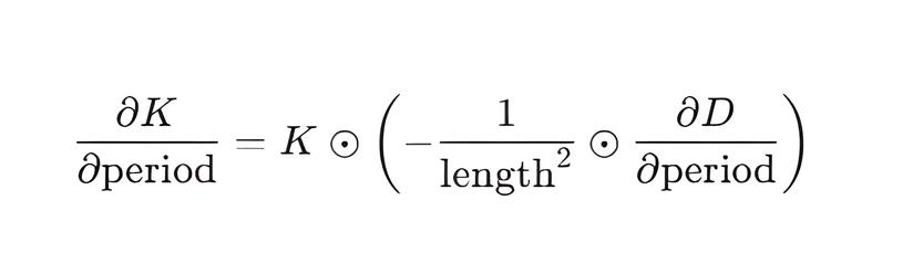
ここでdD_dpは、すべての次元（特徴量）について、2 * sin^2(M_PI * distance / period)の微分を合計することで計算されます。

複合カーネル

ガウス過程では、単純な共分散カーネルを組み合わせることで、データのさまざまな側面（トレンド、周期性、ノイズなど）を表現できる、より複雑なモデルを作成できます。この機能は、次の2つの複合カーネルによって実装されています。

SumKernel：複数のカーネルの共分散行列を加算して組み合わせます。
ProductKernel：複数のカーネルの共分散行列を要素ごとに乗算して組み合わせます。

どちらのクラスも子カーネルのハイパーパラメータを管理し、それらを1つの共有ベクトルにまとめて最適化に使用し、その後、各カーネルへ再配分します。

SumKernelクラス

//+------------------------------------------------------------------+
//| Class for the sum of kernels                                     |
//+------------------------------------------------------------------+
class SumKernel : public IKernel {
private:
    IKernel* kernels[]; 
public:
    // Constructor
    SumKernel(IKernel* &input_kernels[]) {
        ArrayResize(kernels, ArraySize(input_kernels));
        ArrayCopy(kernels, input_kernels);
    }
    //Destructor
    ~SumKernel() {
    for (int i = 0; i < ArraySize(kernels); i++) {
        if (kernels[i] != NULL) {
            delete kernels[i]; 
        }
    }
    ArrayFree(kernels); 
}
    matrix Compute(const matrix &X1, const matrix &X2) override {
        int n = (int)X1.Rows();
        int m = (int)X2.Rows();
        matrix sum = matrix::Zeros(n,m);
        for (int i = 0; i < ArraySize(kernels); i++) {        
                sum += kernels[i].Compute(X1, X2); // Sum the matrices from each child kernel        
        }
        return sum; 
    }
    
    matrix ComputeDerivative(int param_index) override { 
        int current_param_offset = 0; // Start at offset 0 for the first kernel
        for (int i = 0; i < ArraySize(kernels); i++) {
        // Get the number of hyperparameters of the current child kernel
            int num_params_current_kernel = kernels[i].GetNumHyperparameters();
                
    //  Check if the global param_index belongs to the current child kernel
    //   param_index should be:
    //   - greater than or equal to the current offset
    //   - strictly less than the current offset + the number of parameters of the current kernel 
                if (param_index >= current_param_offset && 
                    param_index < current_param_offset + num_params_current_kernel) {                   
     //  If param_index belongs to this kernel, calculate its local index
                    int local_param_index = param_index - current_param_offset;                   
        //    Call ComputeDerivative on the found child kernel and
        //    pass it the local index.
        //    Since the derivative of the sum of kernels with respect to the parameter of one kernel is equal to the derivative
        //    of this particular kernel by this parameter, we can immediately return the result
                    return kernels[i].ComputeDerivative(local_param_index);
                }               
    //    If param_index does not belong to the current kernel,
    //    increase the offset to check the next kernel
                current_param_offset += num_params_current_kernel;           
        }  
     Print("Error: SumKernel::ComputeDerivative - Parameter index ", param_index, " out of bounds");
        return matrix::Zeros(1, 1);     
    }    
 
//+---------------------------------------------------------------------------------+
//| The function returns the values of all hyperparameters of the composite kernel  |
//+---------------------------------------------------------------------------------+  
   vector GetHyperparameters() const override {
        vector all_params(GetNumHyperparameters()); 
        int current_idx = 0;
        for (int i = 0; i < ArraySize(kernels); i++) {
        // Get the values of the parameters of the current child kernel
           vector kernel_params = kernels[i].GetHyperparameters(); 
                for (int j = 0; j < (int)kernel_params.Size(); j++) {
                 // Copy the parameters into the common vector
                    all_params[current_idx + j] = kernel_params[j];
                }
                // Update the offset for the next kernel
                current_idx += (int)kernel_params.Size();
        }
        return all_params;
    }
//+----------------------------------------------------------------------+
//|The function takes a vector of values of all hyperparameters, breaks  |
//|it into the appropriate parts and assigns them to each child kernel   |
//+----------------------------------------------------------------------+  
    void SetHyperparameters(const vector &params) override {
        int current_idx = 0;
        for (int i = 0; i < ArraySize(kernels); i++) {
               // Get the number of hyperparameters of the current child kernel
                int num_params = kernels[i].GetNumHyperparameters();
                vector sub_params(num_params); 
                // Copy the corresponding parameters from the general vector
                for (int j = 0; j < num_params; j++) {
                    sub_params[j] = params[current_idx + j];
                }
         // Call the SetHyperparameters() method on the current child kernel,
        // passing it only its own parameters, collected in the sub_params vector
                kernels[i].SetHyperparameters(sub_params);
                current_idx += num_params;
        }
    }
//+--------------------------------------------------------------------------------------+
//| Return the total number of hyperparameters for the entire SumKernel composite kernel |                                                                 
//+--------------------------------------------------------------------------------------+  
    int GetNumHyperparameters() const override {
        int total_params = 0;
        for (int i = 0; i < ArraySize(kernels); i++) {
                total_params += kernels[i].GetNumHyperparameters(); 
        }
        return total_params;
    }
    
    string GetName() const override {
        string name = "Sum(";
        for (int i = 0; i < ArraySize(kernels); i++) {
                name += kernels[i].GetName();
                if (i < ArraySize(kernels) - 1) name += ",";
        }
        name += ")";
        return name;
    }
 //+------------------------------------------------------------------+
 //| Provide external access to the list of child kernels             |
 //+------------------------------------------------------------------+   
    void GetKernels(IKernel* &output_kernels[]) const {
    // Copy pointers from the internal kernels array to the passed 
    // output_kernels external array. This provides access to child
    // kernels in the GaussianProcess::Fit() method, where it is necessary to iterate through
    // all elementary kernels to set optimization boundaries
    // of their hyperparameters.
        ArrayCopy(output_kernels, kernels);
    }
};

Computeメソッドは、各子カーネルから返される共分散行列を単純に加算し、最終的な共分散行列Kを計算します。ここではポリモーフィズムの原則が機能しています。kernels配列にはIKernel*という基底型のポインタが格納されていますが、kernels[i].Compute(X1, X2)を呼び出すと、実際にはそれぞれの子カーネル固有のCompute実装が呼び出されます。これにより、SumKernelはIKernelを継承したあらゆるカーネルを扱うことができます。

ComputeDerivativeメソッドの重要な考え方は、カーネルの和の共分散関数について、特定のハイパーパラメータに関する微分は、そのハイパーパラメータが属する子カーネルの共分散関数の微分に等しいということです。つまり、ComputeDerivativeはparam_indexによって対応する子カーネルを見つけ、そのカーネルからの微分のみを返します。その他の子カーネルのパラメータに関する微分はゼロとみなされます。

ProductKernelクラス

//+------------------------------------------------------------------+
//| Class for the product of kernels                                 |
//+------------------------------------------------------------------+
class ProductKernel : public IKernel {
private:
    IKernel* kernels[];
    
    matrix m_X1;
    matrix m_X2;
    int n; 
    int m; 
    
public:
   // Constructor: copies pointers to child kernels
    ProductKernel(IKernel* &input_kernels[]) {
        ArrayResize(kernels, ArraySize(input_kernels));
        ArrayCopy(kernels, input_kernels);
    }
   // Destructor 
    ~ProductKernel()
    {
        for (int i = 0; i < ArraySize(kernels); i++) {
            if (kernels[i] != NULL){ delete kernels[i]; }
        }
        ArrayFree(kernels); 
    }
    matrix Compute(const matrix &X1, const matrix &X2) override {
         n = (int)X1.Rows();
         m = (int)X2.Rows();
         m_X1 = X1;
         m_X2 = X2;
        
        matrix product = matrix:: Ones(n,m);
        for (int i = 0; i < ArraySize(kernels); i++) {
        // Polymorphism: call the Compute() method of each child kernel,
        // regardless of its specific type, and multiply the result element by element
                product *= kernels[i].Compute(X1, X2);
        }
        return product;
    }
    
    matrix ComputeDerivative(int param_index) override {    
        matrix dK_prod(n, m); // Final derivative matrix      
        int current_param_offset = 0;
        int target_kernel_idx = -1; // Kernel index the hyperparameter belongs to
        int local_param_index = -1; // Local index of the hyperparameter in this kernel

        // Step 1: Find the kernel and local index of the hyperparameter
        for (int i = 0; i < ArraySize(kernels); i++) {
                int num_params_current_kernel = kernels[i].GetNumHyperparameters();
                
                if (param_index >= current_param_offset && 
                    param_index < current_param_offset + num_params_current_kernel) {
                    
                    target_kernel_idx = i;
                    local_param_index = param_index - current_param_offset;
                    break; 
                }
                
                current_param_offset += num_params_current_kernel;
        }

        if (target_kernel_idx == -1) {
            Print("Error: ProductKernel::ComputeDerivative - Parameter index ", param_index, " out of bounds");
            return matrix::Zeros(1, 1);
        }
        
        // Step 2: Calculate dK_k / d_theta_j for the target kernel
        matrix dK_target_kernel = kernels[target_kernel_idx].ComputeDerivative(local_param_index);
        
        // Step 3: Calculate the K_m product for all other kernels (m != k)
        matrix other_kernels_product = matrix::Ones(n, m); 
        for (int i = 0; i < ArraySize(kernels); i++) {
            if (i != target_kernel_idx) { //  Skip the target kernel
                other_kernels_product = other_kernels_product * kernels[i].Compute(m_X1, m_X2); 
            }
        }
        // Step 4: Multiply the results element by element
        dK_prod =  dK_target_kernel * other_kernels_product; 
        return dK_prod;
    }   
     
 // Collect the hyperparameter values of all child kernels into a single vector   
 vector GetHyperparameters() const override {
        vector all_params(GetNumHyperparameters()); 
        int current_idx = 0;
        for (int i = 0; i < ArraySize(kernels); i++) {
                vector kernel_params = kernels[i].GetHyperparameters();
                for (int j = 0; j < (int)kernel_params.Size(); j++) {
                    all_params[current_idx + j] = kernel_params[j];
                }
                current_idx += (int)kernel_params.Size();
        }
        return all_params;
    }
        
    void SetHyperparameters(const vector &params) override {
        int current_idx = 0;
        for (int i = 0; i < ArraySize(kernels); i++) {
                int num_params_kernel = kernels[i].GetNumHyperparameters();
               vector sub_params(num_params_kernel); 
                for (int j = 0; j < num_params_kernel; j++) {
                    sub_params[j] = params[current_idx + j];
                }
                kernels[i].SetHyperparameters(sub_params);
                current_idx += num_params_kernel;
        }
    }
    int GetNumHyperparameters() const override {
        int total_params = 0;
        for (int i = 0; i < ArraySize(kernels); i++) {
                total_params += kernels[i].GetNumHyperparameters();
        }
        return total_params;
    }
    string GetName() const override {
        string name = "Prod(";
        for (int i = 0; i < ArraySize(kernels); i++) {
                name += kernels[i].GetName();
                if (i < ArraySize(kernels) - 1) name += "*";
        }
        name += ")";
        return name;
    }
 //+------------------------------------------------------------------+
 //| Provide external access to the list of child kernels             |
 //+------------------------------------------------------------------+   
    void GetKernels(IKernel* &output_kernels[]) const {
        ArrayCopy(output_kernels, kernels);
    }
};

Computeメソッドは、各子カーネルから返される共分散行列を要素ごとに乗算し、最終的な共分散行列Kを計算します。SumKernelと同様に、ポリモーフィズムを使用して、対応する子カーネルのComputeメソッドを呼び出します。
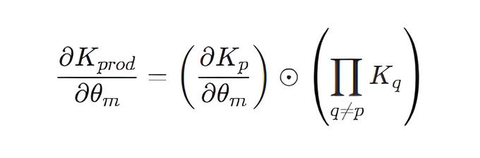
ComputeDerivativeメソッド：特定のK_p子カーネルに属するハイパーパラメータに関するKの微分を計算するために、ProductKernelではライプニッツの積の微分法則を適用します。あるパラメータに関するKの微分は、そのパラメータに関するK_p行列の微分と、その他すべての子カーネルの共分散行列を微分せずに要素ごとに乗算したものの積に等しくなります。

積カーネルに関する微分

ILikelihoodインターフェース

ILikelihoodインターフェースは、ライブラリ内のあらゆる尤度関数がどのように動作するべきかを定義します。これにより、連続値（回帰の場合）や離散的なカテゴリー（分類の場合）など、さまざまなタイプのデータを扱うことができます。

//+------------------------------------------------------------------+
//|Interface for likelihood functions                                |
//+------------------------------------------------------------------+
interface ILikelihood {
    // Compute the p(y|f) log-likelihood for latent values f and observed values y
    virtual double LogLikelihood(const vector &f, const vector &y) = 0;
    //----------------------------- Derivatives of the logarithm of the likelihood with respect to f ----------------- 
    // Calculate the vector of the first derivative of the log-likelihood with respect to f (dlp/df)
    virtual vector LogLikelihoodGradient(const vector &f, const vector &y) = 0;   
    // Compute the second derivative (Hessian) matrix of the log-likelihood with respect to f (d^2lp/df df^T)
    virtual matrix LogLikelihoodHessian(const vector &f, const vector &y) = 0;   
    // Calculate the vector of the third derivative of the log-likelihood with respect to f (d^3lp/df^3)
    virtual vector LogLikelihoodThirdDerivative(const vector &f, const vector &y) = 0; 
    //----------------------------- Derivatives of the logarithm of the likelihood with respect to the parameters -----------------  
    // The first derivative of the log-likelihood with respect to the j-th likelihood hyperparameter.
    virtual double LogLikelihoodGradientParam(const vector &f, const vector &y, int param_index) = 0;   
    // Hessian derivative of the log-likelihood with respect to the j-th likelihood hyperparameter.
    virtual matrix LogLikelihoodHessianDerivative(const vector &f, const vector &y, int param_index) = 0;
    
    // Return the name of the likelihood function
    virtual string GetName() const = 0;
    // Return the current values of the likelihood hyperparameters 
    virtual vector GetHyperparameters() const = 0;
    // Set new values for the likelihood hyperparameters
    virtual void SetHyperparameters(const vector &params) = 0;
    // Return the number of likelihood hyperparameters
    virtual int GetNumHyperparameters() const = 0;
};

GaussianLikelihoodクラス

GaussianLikelihoodは、観測データに正規ノイズが存在することを前提とした回帰問題に対する尤度関数を実装しています。

//+------------------------------------------------------------------+
//| Gaussian likelihood class (for regression problems)              |
//+------------------------------------------------------------------+
class GaussianLikelihood : public ILikelihood {
private:
    double m_noise_sigma; // Noise parameter (standard deviation) 
public:
    // Constructor 
    GaussianLikelihood(double initial_noise_sigma) : m_noise_sigma(initial_noise_sigma) {}
    
    // Return the current value of the hyperparameter 
    vector GetHyperparameters() const override {
        vector params(1);
        params[0] = m_noise_sigma;
        return params;
    }
    // Set a new hyperparameter value
    void SetHyperparameters(const vector &params) override {
        if (params.Size() == 1) {
            m_noise_sigma = params[0];
        } 
    }
     // Return the number of hyperparameters 
    int GetNumHyperparameters() const override { return 1; }
    
    // Calculate the log p(y|f) log-likelihood for a Gaussian distribution
    double LogLikelihood(const vector &f, const vector &y) override {
        int n = (int)y.Size();
        double noise_variance = m_noise_sigma * m_noise_sigma;       
        vector residual = y - f;
        // Formula for the logarithm of the density of a multivariate normal distribution      
        return -0.5 / noise_variance * (residual @ residual) - 0.5 * n * MathLog(2 * M_PI * noise_variance);
    }
    
   //------------------ Derivatives with respect to f -----------------------
   // Calculate the vector of the first derivative of the log-likelihood with respect to f (dlp/df)
    vector LogLikelihoodGradient(const vector &f, const vector &y) override {
        // d(log p(y|f))/df = (y - f) / sigma^2
        return (y - f) / (m_noise_sigma * m_noise_sigma);
    }
   // Compute the second derivative (Hessian) matrix of the log-likelihood with respect to f (d^2lp/dfdf^T) 
    matrix LogLikelihoodHessian(const vector &f, const vector &y) override {
        // d^2(log p(y|f))/dfdf^T = -1/sigma^2 * I
        int n = (int)y.Size();
        return matrix::Identity(n, n) * (-1.0 / (m_noise_sigma * m_noise_sigma));
    }   
    // Calculate the vector of the third derivative of the log-likelihood with respect to f
    vector LogLikelihoodThirdDerivative(const vector &f, const vector &y) override {
        // For Gaussian likelihood d^3(log p(y|f))/df^3 = 0
        return vector::Zeros((int)y.Size()); 
    }
   
   // ------------------------------ Derivatives with respect to the parameter -----------------------------------    
   // // Calculate the first derivative of the log-likelihood with respect to the j-th likelihood hyperparameter
    virtual double LogLikelihoodGradientParam(const vector &f, const vector &y, int param_index) override {
        // Gaussian likelihood has only 1 hyperparameter: m_noise_sigma (index 0)
        if (param_index == 0) {
            // Formula for d(log p(y|f))/d(sigma_n):
            // = (y-f)^T(y-f) / sigma_n^3 - N / sigma_n
            vector y_minus_f = y - f;
            double sn3 = m_noise_sigma * m_noise_sigma * m_noise_sigma;            
            double term1 = (y_minus_f @ y_minus_f) / sn3;
            double term2 = y.Size() / m_noise_sigma; // N / sigma_n
            return term1 - term2;

        } else {
           return 0.0; 
        }
    }
    
    // Calculate the Hessian derivative of the log-likelihood with respect to the j-th likelihood hyperparameter
    matrix LogLikelihoodHessianDerivative(const vector &f, const vector &y, int param_index) override {
        int n = (int)y.Size();
        if (param_index == 0) {
            // Derivative of Hessian with respect to m_noise_sigma: d/d(sigma_n) [-1/sigma_n^2 * I] = (2/sigma_n^3) * I
            double derivative_coeff = 2.0 / (m_noise_sigma * m_noise_sigma * m_noise_sigma);
            return matrix::Identity(n, n) * derivative_coeff;
        } else {
            return matrix::Zeros(n, n); 
        }
    }
            
    string GetName() const override { return "GaussianLikelihood"; }
};

主なメソッドは以下のとおりです。

GaussianLikelihoodコンストラクタ：1つのハイパーパラメータであるノイズの標準偏差を初期化します。
LogLikelihood()：多変量正規分布の確率密度関数に対するp(y∣f)の対数尤度を計算します。

Gauss loglike

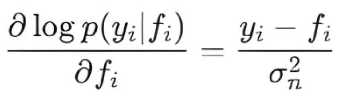
LogLikelihoodGradient()：潜在値fに関する対数尤度の1階微分を計算します。これはベクトルであり、各要素は次の値に等しくなります。

Gradient Gauss loglike

LogLikelihoodHessian()：fに関する対数尤度の2階微分（ヘッセ行列）を計算します。ガウス尤度の場合、ヘッセ行列は対角行列になります。

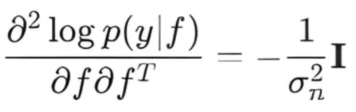
LogLikelihoodThirdDerivative()：3階微分を計算します。ガウス尤度の場合、2階を超えるすべての微分はゼロになります。
LogLikelihoodGradientParam()：m_noise_sigmaハイパーパラメータに関する対数尤度の1階微分を計算します。

Gradient param Gauss loglike

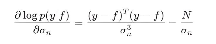
LogLikelihoodHessianDerivative()：m_noise_sigmaハイパーパラメータに関する対数尤度のヘッセ行列の微分を計算します。

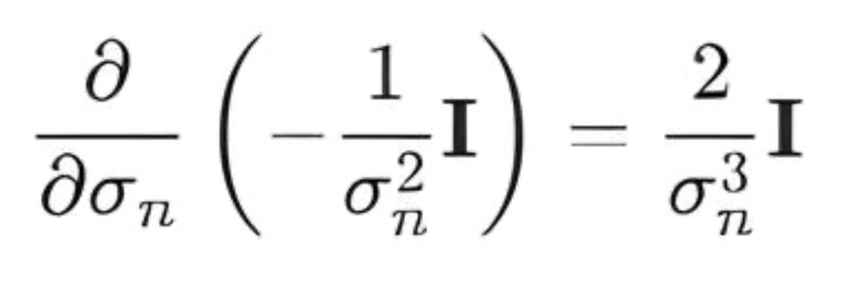
Hessian Derivative param Gauss loglike

LogitLikelihoodクラス

LogitLikelihoodは、観測された目的変数yが{−1,+1}の値を取る二値分類に使用されます。潜在関数fとクラス所属確率を、シグモイド関数を介して関連付けます。

LogitLikelihoodの実装では、大きな入力値や小さな入力値に対するチェックを備えたsigmoid()およびSoftplus()補助関数を提供します。

//+------------------------------------------------------------------+
//| Class for Logit likelihood (y {-1, +1})                          |
//+------------------------------------------------------------------+
class LogitLikelihood : public ILikelihood {
public:
    // logit_sigmoid(x) = 1 / (1 + exp(-x))
    double sigmoid(double x) const {
        if (x > 100.0) return 1.0;     // Avoid NaN occurrences
        if (x < -100.0) return 0.0;    
        return 1.0 / (1.0 + MathExp(-x));
    }

    // Softplus log(1 + exp(x)) function
    double Softplus(double x) const {
        if (x > 100.0) return x;           // For very large x, log(1 + exp(x)) ~ x
        if (x < -100.0) return MathExp(x); // For very small x, log(1 + exp(x)) ~ exp(x)
        return MathLog(1.0 + MathExp(x));
    }

public:
    // Constructor (logit likelihood has no hyperparameters of its own) 
    LogitLikelihood() {}
   
    vector GetHyperparameters() const override {
        return vector::Zeros(0); 
    }
   
    void SetHyperparameters(const vector &params) override {}   
    // Return the number of likelihood hyperparameters 
    int GetNumHyperparameters() const override { return 0; }
    
    // --- Calculate the log-likelihood: log p(y|f) ---
    // Formula: sum_i (-log(1 + exp(-y_i * f_i)))
    double LogLikelihood(const vector &f, const vector &y) override {
        int n = (int)y.Size();
        double total_log_likelihood = 0.0;       
        for (int i = 0; i < n; i++) {
            total_log_likelihood += -Softplus(-y[i] * f[i]);
        }
        return total_log_likelihood;
    }
    
   //  Compute the gradient of the log-likelihood with respect to f
  //   Formula: d(log p(y_i|f_i))/df_i = y_i * sigma(-y_i * f_i)
    vector LogLikelihoodGradient(const vector &f, const vector &y) override {
        int n = (int)y.Size();
        vector grad(n);
        for (int i = 0; i < n; i++) {
            grad[i] = y[i] * sigmoid(-y[i] * f[i]);
         // grad[i] = y[i] * (1 - sigmoid(y[i] * f[i])); equivalent to
        }
        return grad;
    }
       
    // Compute the Hessian of the log-likelihood of f (the H diagonal matrix)
    // Formula: d^2(log p(y_i|f_i))/df_i^2 = -sigma(y_i*f_i)(1 - sigma(y_i*f_i))
    matrix LogLikelihoodHessian(const vector &f, const vector &y) override {
        int n = (int)y.Size();
        matrix H = matrix::Identity(n, n); 
        for (int i = 0; i < n; i++) {
            double sig = sigmoid(y[i] * f[i]);
            H[i][i] = -1*sig * (1.0 - sig); 
        }
        return H;
    }
    
    // Calculate the third derivative of the log-likelihood with respect to f
    // Formula: d^3(log p(y_i|f_i))/df_i^3 = y_i * sigma(-y_i f_i) * (1 - sigma(-y_i f_i)) * (1 - 2*sigma(-y_i f_i))
    vector LogLikelihoodThirdDerivative(const vector &f, const vector &y) override {
        int n = (int)y.Size();
        vector third_deriv(n);
        for (int i = 0; i < n; i++) {           
            double sig_neg_yf = sigmoid(-y[i] * f[i]);         
            third_deriv[i] = y[i] * sig_neg_yf * (1.0 - sig_neg_yf) * (1.0 - 2.0 * sig_neg_yf);          
            // equivalent to
           //  double sig_yf = sigmoid(y[i] * f[i]);         
           // third_deriv[i] = -y[i] * sig_yf * (1.0 - sig_yf) * (1.0 - 2.0 * sig_yf);
        }
        return third_deriv;
    }
        
    // LogitLikelihood has no hyperparameters
    virtual double LogLikelihoodGradientParam(const vector &f, const vector &y, int param_index) override {        
        return 0.0;
    }      
    // LogitLikelihood has no hyperparameters
    matrix LogLikelihoodHessianDerivative(const vector &f_latent, const vector &y, int param_index) override {
        int n = (int)y.Size();
        return matrix::Zeros(n, n); 
    }
   
    string GetName() const override { return "LogitLikelihood"; }
};

主なメソッドは以下のとおりです。

LogLikelihood()：対数尤度logp(y∣f)を計算します。y ∈ {−1,+1}の二値分類の場合、これは二値クロスエントロピー尤度の対数の合計になります。

Logit loglike

LogLikelihoodGradient()：fに関する対数尤度の1階微分を計算します。勾配ベクトルの各要素は次の値に等しくなります。

Gradient Logit loglike

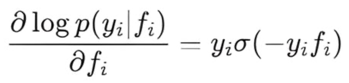
LogLikelihoodHessian()：fに関する対数尤度の2階微分（ヘッセ行列）を計算します。ロジット尤度の場合、ヘッセ行列は対角行列であり、その対角要素は次の値に等しくなります：

Hessian Logit loglike

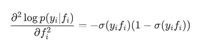
LogLikelihoodThirdDerivative()：fに関する対数尤度の3階微分を計算します。ベクトルの各要素は次の値に等しくなります。

Third Derivative Logit loglike

補助関数と構造体

StructUtils.mqhファイルには、GPを扱いやすくするための列挙型、データ構造、関数がまとめられています。

    enum PredictMode {
    PROBIT      = 0,  // Probit Approximation
    NUM_INTEGR  = 1,  // Numerical integration
    MONTE_CARLO = 2   // Monte Carlo
    
};

//--- Structure for prediction results 
struct GPPredictionResult
{
    vector mu_f_star;    // Posterior mean for the latent f* function on new data   
    matrix Sigma_f_star; // Posterior covariance for the latent f* function on new data
    
    // Regression-only fields (GaussianLikelihood)
    vector mu_y_star;      // Posterior mean of observations y*
    matrix Sigma_y_star;   // Posterior covariance of observations y*
    
    // Fields for classification only (LogitLikelihood, ProbitLikelihood, etc.)
    vector predicted_probabilities; // Probabilities p(y*=+1 | X*, D) 
    vector predicted_labels;        // Predicted y* labels (+1 or -1)
};

// Structure for the inference result
struct GPInferenceResult {
    double      nlml_value;    // Negative logarithm of the marginal likelihood
    vector      nlml_gradient; // NLML gradient by kernel and likelihood hyperparameters
    
    // Inference results on training data:
    vector      mu_f_train;    // Posterior mean of the latent function f on the training data
    matrix      Sigma_f_train; // Posterior covariance of the latent function f on the training data (K^−1+W)^−1 
    matrix      L_K_noisy;     // Cholesky decomposition K_noisy = cholesky(K + s2n*I)
    matrix      L_B;           // Cholesky decomposition B = I + W^0.5 @ K @ W^0.5
    matrix      sW;            // sW = W^0.5;
    vector      sW_diag;       // sW diagonal
    matrix      sW_K;          // sW @ K
    vector      alpha;         // (K_noisy)^-1 * y 
    matrix      H;             // Hessian of the log likelihood d^2 log p(y|f)/df^2 (for LaplaceInference)    
    bool        success;       // Flag indicating success of the inference function
};

PredictMode列挙型は、分類モデルで予測を実行するためのさまざまなモードを定義します。
GPInferenceResult構造体は、推論中に得られたすべての主要な結果を保存するために使用されます。
GPPredictionResult構造体は、新しい（テスト）データX_testに対して予測を実行した後に得られるすべての結果を保存するために設計されています。

これらのユーティリティは、推論メソッドを効率的に実装するために必要であり、モデル内の計算を大幅に高速化します。

DiagonalTrace

//+-------------------------------------------------------------------+
//| Compute the trace of the product of two matrices using only       |
//| diagonal elements of the final matrix                             |
//+-------------------------------------------------------------------+
double DiagonalTrace(const matrix &A, const matrix &B)
  {
   ulong m = A.Rows();
   ulong n = A.Cols();
   ulong n_b = B.Rows();
   ulong p = B.Cols();
// Find the minimum size for the diagonal
   ulong k = MathMin(m, p);
   double tr = 0.0;

   for(ulong i = 0; i < k; i++)
     {
      // Dot product of the i-th row of A and the i-th column of B
      tr += A.Row(i)@B.Col(i);
     }
   return tr;
  }

AとBという2つの行列の積のトレースTr(A @ B)を、行列全体の積を作成することなく計算します。これは、行列Aの各行と、行列Bの対応する列とのスカラー積を合計することでおこないます。これにより、行列全体を乗算する場合と比較して、計算コストを大幅に削減できます。

cho_solve（OpenBLAS LinearEquationsSolutionTriangularラッパー）

 //+-----------------------------------------------------------------------+
   //| Solve the system A*X = B using the Cholesky decomposition A = LL^T  |
   //| Parameters:                                                         |
   //|   c: Lower triangular matrix L from the Cholesky decomposition      |
   //|   b: right side of the system (matrix)                              |
   //| Return: matrix X - system solution                                  |
   //+---------------------------------------------------------------------+
   matrix            cho_solve(const matrix &c, const matrix &b)
     {
    // Check if 'c' matrix is lower triangular one
    if (!c.IsLowerTriangular()) {
        Print("Error: cho_solve - Input matrix 'c' is not lower triangular.");
        return matrix::Zeros(c.Rows(), b.Cols());
    }

// Step 1: Solve L * Y = B 
    //  Y -  intermediate matrix, the result of solving L^-1 * B
    matrix Y;
    if (!c.LinearEquationsSolutionTriangular(EQUATIONSFORM_N, b, Y)) {
        PrintFormat("Error: cho_solve- LinearEquationsSolutionTriangular L * Y = B failed. Error Code: %d", GetLastError());
        return matrix::Zeros(c.Rows(), b.Cols());
    }

// Step 2: Solve L^T * X = Y 
    //  X - L^T * X = Y system solution, which is equivalent to (L^T)^-1 * Y
    matrix X;
    if (!c.LinearEquationsSolutionTriangular(EQUATIONSFORM_T, Y, X)) {
        PrintFormat("Error: cho_solve- LinearEquationsSolutionTriangular L^T * X = Y failed. Error Code: %d", GetLastError());
        return matrix::Zeros(c.Rows(), b.Cols());
        }
      return X;
     }

   //+------------------------------------------------------------------+
   //| Solve the system Ax = b using the Cholesky decomposition A = LL^T|
   //| Parameters:                                                      |
   //|   c: Lower triangular matrix L from the Cholesky decomposition   |
   //|   b: right side of the system (vector)                           |
   //| Return: vector x - system solution                               |
   //+------------------------------------------------------------------+
   vector            cho_solve(const matrix &c, const vector &b)
     {
      // Check if 'c' matrix is lower triangular one
    if (!c.IsLowerTriangular()) {
        Print("Error: cho_solve - Input matrix 'c' is not lower triangular");
        return vector::Zeros(c.Rows()); 
    }

    // Step 1: Solve L * y = b 
    // y - intermediate vector, the result of solving L^-1 * b
    vector y;
    if (!c.LinearEquationsSolutionTriangular(EQUATIONSFORM_N, b, y)) {
        PrintFormat("Error: cho_solve- LinearEquationsSolutionTriangular L * y = b failed. Error Code: %d", GetLastError());
        return vector::Zeros(c.Rows());
    }

    // Step 2: Solve L^T * x = y
    // x - final solution of the L^T * x = y system, which is equivalent to (L^T)^-1 * y
    vector x;
    if (!c.LinearEquationsSolutionTriangular(EQUATIONSFORM_T, y, x)) {
        PrintFormat("Error: cho_solve- LinearEquationsSolutionTriangular L^T * x = y failed. Error Code: %d", GetLastError());
        return vector::Zeros(c.Rows());
    }
      return x;
     }

cho_solve関数は、行列Aがコレスキー分解A = LL^Tによって得られる場合に、連立一次方程式Ax = b（または行列Bに対するAX = B）を効率的に解くために設計されています。ここでLは下三角行列です。

A.Inv()によってA^−1を直接計算する方法は、リソースを多く消費し、数値的に不安定になる可能性があります。一方、コレスキー分解は、より効率的で堅牢な方法を提供します。

cho_solve内部では、内部では、主に2つの処理がおこなわれます。

前進代入：LY = B（またはLy = b）という連立方程式を解きます。ここでLは入力行列c、Y（またはy）は中間結果です。Lは三角行列であるため、この計算は比較的高速です。

後退代入：続いて、L^TX = Y（またはL^Tx = y）という連立方程式を解きます。ここでL^TはLの転置行列です。L^Tは上三角行列であるため、この計算も効率的に実行できます。

これらの処理は、高性能な線形代数ライブラリであるOpenBLASのLinearEquationsSolutionTriangular関数を使用して実装されています。これにより計算速度を大幅に向上させることができ、ガウス過程のような計算負荷の高い機械学習モデルにおいて不可欠な機能となります。

IInferenceインターフェース

interface IInference
  {
// This method performs inference (i.e., computes the posterior distribution of f)
// and returns the components needed for NLML and prediction
   virtual void Infer(const matrix &X, const vector &y,
                      IKernel *kernel, ILikelihood *likelihood,GPInferenceResult &result) = 0;
   virtual string GetName() const = 0;
  };

このインターフェースにより、GaussianProcessのコアロジックを変更することなく、ガウス尤度に対する厳密推論や、ガウス以外の場合の近似手法など、異なる推論手法を切り替えることができます。

Inferメソッドは、このインターフェースの中心となります。このメソッドは、潜在関数fの事後分布に対する推論を実行し、その後の計算（NLMLおよび予測）に必要な各要素を返します。以下の引数を受け取ります。

X：学習用特徴量の行列
y：学習用ラベルのベクトル
kernel：IKernelオブジェクトへのポインタ
likelihood：ILikelihoodオブジェクトへのポインタ
result：すべての推論結果を格納するために使用されるGPInferenceResult構造体への参照。以下を含みます。

周辺尤度の負の対数(NLML)：ハイパーパラメータの最適化に必要です。
NLML勾配のベクトル：すべてのカーネルおよび尤度ハイパーパラメータに対するNLMLの勾配です。
補助行列およびベクトル：L_K_noisy、L_B、sW、mu_f_train、Sigma_f_train、alpha。これらは、NLMLの勾配計算およびその後の新しいデータの予測に使用されます。

ExactInferenceクラス

//+------------------------------------------------------------------+
//| ExactInference For Gaussian likelihood only                      |
//+------------------------------------------------------------------+
class ExactInference : public IInference
  {

public:
                     ExactInference() {}

   void              Infer(const matrix &X, const vector &y,
                           IKernel *kernel, ILikelihood *likelihood,GPInferenceResult &result) override
     {
      if(likelihood.GetName() != "GaussianLikelihood")
        {
         Print("ExactInference supports only GaussianLikelihood");
         result.nlml_value = DBL_MAX;
         return;
        }
      result.success = false;
      int n = (int)y.Size();

      //  Calculate K with current kernel parameters
      matrix K = kernel.Compute(X, X);

      //  Get the noise variance
      vector likelihood_params = likelihood.GetHyperparameters();
      double sigma = likelihood_params[0];
      double variance = sigma * sigma;

      double jitter = 1e-6;
      matrix K_noisy = K + matrix::Identity(n, n) * (variance + jitter);

      if(!K_noisy.Cholesky(result.L_K_noisy))
        {
         PrintFormat("Error: Cholesky decomposition failed. Error Code: %d",GetLastError());
         result.nlml_value = DBL_MAX;
         return;
        }
      //------------- Algorithm 2.1 GPML ---------------------------
      //Calculate alpha (K_noisy^-1 * y) - O(N^2)
      result.alpha = cho_solve(result.L_K_noisy, y);
      //+------------------------------------------------------------------+
      //| NLML = 0.5y^T(K+σ^2*I)^-1*y + 0.5*log|K+σ^2*I| +n/2*Log(2π)      |
      //+------------------------------------------------------------------+
      //+------------------------------------------------------------------+
      //| NLML = 0.5y^T*alpha         + 0.5*log|K+σ^2*I| +n/2*Log(2π)      |
      //+------------------------------------------------------------------+
      // --- Calculate the first term in the NLML equation:
      double data_term = 0.5 * (y @ result.alpha);
      // --- Calculate the second term: 1/2 * log|K + sigma^2*I| = sum(log(L_ii))
      double log_det = MathLog(result.L_K_noisy.Diag()).Sum();
      // --- Calculate the third term: n/2 * log(2π)
      double const_term = 0.5 * n * MathLog(2 * M_PI);
      //--- NLML
      result.nlml_value = data_term + log_det + const_term;

      // -------------------- NLML gradients calculations --------------------------------------
      result.nlml_gradient.Resize(kernel.GetNumHyperparameters() + likelihood.GetNumHyperparameters());
      int current_grad_idx = 0;
      // Calculate (K_noisy^-1)
      matrix K_noisy_inv = cho_solve(result.L_K_noisy, matrix::Identity(n, n));

      // 1. Gradients on kernel hyperparameters
      vector kernel_hyperparams = kernel.GetHyperparameters();
      // Calculate aatK_noisy_inv once before the loop - O(N^2)
      matrix aatK_noisy_inv = result.alpha.Outer(result.alpha) - K_noisy_inv;
      matrix dK_dtheta;
      for(int i = 0; i < (int)kernel_hyperparams.Size(); i++)
        {
         dK_dtheta = kernel.ComputeDerivative(i); // O(N^2)
         result.nlml_gradient[current_grad_idx] = -0.5 * DiagonalTrace(aatK_noisy_inv, dK_dtheta);
         current_grad_idx++;
        }
      // 2. Gradient over noise hyperparameter
      // dNLML/d(sigma^2) = 0.5 * (trace(K_noisy^-1) - alpha^T * alpha )
      double dNLML_d_sigma2n = 0.5 * (K_noisy_inv.Trace() - result.alpha @ result.alpha);
      result.nlml_gradient[current_grad_idx] = dNLML_d_sigma2n * (2.0 * sigma);
      result.success = true;
     }

   string            GetName() const override { return "ExactInference"; }
  };

ExactInferenceクラスは、GPにおける厳密推論を実行するために設計されており、ガウス尤度を使用する場合にのみ適用できます。実装では、NLMLとその解析的勾配を効率的に計算することに重点を置いています。式から直接計算される解析的勾配は、数値的方法と比較して精度が高く、最適化処理も大幅に高速化できます。

推論アルゴリズムは、いくつかの主要なステップで構成されます。

K_noisy共分散行列の形成：まず、学習データに対するKカーネル共分散行列を計算します。次に、ノイズ分散(variance = sigma * sigma)と小さな正のジッター値(1e-6)をKの対角要素に加えます。これによりK_noisy行列を形成します。
alphaベクトルの計算
負の対数周辺尤度(NLML)の計算
最適化のためのNLML勾配の計算

必要な勾配とNLML自体を計算するには、逆共分散行列(K + σ² * I)^−1と、ベクトルα = (K + σ² * I)^−1 * yが必要です。

cho_solve関数は、これらの変数を可能な限り高速に計算するのに役立ちます。

ガウス推論におけるLML勾配

LaplaceInferenceクラス

LaplaceInferenceは、ラプラス近似を実装します。これは、GPにおける回帰問題と分類問題の両方に適用できる近似推論手法です。

//+------------------------------------------------------------------+
//| LaplaceInference                                                 |
//+------------------------------------------------------------------+
class LaplaceInference : public IInference
  {
private:
   int               m_max_iterations;
   double            m_tolerance;

public:
                     LaplaceInference(int max_iter = 100, double tolerance = 1e-10) :
                     m_max_iterations(max_iter),
                     m_tolerance(tolerance) {}

   void              Infer(const matrix &X_train, const vector &y,
                           IKernel *kernel, ILikelihood *likelihood, GPInferenceResult &result) override
     {
      result.success = false;
      int n = (int)y.Size();

      //  Calculate K 
      matrix K = kernel.Compute(X_train, X_train);
      double jitter = 1e-6;
      K = K + matrix::Identity(n, n) * jitter;

      vector f = (result.mu_f_train.Size() == n) ? result.mu_f_train : vector::Zeros(n);
      bool converged = false;
      matrix W(n, n);                  // W := -Hessian
      matrix L_B(n, n);                // L := cholesky(I + W^0.5*K*W^0.5), B = I + W^0.5*K*W^0.5
      vector b(n);                     // b := Wf + grad loglike p(y|f)
      vector a(n);                     // a := b - W^0.5*L^T\(L\(W^0.5*K*b))
      matrix sW = matrix::Zeros(n, n); // W^0.5
      vector sW_diag(n);               // sqrt(W) vector for storing diagonal elements
      double prev_lml_value = -DBL_MAX; // For the convergence criterion according to LML
      double current_lml_value = -DBL_MAX; 
      int iter;
      // --- Step 1: Finding the f_hat mode using Newton's method (According to 3.1 GPML Algorithm) ---
      for(iter = 0; iter < m_max_iterations; iter++)
        {
         // 1. W := - Hessian (diagonal matrix)
         W = -1 * likelihood.LogLikelihoodHessian(f, y);
         // Calculate sW_diag_vector (root of W)
         sW_diag = MathSqrt(W.Diag());
         // 2. L_B := cholesky(I + W^0.5*K*W^0.5)
         // Calculate sW_K = sW * K
         result.sW_K.Resize(n, n);
         for(int i = 0; i < n; i++)
           {
            result.sW_K.Row(sW_diag[i] * K.Row(i),i); // K[i,:] * sW_diag_vector[i]
           }
         // Calculate B = I + sW_K * sW
         matrix temp_sWKsW(n, n);
         for(int j = 0; j < n; j++)
           {
            temp_sWKsW.Col(result.sW_K.Col(j)*sW_diag[j],j) ; // sW_K[:,j] * sW_diag_vector[j]
           }
         matrix B = matrix::Identity(n, n) + temp_sWKsW;
         if(!B.Cholesky(L_B))
           {
            PrintFormat("Error:Cholesky decomposition of B failed. Error Code: %d", GetLastError());
            result.nlml_value = DBL_MAX;
            return;
           }
         result.L_B = L_B; // Save for use in forecasts
         // 3. b := W*f + grad loglike p(y|f)
         b = W.Diag() * f + likelihood.LogLikelihoodGradient(f, y);
         // 4. a := b - W^0.5*L_B^T\(L_B\(W^0.5*K*b))
         a = b - sW_diag*cho_solve(L_B,result.sW_K @ b);
         // 5. f := K * a (new Newton step)
         f = K @ a;

         // --- Calculate the current NLML for the convergence criterion ---
         double log_likelihood_at_f = likelihood.LogLikelihood(f, y);
         double sum_log_diag_L_B = MathLog(L_B.Diag()).Sum();
         current_lml_value = -0.5 * a @ f + log_likelihood_at_f - sum_log_diag_L_B;
         result.nlml_value = -current_lml_value;

         // 6. Convergence check
         double lml_change = current_lml_value - prev_lml_value;
        // PrintFormat("Iter %d: LML = %g, delta LML = %g",iter, current_lml_value, lml_change);
        
         // Check convergence by LML 
         if((lml_change < m_tolerance))
           {
           // PrintFormat("Converged at iter %d: LML = %g, delta LML = %g",iter, current_lml_value, lml_change);
            converged = true;
            break;
           }
         prev_lml_value = current_lml_value;
        }

      if(!converged)
        {
         PrintFormat("Warning: Newton algorithm didn't converge at iteration %d. Final LML: %g (delta: %g, tolerance: %g)",
                     iter, current_lml_value, (current_lml_value - prev_lml_value), m_tolerance);
        }

      //---Save to the GPInferenceResult structure
      result.mu_f_train = f; // Posterior mean of the latent function at training points
      result.H = likelihood.LogLikelihoodHessian(f, y); // Hessian at point f_hat

      // --- Calculating analytical gradients NLML Algorithm 5.1 GPML ---
      result.nlml_gradient.Resize(kernel.GetNumHyperparameters() + likelihood.GetNumHyperparameters());
      int current_grad_idx = 0;
      // ==============================================================================
      // 1. Gradients on KERNEL hyperparameters
      // ==============================================================================
      //   Calculate R := W^0.5*L_B^-T*(L_B^-1*W^0.5)
      result.sW.Diag(sW_diag);
      matrix R(n,n);
      matrix cs = cho_solve(L_B,result.sW);
      for(int i = 0; i < n; i++)
        {
         R.Row(sW_diag[i] * cs.Row(i),i);
        }
      //  Calculate C := L_B^-1 * W^0.5 * K
      // To do this, solve the linear equation: L_B * C = sW * K relative to C
      matrix C;
      if(!L_B.LinearEquationsSolutionTriangular(EQUATIONSFORM_N,result.sW_K, C))
        {
         PrintFormat("Error: LinearEquationsSolutionTriangular L_B * C = W^0.5 * K.Error Code: %d", GetLastError());
         result.nlml_value = DBL_MAX;
         return;
        }
      // Calculate A = Sigma_f_train = (K^−1+W)^−1 = K - C^T @ C
      // Sigma_f_train - posterior covariance matrix of the latent f function on the training data
      matrix CTC = C.Transpose() @ C;
      result.Sigma_f_train = K - CTC;

      //------------------- grad NLML = -(s1 + s2^T*s3)
      // Calculate s2 (first implicit part)
      // s2 := -0.5 * diag( diag(K) - diag(C^T*C) ) * ThirdDerivative loglike by f
      vector third_deriv = likelihood.LogLikelihoodThirdDerivative(f, y);
      //matrix diag;
      //diag.Diag(K.Diag() - CTC.Diag());
      //vector s2 = -0.5 * diag  @ third_deriv;
      vector s2 = -0.5 * (result.Sigma_f_train.Diag() * third_deriv);

      // First, we calculate the gradient of the log-likelihood
      vector log_lik_gradient = likelihood.LogLikelihoodGradient(f, y);
      int num_kernel_hyperparameters = kernel.GetNumHyperparameters();
      for(int j = 0; j < num_kernel_hyperparameters; j++)
        {
         // C2 := dK_dtheta_j (derivative of the kernel matrix with respect to the current hyperparameter)
         matrix dK_dtheta_j = kernel.ComputeDerivative(j);
         ///-------------------------------------------------------------------------------------
         // s1 := 0.5*a^T*C2*a - 0.5 *trace (R*C2) // explicit part of the derivative
         double s1_term1 = 0.5 * (a @(dK_dtheta_j @ a));  // 0.5 * a^T * dK_dtheta_j * a
         // matrix R_dK_dtheta_j = R @ dK_dtheta_j;
         // double s1_term2 = -0.5 * R_dK_dtheta_j.Trace(); // -0.5 * trace(R * dK_dtheta_j)
         double s1_term2 = -0.5 * DiagonalTrace(R,dK_dtheta_j); // more efficient option
         double s1_explicit_part = s1_term1 + s1_term2;
         ///--------------------------------------------------------------------------------------
         // b := C2 * grad loglike
         vector b = dK_dtheta_j @ log_lik_gradient;
         // s3 := b - K * R * b  // second implicit part
         vector s3 = b - K @(R @ b);
         double implicit_part = s2 @ s3; // implicit part of the derivative
         // NLML
         result.nlml_gradient[current_grad_idx] = -(s1_explicit_part + implicit_part);
         current_grad_idx++;
        }
      // ==============================================================================
      // 2. Gradient for LIKELIHOOD hyperparameters dLogLikelihood/d(param_j)
      // ==============================================================================
      if(likelihood.GetNumHyperparameters() > 0)
        {
         vector likelihood_hyperparams = likelihood.GetHyperparameters();

         for(int j = 0; j < (int)likelihood_hyperparams.Size(); j++)
           {
            // Term 1: Derivative of log p(y|f*) with respect to sigma
            double dlogpy_d_param_j = likelihood.LogLikelihoodGradientParam(f, y, j);
            // (the method returns dHessian/d(param_j) = d^3(log p)/d(param_j)d(f)^2)
            matrix dH_param_j = likelihood.LogLikelihoodHessianDerivative(f, y, j);
            // Convert dH_d_param_j to dW_d_param_j (where W = -H)
            matrix dW_d_param_j = -1.0 * dH_param_j;
            double term2_lik = -0.5*DiagonalTrace(result.Sigma_f_train,dW_d_param_j);
            result.nlml_gradient[current_grad_idx] = -(dlogpy_d_param_j + term2_lik);
            current_grad_idx++;
           }
        }
      result.success = true;
     }
   string            GetName() const override { return "LaplaceInference"; }

LaplaceInference(int max_iter = 100, double tolerance = 1e-10)コンストラクタ：クラスのコンストラクタでは、事後分布のモードを求めるために使用する反復ニュートン法のパラメータを初期化できます。

max_iter：最大反復回数。収束していなくても、この回数に達するとアルゴリズムは停止します。
tolerance：収束判定値。連続するステップ間でのNLML値の変化がこのしきい値未満になると、アルゴリズムは反復を停止します。

Inferメソッドは、書籍『Gaussian Processes for Machine Learning』(GPML)で説明されている2つの主要なアルゴリズムを実装します。

アルゴリズム3.1：事後分布のモードを求め、NLMLを計算
アルゴリズム5.1：ハイパーパラメータに関するNLMLの勾配を計算

アルゴリズム3.1 GPML

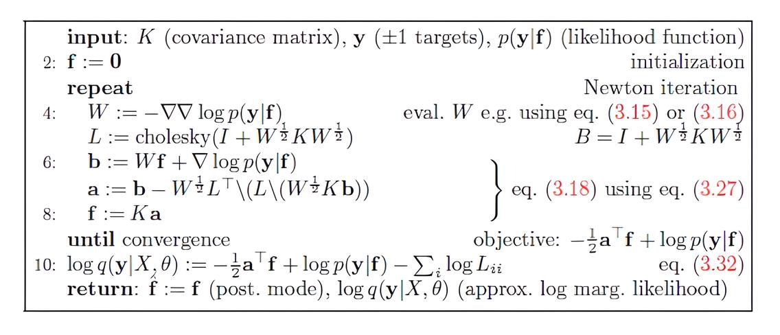
図1：f_hatとLMLのモードを探索するアルゴリズム3.1

最初に、Kカーネル共分散行列を計算します。より高速で安定した収束を実現するため、毎回ゼロベクトルから開始するのではなく、前回のハイパーパラメータ最適化の反復で得られたmu_f_trainをfの初期値として使用します。
ニュートン法を使用して、f_hatを反復的に更新します。
NLMLの計算：fのモードが収束した後（LMLの変化がm_tolerance未満になったとき）、NLMLの値をオプティマイザに渡します。

アルゴリズム5.1 GPML

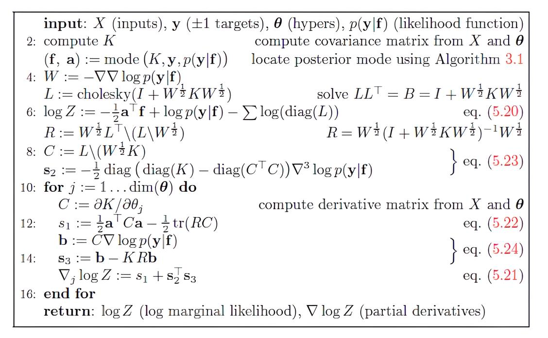
図2：LML勾配を計算するアルゴリズム5.1

カーネルのハイパーパラメータに関する勾配では、補助行列RとCの計算が必要です。R行列はcho_solveを使用して計算し、C行列はLinearEquationsSolutionTriangularを使用して計算します。
潜在関数の事後共分散行列は、学習データ上でΣf_train = K - C^TCとして計算されます。
各カーネルハイパーパラメータの勾配(dK_dtheta_j)は、明示的な項(s1)と暗黙的な項（s2、s3）で構成されます。s1の計算にはDiagonalTraceを使用して最適化を行い、s3にも連立方程式を解くためのcho_solveが含まれます。
尤度のハイパーパラメータに関する勾配は、対応するハイパーパラメータに関する対数尤度とそのヘッセ行列の微分を使用して計算します。このため、likelihoodオブジェクトのLogLikelihoodGradientParamメソッドとLogLikelihoodHessianDerivativeメソッドを使用します。

これで、基本的な構成要素（カーネル、尤度、推論手法）がすべて揃いました。それでは、ライブラリがどのように動作するかを実際に確認してみましょう。

合成データでライブラリをテストする

Gpsynthetic.mq5スクリプトを使用して、単純な合成データでライブラリをテストします。これにより、実装したメソッドが正しく動作していることを確認できます。

// --- Include the GP library ---
#include <GP/GP.mqh>

enum IntervalType
  {
   INTERVAL_F = 0, // Confidence interval of the f* latent function
   INTERVAL_Y = 1  // Confidence interval of y* observations
  };

enum Type_inference
  {
   Exact = 0,   // Exact Inference
   Laplace = 1  // Laplace Inference
  };

enum Type_Data
  {
   Regression = 0,    // Regression
   Classification = 1 // Classification
  };

//--- Input parameters
input IntervalType    interval_type  = INTERVAL_F;    // Interval type to display
input Type_Data       DataType       = Classification;
input Type_inference  inf            = Laplace ;        // Inference type

//+------------------------------------------------------------------+
//| Script program start function                                    |
//+------------------------------------------------------------------+
void OnStart()
  {
   string InpFileName1;
   string InpFileName2;
   string InpFileName3;
   string InpFileName4;

   if(DataType == Regression)
     {
      // Regression data
      InpFileName1 = "Data_Regression/X_train.csv";
      InpFileName2 = "Data_Regression/Y_train.csv";
      InpFileName3 = "Data_Regression/X_test.csv";
      InpFileName4 = "Data_Regression/Y_test.csv";
     }
   else
     {
      InpFileName1 = "Data_Classification/X.csv";  // 200
      InpFileName2 = "Data_Classification/y.csv";
      InpFileName3 = "Data_Classification/X_star.csv";
      InpFileName4 = "Data_Classification/y_star.csv";
     }

//----------- Dataset
   matrix x_train, y_train, x_test, y_test;
   CSVtoMatrix(InpFileName1,x_train);
   CSVtoMatrix(InpFileName2,y_train);
   CSVtoMatrix(InpFileName3,x_test);
   CSVtoMatrix(InpFileName4,y_test);

// Create label vectors from matrices
   vector y_train_ = y_train.Col(0);
   vector y_test_ = y_test.Col(0);

//--- 1. Create kernel objects
   IKernel* rbf = new RBFKernel(1,1);
// IKernel* linear = new LinearKernel(1.0);
// IKernel* periodic = new PeriodicKernel(1.0, 1.0, 5.8);

//--- 2. Combination of kernels (creation of a compound kernel)
// IKernel* functional_kernels_array[] = {rbf, linear, periodic};
// SumKernel* combined_functional_kernel = new SumKernel(functional_kernels_array);

//--- 3. Creating a likelihood object
   ILikelihood* likelihood = NULL; // Declare a pointer of the base type

   if(DataType == Regression)
     {
      likelihood = new GaussianLikelihood(1); // Assign the object
     }

   if(DataType == Classification)
     {
      likelihood = new LogitLikelihood();
     }

//--- 4. Create the inference object
   IInference* inference; // Declare a pointer to the interface
// Select the inference type:
   if(inf == Exact)
     {
      inference = new ExactInference();
     }
   else
     {
      inference = new LaplaceInference(100, 1e-10);
     }

//--- 5. Create an instance of the Gaussian Process model
   CREATE_GP_MODEL(gp_model, rbf, likelihood, inference,x_train, y_train_);
//  CREATE_GP_MODEL(gp_model, combined_functional_kernel, likelihood, inference,x_train, y_train_);
//--------------------------------------------------

   ulong start_time_fit = GetMicrosecondCount();
//--- 6. Hyperparameter optimization
   gp_model.Fit();
   ulong end_time_fit = GetMicrosecondCount();
   double elapsed_time_ms = (end_time_fit - start_time_fit) / 1000.0;
   Print(inference.GetName());
   Print("Fit execution time: ", StringFormat("%.3f", elapsed_time_ms), " ms");
   gp_model.PrintOptimizedKernelParameters();

//--- 7. Forecast for test points
   GPPredictionResult gp_predictions; // create a structure where the prediction results are to be set
   ulong start_time_predict = GetMicrosecondCount();
   gp_model.Predict(x_test, gp_predictions,PROBIT); // MONTE_CARLO,NUM_INTEGR,PROBIT
   ulong end_time_predict = GetMicrosecondCount();
   elapsed_time_ms = (end_time_predict - start_time_predict) / 1000.0;
   Print("Predict execution time: ", StringFormat("%.3f", elapsed_time_ms), " ms");

// --- 8. Classification results
   if(DataType == Classification)
     {
      DisplayClassificationResults(gp_predictions, y_test_);
     }
//--- 9. Regression Results
   if(DataType == Regression)
     {
      VisualizeGP(x_train, y_train, x_test, y_test_, gp_predictions, gp_model, 15);
     }

//--- 10. Releasing memory
   delete gp_model;
  }

選択したDataType（回帰または分類）に応じて、スクリプトは学習データとテストデータが格納されたCSVファイルへのパスを決定します。これらのファイルは、Files以下のData_RegressionまたはData_Classificationフォルダに配置されているものとします。

次に、カーネルオブジェクトを作成します。より複雑な共分散関数を構築するには、SumKernelやProductKernelなどの複合カーネルを使用できます。

続いて、選択したDataTypeに応じて尤度関数オブジェクト(ILikelihood)と推論オブジェクト(IInference)を作成します。

CREATE_GP_MODELマクロ（または同様のコンストラクタ）を使用してGPモデルを作成し、選択したカーネル、尤度関数、推論手法と学習データを関連付けます。

gp_model.Fit(int maxiter = 20)メソッドによって、モデルの学習処理が開始されます。このメソッドには、最大maxiter回の反復回数を設定するための新しいパラメータが追加されています。

学習が完了すると、gp_model.Predict()メソッドを使用して、新しい（テスト）データx_testに対する予測を実行します。予測結果（平均、共分散、確率/ラベル）は、GPPredictionResult構造体に格納されます。

分類では、予測モード（PROBIT、NUM_INTEGR、MONTE_CARLO）を選択できます。

その後、スクリプトは予測結果を出力します。

分類の場合は、DisplayClassificationResults()関数が呼び出され、精度指標と予測確率を計算します。
回帰の場合は、VisualizeGP()関数が結果の描画を担当します。

回帰では、y = sin(x) + 0.5 * x + noise(sigma = 0.1)という関数によって生成された合成データを使用します。この問題については、回帰を扱った記事ですでに説明しているため、ここでは詳しく取り上げません。ただし、解析的勾配とOpenBLASライブラリのメソッドを使用するようになってから、学習時間がどれほど改善されたかに注目してください。

二値分類では、XOR（排他的論理和）問題を表すデータを使用します。これは機械学習における古典的な問題であり、線形モデルの限界と、GPのような非線形アプローチを使用する必要性を示しています。

XORは、2つの二値入力（0または1）を受け取り、入力の一方だけが1の場合に1を、それ以外の場合に0を返す論理演算です。XORの真理値表：

XOR

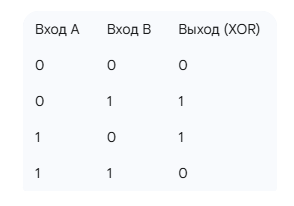
二値XOR分類の課題は、2つの入力（A、B）が与えられたとき、そのXOR出力（0または1）を予測するモデルを構築することです。ただし、今回のモデルは+1と-1のラベルのみを扱うため、ラベル0を-1に置き換えます。

XOR問題のデータは、次のように生成されます。2次元の入力点X (X=[x1,x2])を生成し、ある範囲（たとえば各軸で[-4,4]）にランダムに分布させます。これらの点のyラベルは、XORの論理に基づいて決定されます。

x1とx2の符号が同じ場合（両方が正、または両方が負）、積x1 * x2は正になります。この場合、ラベルは+1になります。
x1とx2の符号が異なる場合（一方が正で、もう一方が負）、積x1 * x2は負になります。この場合、ラベルは-1になります。

したがって、(+,+)と(-,-)の点はクラス+1に属し、(+,-)と(-,+)の点はクラス-1に属します。この問題では、非線形な依存関係に適切に対応し、GPによってこのようなクラスを効果的に分離できるため、RBFカーネルのみを使用します。

テストでは、学習に200個の観測値、新しい100個の点を精度のテストに使用しました。予測精度は98%となり、非線形分類問題の解決におけるGPの高い有効性を示しました。

GPRegressorインジケータ：GPによる時間方向の回帰

このインジケータは、不確実性を考慮した金融時系列の動的予測の例です。スライディングウィンドウを使用して学習サンプルを形成し、モデルを継続的に再学習することで、市場環境の変化に適応する仕組みを実装しています。

//+------------------------------------------------------------------+
//|                                                  GPRegressor.mq5 |
//|                                                           Eugene |
//|                                             https://www.mql5.com |
//+------------------------------------------------------------------+
#property copyright "Eugene"
#property link      "https://www.mql5.com"
#property version   "1.00"
// --- Include the GP library ---
#include <GP/GP.mqh>

#property indicator_chart_window
#property indicator_buffers 3
#property indicator_plots   2

// plot Predicted mean
#property indicator_label1  "Predicted mean"
#property indicator_type1   DRAW_LINE
#property indicator_color1  clrBlue
#property indicator_style1  STYLE_SOLID
#property indicator_width1  2

//--- plot Confidence interval
#property indicator_label2  "Confidence interval"
#property indicator_type2   DRAW_FILLING
#property indicator_color2   clrLightGray
#property indicator_width2  1

//--- Input parameters
input int    WindowLength   = 10;    // Window length for training the model
input int    calculate_bars = 100;   // History depth for calculation
input double zscore         = 1.96;  // z value for the interval (1.96 = 95%)
input bool   ShowRMSE       = false; // Show RMSE metric

//--- Buffers variables for rendering
double  ExtPredictionBuffer[]; // Buffer for predicted values
double  ExtUpperBandBuffer[];  // Buffer for the upper border of the confidence interval
double  ExtLowerBandBuffer[];  // Buffer for the lower border

//--- Global objects
GaussianProcess* g_gp_model       = NULL;
IKernel*         g_kernel         = NULL;
ILikelihood*     g_likelihood     = NULL;
IInference*      g_inference      = NULL;

//--- Global matrix for X_train temporary indices
matrix g_X_train;
//--- Global variables for RMSE data accumulation
vector gp_pred;
vector naive_pred;
vector y_true;
// Flag indicating whether the RMSE has already been calculated (for a one-time calculation)
bool rmse_calculated = false;
string comment;
double gp_rmse,naive_rmse;
//+------------------------------------------------------------------+
//| Custom indicator initialization function                         |
//+------------------------------------------------------------------+
int OnInit()
  {
   if(Bars(Symbol(), Period()) < WindowLength + calculate_bars)
     {
      PrintFormat("Error: Not enough bars to calculate. Minimum %d required. Available: %d",
                  WindowLength + calculate_bars, Bars(Symbol(), Period()));
      return(INIT_FAILED);
     }

   rmse_calculated = false; // Reset the flag on initialization/reinitialization
//--- Initialize global vectors for RMSE
   gp_pred.Resize(calculate_bars-1);
   naive_pred.Resize(calculate_bars-1);
   y_true.Resize(calculate_bars-1);

//--- indicator buffers mapping
   SetIndexBuffer(0, ExtPredictionBuffer, INDICATOR_DATA);
   SetIndexBuffer(1, ExtUpperBandBuffer,  INDICATOR_DATA);
   SetIndexBuffer(2, ExtLowerBandBuffer,  INDICATOR_DATA);

//--- Create kernel, likelihood, and inference method objects
   g_kernel = new RBFKernel(1.0, 1.0);
   if(g_kernel == NULL)
     {
      Print("Failed to create RBFKernel object");
      return(INIT_FAILED);
     }

   g_likelihood = new GaussianLikelihood(0.1);
   if(g_likelihood == NULL)
     {
      Print("Failed to create GaussianLikelihood object");
      delete g_kernel;
      return(INIT_FAILED);
     }

   g_inference = new ExactInference();
   if(g_inference == NULL)
     {
      Print("Failed to create ExactInference object");
      delete g_kernel;
      delete g_likelihood;
      return(INIT_FAILED);
     }

//--- Initialize the feature matrix X_train (one feature - time)
   g_X_train = matrix::Zeros(WindowLength, 1);
   for(int i = 0; i < WindowLength; i++)
     {
      g_X_train[i][0] = (double)(i + 1); // X = [1, 2, ..., WindowLength]
     }

//--- Create the GaussianProcess object
// Pass g_X_train and empty y_train
   vector initial_y_train = vector::Zeros(WindowLength);
   g_gp_model = new GaussianProcess(g_kernel, g_likelihood, g_inference, g_X_train, initial_y_train);
   if(g_gp_model == NULL)
     {
      Print("Failed to create GaussianProcess object");
      delete g_kernel;
      delete g_likelihood;
      delete g_inference;
      return(INIT_FAILED);
     }
   return(INIT_SUCCEEDED);
  }

//+------------------------------------------------------------------+
//|                                                                  |
//+------------------------------------------------------------------+
int OnCalculate(const int32_t rates_total,
                const int32_t prev_calculated,
                const datetime &time[],
                const double &open[],
                const double &high[],
                const double &low[],
                const double &close[],
                const long &tick_volume[],
                const long &volume[],
                const int32_t &spread[])
  {
// Check for sufficient number of bars
   if(rates_total < WindowLength)
     {
      Print("Error: Not enough bars to calculate. At least ", WindowLength, " is required, available: ", rates_total);
      return(0);
     }

   int start;
   if(prev_calculated == 0)
     {
      // Determine where to start the calculation.
      // calculate_bars - history depth to calculate.
      // MathMax(WindowLength, ...) ensures that we start no sooner than there is a full window of data.
      start = MathMax(WindowLength, rates_total - calculate_bars);
      // Initialize all buffers with EMPTY_VALUE
      ArrayInitialize(ExtPredictionBuffer, EMPTY_VALUE);
      ArrayInitialize(ExtUpperBandBuffer,  EMPTY_VALUE);
      ArrayInitialize(ExtLowerBandBuffer,  EMPTY_VALUE);
      // Set the start of rendering buffers
      PlotIndexSetInteger(0, PLOT_DRAW_BEGIN, start);
      PlotIndexSetInteger(1, PLOT_DRAW_BEGIN, start);
      PlotIndexSetInteger(2, PLOT_DRAW_BEGIN, start);
     }
   else
     {
      if(time[rates_total - 1] == time[prev_calculated - 1])
        {
         // This means that a new bar has NOT appeared.
         // We are on the same bar, just new ticks have arrived.
         return(rates_total);
        }
      // If the time of the last bar has changed, then a new closed bar has appeared.
      // Start calculation from prev_calculated to handle all new bars.
      start = prev_calculated;
     }

   for(int i = start; i < rates_total && !IsStopped(); i++)
     {
      // Check if there are enough bars to form a window
      if(i < WindowLength)
        {
         Print("Error: Not enough bars to form a window on bar ", i, ". Required: ", WindowLength, ", available: ", i);
         ExtPredictionBuffer[i] = EMPTY_VALUE;
         ExtUpperBandBuffer[i]  = EMPTY_VALUE;
         ExtLowerBandBuffer[i]  = EMPTY_VALUE;
         continue; // Skip this bar
        }

      // Form y vector from close[i-1], close[i-2], ..., close[i-WindowLength]
      // close[i-1]               - the newest bar in the window
      // close[i-WindowLength] - the oldest bar in the window
      vector y(WindowLength);
      for(int j = 0; j < WindowLength; j++)
        {
         y[WindowLength - 1 - j] = close[i - 1 - j];
        }
      //Print(" y = ", y[WindowLength-1]); // The newest bar in the window

      //--- Data standardization
      double mu_raw = y.Mean();
      // Print("mu_raw = ", mu_raw);
      double sigma_raw = y.Std();
      // Print("sigma_raw = ", sigma_raw);
      vector y_standardized = (y - mu_raw) / sigma_raw;

      //---  Set up training data
      g_gp_model.SetTrainingData(g_X_train, y_standardized);

      //--- Reset initial hyperparameters before Fit()
      vector initial_params(3);
      initial_params[0] = 1.0; // sigma_f (RBFKernel)
      initial_params[1] = 1.0; // length_scale (RBFKernel)
      initial_params[2] = 0.1; // sigma_n (GaussianLikelihood)
      g_gp_model.SetHyperparameters(initial_params);
      // vector params =  g_gp_model.GetCurrentHyperparameters();
      // Print(params);

      // ulong start_time_fit = GetMicrosecondCount();
      //--- Train the model
      if(!g_gp_model.Fit())
        {
         Print("Error: Failed to optimize GP hyperparameters for bar ", i);
         ExtPredictionBuffer[i] = EMPTY_VALUE;
         ExtUpperBandBuffer[i]  = EMPTY_VALUE;
         ExtLowerBandBuffer[i]  = EMPTY_VALUE;
         continue; // Skip the current bar
        }
      //ulong end_time_fit = GetMicrosecondCount();
      // double elapsed_time_ms = (end_time_fit - start_time_fit) / 1000.0;
      //Print("Fit execution time: ", StringFormat("%.3f", elapsed_time_ms), " мс");

      vector params =  g_gp_model.GetCurrentHyperparameters();
      double sigma_f      = params[0]; // sigma_f (RBFKernel)
      double length_scale = params[1]; // length_scale (RBFKernel)
      double sigma_n      = params[2]; // sigma_n (GaussianLikelihood)


      // --- Create a point for forecasting (X_star)
      // Predict the value for the next step after WindowLength
      matrix X_star = matrix::Zeros(1, 1);
      X_star[0][0] = (double)(WindowLength + 1);

      // --- Perform the prediction
      GPPredictionResult gp_predictions;
      if(!g_gp_model.Predict(X_star, gp_predictions))
        {
         Print("Error: Failed to get forecast from GP model for bar ", i);
         ExtPredictionBuffer[i] = EMPTY_VALUE;
         ExtUpperBandBuffer[i]  = EMPTY_VALUE;
         ExtLowerBandBuffer[i]  = EMPTY_VALUE;
         continue;
        }

      // ---
      double predicted_mean_st = gp_predictions.mu_f_star[0];
      // --- Perform the inverse transformation of the predicted mean value
      // back to the original price scale
      double predicted_mean = predicted_mean_st * sigma_raw + mu_raw;

      double sigma_f_star = gp_predictions.Sigma_f_star[0,0]; // dispersion (Σ) of f* signal
      double predicted_variance_st = gp_predictions.Sigma_y_star[0,0]; // dispersion(Σ) of y* observation
      // --- Perform the inverse dispersion transformation
      // The variance is scaled by the square of the standard deviation (sigma_raw) of the data,
      // used for standardization.
      double predicted_variance = predicted_variance_st * sigma_raw * sigma_raw;

      // Calculate the predicted confidence interval
      double std_predict = MathSqrt(predicted_variance);
      double upper_bound = predicted_mean + zscore * std_predict;
      double lower_bound = predicted_mean - zscore * std_predict;

      // --- Save the results to the indicator buffers for rendering
      ExtPredictionBuffer[i] = predicted_mean;
      ExtUpperBandBuffer[i]  = upper_bound;
      ExtLowerBandBuffer[i]  = lower_bound;

      comment = StringFormat("GP Regressor | Mean=%.5f | Upper=%.5f | Lower=%.5f |\n",
                             predicted_mean, upper_bound, lower_bound);
      comment+= StringFormat("Sigma_f = %.5f | Length_Scale = %.5f | Sigma_n = %.5f\n",sigma_f,length_scale,sigma_n);
      comment+= StringFormat("mu f* = %.5f | Σ y* = %.5f | Σ f*= %.5f",predicted_mean_st,predicted_variance_st,sigma_f_star);
      Comment(comment);
      // Debug output
      Print("Bar forecast ", i, ": Mean=", DoubleToString(predicted_mean, Digits()),
            " Upper=", DoubleToString(upper_bound, Digits()),
            " Lower=", DoubleToString(lower_bound, Digits()));
     }

// ---  Calculate RMSE to evaluate the efficiency of the GP forecast model compared to a simple "naive" forecast
   if(ShowRMSE && !rmse_calculated)
     {
      vector returns(calculate_bars-1);
      for(int j=0; j <calculate_bars-1;j++)
        {
         // true value
         y_true[j] = close[rates_total - calculate_bars + j];
         //Print("y_true[j]", y_true[j] );

         // GP forecast:
         gp_pred[j] = ExtPredictionBuffer[rates_total-calculate_bars + j];
         //Print("gp_pred[j]", gp_pred[j] );

         // "Naive" forecast (price tomorrow = price today):
         naive_pred[j] = close[rates_total - calculate_bars + j-1];
         // Print("naive_pred[j]", naive_pred[j] );

         returns[j] = close[rates_total - calculate_bars + j]  - close[rates_total - calculate_bars + j-1];
        }

      gp_rmse=gp_pred.RegressionMetric(y_true,REGRESSION_RMSE);
      naive_rmse=naive_pred.RegressionMetric(y_true,REGRESSION_RMSE);
      double std_returns = returns.Std(); // standard deviation of Close increments
      comment = comment + StringFormat("\nRMSE GP: %.5f | RMSE Naive: %.5f | StdDev Returns Close: %.5f ", gp_rmse, naive_rmse, std_returns);
      rmse_calculated = true;
     }
   Comment(comment);
//--- Return rates_total for the next call
   return(rates_total);
  }
//+------------------------------------------------------------------+
//| Custom indicator deinitialization function                       |
//+------------------------------------------------------------------+
void OnDeinit(const int reason)
  {
//--- Clear the comment on the chart
   Comment("");
//--- Free up the allocated memory for the GP object
   if(g_gp_model != NULL)
     {
      delete g_gp_model;
     }
  }
//+------------------------------------------------------------------+

入力パラメータ：

WindowLength：GPモデルの学習に使用するデータウィンドウの長さ（バー数）
calculate_bars：インジケータの計算と描画に使用する履歴の深さ
zscore：信頼区間を構築するための標準偏差の数（95%の場合は1.96など）
ShowRMSE：予測の二乗平均平方根誤差(RMSE)を表示するかどうかを指定するフラグ

初期化(OnInit)

グローバルオブジェクト：グローバルなカーネルオブジェクト(RBFKernel)、尤度関数(GaussianLikelihood)、推論手法(ExactInference)を作成して初期化します。
X_train特徴量：GPRegressorは、学習ウィンドウ内の時間インデックス（1からWindowLengthまで）をX入力として使用し、時間方向の回帰を実装します。
GaussianProcessモデル：g_gp_modelオブジェクトを指定された構成要素で初期化します。一方、y_trainは最初は空であり、動的に設定されます。

メイン計算ループ(OnCalculate)

データ生成：各バーで、直近の終値からWindowLength分のデータを抽出し、yベクトルを生成します。
データの標準化：GPの計算を数値的に安定させるため、yを標準化し、平均を0、分散を1にします。
モデルの更新と学習：

- 各ステップでyの目的データを更新します。g_X_trainの特徴量（時間インデックス）はウィンドウ内で一定のままです。
- 各学習前にハイパーパラメータを初期値にリセットします(g_gp_model.SetHyperparameters)。
- 現在のウィンドウで標準化された価格を使用してGPモデルを学習します(g_gp_model.Fit())。

予測：次のバーを予測するため、時間インデックスがWindowLength + 1となるX_star点を作成します。g_gp_model.Predict()メソッドが予測を実行し、標準化されたデータに対する平均(mu_f_star)と分散(Sigma_y_star)を返します。
標準化の解除：現在のウィンドウの平均(mu_raw)と標準偏差(sigma_raw)を使用して、予測された平均と分散を元の価格スケールに戻します。
信頼区間：変換後の平均と標準偏差、およびユーザーが指定した標準偏差の値zscoreに基づいて、信頼区間の上限と下限を計算します。

GPRegressor

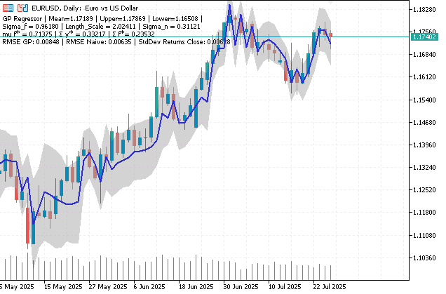
図3：回帰モデルの予測と95%信頼区間

RMSEインジケータの計算：

このインジケータは、ユーザーの要求に応じて、直近calculate_bars期間について、GPモデルによる予測と「ナイーブ」予測（明日の価格＝今日の価格）のRMSE統計を1回表示します。これにより、現在のモデルの有効性を客観的に評価できます。

たとえば、1分足のEURUSDで一般的に次のような指標になる場合があります。RMSE GP (0.00032) | RMSE Naive (0.00029)、また、終値の変化量の標準偏差(StdDev Returns Close)は0.00029です。

GPのRMSEがNaiveのRMSEより高いという事実は、分析対象期間においてGPモデルが単純なナイーブ予測よりも悪い結果になっていることを示します。さらに、RMSE NaiveとStdDev Returns Closeが等しいことは、将来の価格変化が過去の価格変化から独立しており、現在値が最良の予測となるランダムウォークの特徴です。

このことから、この時系列の区間には予測可能なパターンが存在しないか、あるいは時間だけを特徴量として使用している現在のGPモデルの構成では、ナイーブ予測を上回る有用な情報を抽出できていないと結論できます。

GPClassifierインジケータ：ガウス過程による分類

GPClassifierインジケータは、二値分類問題においてGPモデルを作成、学習し、予測するプロセスを示します。使用する特徴量は、過去のデータをスライディングウィンドウで処理して計算した終値の変化量です。NormalizeData関数を用いて特徴量行列を標準化し、モデルの学習を安定させます。

//+------------------------------------------------------------------+
//|                                                 GPClassifier.mq5 |
//|                                                           Eugene |
//|                                             https://www.mql5.com |
//+------------------------------------------------------------------+
#property copyright "Eugene"
#property link       "https://www.mql5.com"
#property version    "1.00"
// --- Include the GP library ---
#include <GP/GP.mqh>

#property indicator_chart_window
#property indicator_buffers 4
#property indicator_plots   2

// plot for predicted class "+1" (up arrows)
#property indicator_label1  "Predicted Class +1"
#property indicator_type1   DRAW_ARROW
#property indicator_color1  clrGreen
#property indicator_width1  1

// plot for predicted class "-1" (down arrows)
#property indicator_label2  "Predicted Class -1"
#property indicator_type2   DRAW_ARROW
#property indicator_color2  clrBlack
#property indicator_width2  1

//--- Input parameters
input int       WindowLength         = 10;    // Window length for training the GP model
input int       NumLags              = 1;     // Number of features
input int       calculate_bars       = 100;   // History depth for calculation
input double    ProbabilityThreshold = 0.5;   // Probability threshold 
input int       ArrowShiftPx         = 10;    // Arrow offset in pixels
input bool      ShowACCURACY         = false; // Show accuracy on the chart

//--- Buffers variables for rendering
double  ExtClassUpBuffer[];              // Buffer for displaying UP arrows
double  ExtClassDownBuffer[];            // Buffer for displaying DOWN arrows
double  ExtPredictedClassBuffer[];       // Buffer for storing predicted class labels
double  ExtPredictedProbabilityBuffer[]; // Buffer for storing predicted probabilities

//--- Global Gaussian process objects
GaussianProcess* g_gp_model    = NULL;
IKernel*         g_kernel      = NULL;
ILikelihood*     g_likelihood  = NULL;
IInference*      g_inference   = NULL;

//--- Global variables for classification metrics
bool accuracy_calculated = false; 
vector gp_pred,naive_pred,y_true,gp_accuracy,naive_accuracy;
string comment;
int currentsize;
//+------------------------------------------------------------------+
//| Custom indicator initialization function                         |
//+------------------------------------------------------------------+
int OnInit()
  {
   accuracy_calculated = false; // Reset the flag on initialization/reinitialization
//--- Initialize global vectors for Accuracy
   gp_pred.Resize(0);
   naive_pred.Resize(0);
   y_true.Resize(0);
   gp_accuracy.Resize(1);
   naive_accuracy.Resize(1);
   currentsize = 0;
//--- indicator buffers mapping
   SetIndexBuffer(0, ExtClassUpBuffer,     INDICATOR_DATA);    // For up arrows
   SetIndexBuffer(1, ExtClassDownBuffer,   INDICATOR_DATA);    // For down arrows
   SetIndexBuffer(2, ExtPredictedClassBuffer, INDICATOR_CALCULATIONS); //  to store predicted labels
   SetIndexBuffer(3, ExtPredictedProbabilityBuffer, INDICATOR_CALCULATIONS); // to store probabilities
// --- Set arrow symbols
   PlotIndexSetInteger(0, PLOT_ARROW, 225);   // Up arrow for buffer 0
   PlotIndexSetInteger(1, PLOT_ARROW, 226);   // Down arrow for buffer 1
// --- Set the arrow offset in pixels ---
// For the up arrows (buffer 0), use a negative offset so they are above High
   PlotIndexSetInteger(0, PLOT_ARROW_SHIFT, -ArrowShiftPx); // negative = up
// For the down arrows (buffer 1), use a positive offset so they are below Low
   PlotIndexSetInteger(1, PLOT_ARROW_SHIFT, ArrowShiftPx); // positive = down

// Add a check for the ratio of NumLags and WindowLength
   if(NumLags <= 0)
     {
      Print("Error: NumLags must be positive number");
      return(INIT_FAILED);
     }
   if(NumLags >= WindowLength)
     {
      Print("Error: NumLags (", NumLags, ") cannot exceed or be equal to WindowLength (", WindowLength, ").");
      return(INIT_FAILED);
     }

//--- Create kernel, likelihood, and inference method objects
   g_kernel = new RBFKernel(1.0, 1.0);
   if(g_kernel == NULL)
     {
      Print("Failed to create RBFKernel object");
      return(INIT_FAILED);
     }

   g_likelihood = new LogitLikelihood();
   if(g_likelihood == NULL)
     {
      Print("Failed to create LogitLikelihood object");
      delete g_kernel;
      return(INIT_FAILED);
     }

   g_inference = new LaplaceInference();
   if(g_inference == NULL)
     {
      Print("Failed to create ExactInference object");
      delete g_kernel;
      delete g_likelihood;
      return(INIT_FAILED);
     }
// --- Create the GaussianProcess model
// Pass empty matrices for X_train and y_train.
// They will be overridden in OnCalculate.
   g_gp_model = new GaussianProcess(g_kernel, g_likelihood, g_inference,matrix::Zeros(1,1), vector::Zeros(1));
   if(g_gp_model == NULL)
     {
      Print("Failed to create GaussianProcess object");
      delete g_kernel;
      delete g_likelihood;
      delete g_inference;
      return(INIT_FAILED);
     }
   return(INIT_SUCCEEDED);
  }
//+------------------------------------------------------------------+
//| Custom indicator iteration function                              |
//+------------------------------------------------------------------+
int OnCalculate(const int32_t rates_total,
                const int32_t prev_calculated,
                const datetime &time[],
                const double &open[],
                const double &high[],
                const double &low[],
                const double &close[],
                const long &tick_volume[],
                const long &volume[],
                const int32_t &spread[])
  {
// Check for sufficient number of bars
   if(rates_total < WindowLength + NumLags + 1)
     {
      Print("Error: Not enough bars to calculate. Required at least ", WindowLength + NumLags + 1, ", available: ", rates_total);
      return(0);
     }

   int start;
   if(prev_calculated == 0)
     {
      start = MathMax(WindowLength + NumLags + 1, rates_total - calculate_bars);
      // Initialize all EMPTY_VALUE buffers
      ArrayInitialize(ExtClassUpBuffer, EMPTY_VALUE);
      ArrayInitialize(ExtClassDownBuffer, EMPTY_VALUE);
      // Number of initial bars without rendering and values in DataWindow
      PlotIndexSetInteger(0, PLOT_DRAW_BEGIN, start);
      PlotIndexSetInteger(1, PLOT_DRAW_BEGIN, start);
     }
   else
     {
      if(time[rates_total - 1] == time[prev_calculated - 1])
        {
         return(rates_total);
        }
      start = prev_calculated;
     }

// --- Main forecast calculation loop
   for(int i = start; i < rates_total && !IsStopped(); i++)
     {
      // Check if there are enough bars to form X and y window
      if(i < WindowLength + NumLags + 1)
        {
         ExtClassUpBuffer[i] = EMPTY_VALUE;
         ExtClassDownBuffer[i] = EMPTY_VALUE;
         continue;
        }

      // --- Step 1: Generate training data (X_train and y_train) 
      matrix X_train = matrix::Zeros(WindowLength, NumLags);
      vector y_train = vector::Zeros(WindowLength);

      for(int j = 0; j < WindowLength; j++) 
        {
         // Calculate the bar index in the 'close' array for the current observation in the window.
         int idx = i - WindowLength + j;
         // Formation of features (lags) for the current observation (X_train[j] strings)
         for(int lag_idx = 0; lag_idx < NumLags; lag_idx++)
           {
            // Example:
            // lag_idx = 0: (close[idx - 1] - close[idx - 2]) - increment of the previous bar
            // lag_idx = 1: (close[idx - 2] - close[idx - 3]) - increment of the bar before last
            X_train[j,lag_idx] = close[idx - 1 - lag_idx] - close[idx - 2 - lag_idx];
           }

         // Y_train[j]: Binary label for price increment on idx bar.
         if(close[idx] - close[idx - 1] > 0)
           {
            y_train[j] = 1; // Price increased
           }
         else
           {
            y_train[j] = -1; // Price decreased or remained unchanged
           }

        }
      // Print(y_train);

      // --- Normalize X_train
      matrix X_train_norm;
      vector out_mean;
      vector out_std;
      if(!NormalizeData(X_train,X_train_norm,out_mean,out_std))
        {
         Print("Error: Failed to normalize feature matrix ", i);
         continue;
        }

      // --- Step 2: Feed data into the GP model
      g_gp_model.SetTrainingData(X_train_norm, y_train);

      // Reset initial hyperparameters before each Fit() training
      vector initial_params(2);
      initial_params[0] = 1.0; // sigma_f (RBFKernel)
      initial_params[1] = 1.0; // length_scale (RBFKernel)
      g_gp_model.SetHyperparameters(initial_params);

      // --- Step 3: Train the model
     //  ulong start_time_fit = GetMicrosecondCount();  
      if(!g_gp_model.Fit())
        {
         Print("Error: Failed to optimize GP hyperparameters for bar ", i);
         ExtClassUpBuffer[i] = EMPTY_VALUE;
         ExtClassDownBuffer[i] = EMPTY_VALUE;
         continue;
        }
       // ulong end_time_fit = GetMicrosecondCount();
      //  double elapsed_time_ms = (end_time_fit - start_time_fit) / 1000.0;
       // Print("Fit execution time: ", StringFormat("%.3f", elapsed_time_ms), " ms"); 

      // --- Step 4: Create a point for the X_star forecast
      // X_star - increment of prices of previous NumLags closed bars,
      // used to predict the movement of the current bar (i bar).
      matrix X_star = matrix::Zeros(1, NumLags);
      for(int lag_idx = 0; lag_idx < NumLags; lag_idx++)
        {
         X_star[0][lag_idx] = close[i - 1 - lag_idx] - close[i - 2 - lag_idx];
        }
      //  X_star should also be normalized using the same means and standard deviations,
      //  as for the corresponding X_train columns.
      for(int lag_idx = 0; lag_idx < NumLags; lag_idx++)
        {
         X_star[0][lag_idx] = (X_star[0][lag_idx] - out_mean[lag_idx]) / out_std[lag_idx];
        }

      // --- Step 5: Perform the prediction
      GPPredictionResult gp_predictions;
      if(!g_gp_model.Predict(X_star, gp_predictions))
        {
         Print("Error: Failed to get forecast from GP model for bar ", i);
         ExtClassUpBuffer[i] = EMPTY_VALUE;
         ExtClassDownBuffer[i] = EMPTY_VALUE;
         continue;
        }

      double predicted_probability = gp_predictions.predicted_probabilities[0]; // Probability for a single test point
      int predicted_class = (int)gp_predictions.predicted_labels[0]; // Label (+1 or -1)

      // --- Step 6: Save the results to the indicator buffers for rendering
      ExtClassUpBuffer[i] = EMPTY_VALUE;
      ExtClassDownBuffer[i] = EMPTY_VALUE;
      ExtPredictedClassBuffer[i] = predicted_class;
      ExtPredictedProbabilityBuffer[i] = predicted_probability;

      // Add the probability output and the number of features (lags) as a chart comment
      comment = StringFormat("GP Classifier (Lags: %d) | Probability(UP) = %.10f", NumLags, predicted_probability);
      Comment(comment);

      // If the predicted class is "+1" and the probability is above the given threshold
      if(predicted_class == 1 && predicted_probability > ProbabilityThreshold)
        {
         ExtClassUpBuffer[i] = high[i];
        }
      // If the predicted class is "-1" and the probability is above the given threshold
      else
         if(predicted_class == -1 && (1.0 - predicted_probability) > ProbabilityThreshold)
           {
            ExtClassDownBuffer[i] = low[i];
           }

      Print("Bar forecast ", i, ": Probability(UP)=" + DoubleToString(predicted_probability, 10) +
            ", Predicted Class=" + IntegerToString(predicted_class), " time: ", time[i]);
     }

// --- Calculate classification accuracy for assessing the efficiency of the GP predictive model in comparison 
//with a "naive" forecast.
   if(ShowACCURACY  && !accuracy_calculated)
     {
      for(int j=0; j <calculate_bars-1;j++)
        {
         // index to the current bar
         int bar_idx = rates_total - calculate_bars + j;

         if(ExtClassUpBuffer[bar_idx]!= EMPTY_VALUE || ExtClassDownBuffer[bar_idx] != EMPTY_VALUE)
           {
            currentsize = (int)gp_pred.Size();
            currentsize++;
            gp_pred.Resize(currentsize,100);
            naive_pred.Resize(currentsize,100);
            y_true.Resize(currentsize,100);

            // True label: count to the current bar
            if(close[bar_idx] - close[bar_idx - 1] > 0)
              {
               y_true[currentsize-1] = 1; // Price increased
              }
            else
              {
               y_true[currentsize-1] = -1; // Price decreased or remained unchanged
              }
            // Print("y_true",  y_true[currentsize-1] );

            // GP forecast: count to the current bar
            gp_pred[currentsize-1] = ExtPredictedClassBuffer[bar_idx];
            // Print(" gp_pred",  gp_pred[currentsize-1]);

            // "Naive" forecast: the "for tomorrow" bar label is equal to the "today" label
            if(close[bar_idx - 1] - close[bar_idx - 2] > 0)
              {
               naive_pred[currentsize-1] = 1;
              }
            else
              {
               naive_pred[currentsize-1] = -1;
              }
           }

        }

      if(!(int)gp_pred.Size()==0)
        {
         gp_accuracy=gp_pred.ClassificationMetric(y_true,CLASSIFICATION_ACCURACY);
         naive_accuracy=naive_pred.ClassificationMetric(y_true,CLASSIFICATION_ACCURACY);
         comment += StringFormat("\nGP Accuracy: %.2f %% | Naive Accuracy: %.2f %%", gp_accuracy[0], naive_accuracy[0]);
         comment += StringFormat("\nNumber of Filtered Signals: %d", (int)gp_pred.Size());
        }
      else
        {
         comment += StringFormat("\n No Signals for ProbabilityThreshold: %.4f ", ProbabilityThreshold);
        }
      accuracy_calculated = true;
     }
   Comment(comment); 
//--- Return rates_total for the next call
   return(rates_total);
  }

//+------------------------------------------------------------------+
//| Custom indicator deinitialization function                       |
//+------------------------------------------------------------------+
void OnDeinit(const int reason)
  {
// Clear the comment on the chart when deleting the indicator
   Comment("");

   if(g_gp_model != NULL)
     {
      delete g_gp_model;
     }
  }

入力パラメータ：

WindowLength：モデルの学習に使用するデータウィンドウの長さ。学習サンプルの観測数。
NumLags：ラグ（価格変化）の数。たとえば、NumLags = 1の場合、特徴量は直前のバーの価格変化のみとなります。NumLags = 3の場合、特徴量は直前3本のバーの価格変化となります。
calculate_bars：インジケータの計算および描画をおこなうチャート上の直近バーの本数。
ProbabilityThreshold：確率の閾値。予測された価格変動の確率がこの閾値を超えた場合、インジケータは上向きまたは下向きの矢印でシグナルを表示します。
ArrowShiftPx：バーの高値・安値から矢印をピクセル単位でずらす距離。
ShowACCURACY：チャート上に分類精度の指標を表示するかどうかを指定するフラグ。

OnInit()：GPモデルの初期化

RBFカーネル、尤度関数、推論手法を作成します。

g_kernel = new RBFKernel(1.0, 1.0)
g_likelihood = new LogitLikelihood()
g_inference = new LaplaceInference()

GaussianProcessモデルを作成します。

g_gp_model = new GaussianProcess(g_kernel, g_likelihood, g_inference, matrix::Zeros(1,1), vector::Zeros(1));
g_gp_modelオブジェクトは、X_trainとy_trainの学習データ用に空の初期行列を使用して作成されます。このデータはOnCalculate関数内で、各バーごとに動的に設定・更新されます。

OnCalculate()：メイン計算ループ

1. 十分な本数のバーが存在するかを確認します。計算を開始する前に、WindowLength、NumLags、および予測ラベル用の1本のバーを考慮し、学習ウィンドウを形成するのに十分な本数のバーがチャート上に存在することを確認します。

2. 学習データ（X_trainとy_train）の形成

X_trainの特徴量：各ステップで、スライディングウィンドウを使用してX_trainの特徴量行列を形成します。各行が1つの観測値を表し、各列には直前NumLags本のバーの価格変化（ラグ）が入ります。
y_trainのラベル：次のバーの価格変動方向を示す二値ラベルです。「1」（価格が上昇）または「-1」（価格が下落または変化なし）となります。

3. X_trainの正規化：特徴量行列を標準化し、GPの計算を数値的に安定させます。この処理で得られた平均値(out_mean)と標準偏差(out_std)は、予測点の正規化に使用するため保存されます。数値安定性のために特徴行列を標準化します。

4. GPモデルの更新と学習

g_gp_model.SetTrainingData(X_train_stdard, y_train)：各バーで学習データを更新します。
g_gp_model.SetHyperparameters(initial_params)：各新しいバーでカーネルのハイパーパラメータをリセットし、再最適化します。
g_gp_model.Fit()：現在のウィンドウで標準化されたデータを使用して学習を開始します。

5. 予測用の新しい点(X_star)の作成と正規化：out_meanとout_stdのベクトルを使用して正規化します。

6. 予測の実行：g_gp_model.Predict(X_star, gp_predictions) メソッドは、上昇方向への変動の予測確率(predicted_probabilities[0])と二値ラベル(predicted_labels[0])を返します。

7. 描画と出力：predicted_classとProbabilityThresholdに応じて、チャート上に上向きまたは下向きの矢印を描画します。予測確率と予測クラスに関する情報は、チャート上のコメントおよびログに表示されます。

GPClassifier

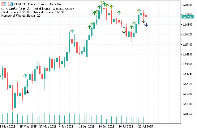
図4：GP Classifierインジケータの予測結果（RBFカーネル）

精度指標の計算(ShowACCURACY)

ShowACCURACYパラメータが有効になっている場合、インジケータは直近calculate_bars本について分類精度を1回計算し、GPモデルの予測と「ナイーブ」予測を比較します。

正解ラベル(y_true)は、実際の価格変動方向として定義されます。GP Prediction(gp_pred)はGPモデルによって予測されたラベルです。「ナイーブ」予測(naive_pred)は、次の価格変動方向が直前の変動方向と同じになると仮定します（たとえば、前のバーで価格が上昇した場合、ナイーブ予測も上昇となります）。

両モデルのCLASSIFICATION_ACCURACY指標（gp_accuracyとnaive_accuracy）を比較し、その結果をチャートコメントに表示します。これにより、単純なベンチマークと比較してGPモデルの性能を客観的に評価できます。

結論

本記事では、ガウス過程モデルの検討をひととおり終えました。理論的な構成要素を詳しく確認した後、回帰問題と分類問題の両方を解決できる基本的なライブラリを作成することができました。合成データを用いたテストでは、解析的勾配の効果的な利用や、高性能なOpenBLASライブラリの利用による数値的安定性と速度を含め、実装したライブラリの各コンポーネントが適切に動作することが確認されました。

GPRegressorおよびGPClassifierインジケータは、金融時系列をリアルタイムで動的に予測するためにGPを利用することが実用的に可能であることを示しました。また、回帰ではRMSE、分類ではAccuracyなどの指標を使用することで、モデルの性能を客観的に評価することができました。

しかし、ライブラリの実装はまだ理想的とは言えません。多くの努力を重ねたにもかかわらず、その速度はscikit-learnなどの確立されたソリューションよりも劣っています。これは、比較的低速なMinBleicオプティマイザーを使用していることが一因です。

したがって、今後のライブラリの改善には、以下のようなものが考えられます。

より効率的な勾配オプティマイザーの使用。特に、多数のハイパーパラメータを持つ問題において、現在の手法を効率面で大きく上回る高速なL-BFGSアルゴリズムが必要です。
Laplace近似におけるNewton法のより堅牢な実装。線形探索を追加することで、事後分布のモードをより効率的かつ確実に探索できるようになり、最終的な最適化の収束性を改善できます。
スパース手法の実装。現在のように完全行列を使用する方法とは異なり、スパース表現を使用することで、ライブラリを大幅に大きなデータ量で学習させることが可能となり、GPのスケーリングや応用に新たな可能性が開かれます。

最終的に、本稿の目的は、読者にガウス過程の基礎を紹介するとともに、より一般的な手法によって不当に影を潜めていると私が考えているベイズ機械学習ツールの力を示すことです。理論的基礎と、それをコードとして実際に実装した内容を通じて、この興味深いアプローチをさらに研究し、応用するきっかけとなれば幸いです。

記事で使用されているプログラム

#	名前	種類	詳細
1	GPClassifier.mq5	インジケータ	予測確率に基づいて1ステップ先の価格方向を分類する（オンライン学習）
2	GPRegressor.mq5	インジケータ	1ステップ先の価格と信頼区間を予測する（オンライン学習）
3	GPsynthetic.mq5	スクリプト	合成データを使用したGPモデルのテスト
4	GP.mqh	クラスライブラリ	カーネル、尤度関数、推論手法を組み合わせるGaussianProcessクラス、および最適化を担当するGPOptimizationObjectiveクラス
5	Inference.mqh	クラスライブラリ	推論手法を定義するIInferenceインターフェースとその実装
6	Kernels.mqh	クラスライブラリ	共分散カーネルのIKernelインターフェースとその実装
7	Likelihoods.mqh	クラスライブラリ	ILikelihoodインターフェースと尤度関数の実装
8	StructUtils.mqh	クラスライブラリ	補助関数とデータ構造
9	DataRegression	CSV	GPsynthetic.mq5スクリプトデータ
10	DataClassification	CSV	GPsynthetic.mq5スクリプトデータ

MetaQuotes Ltdによってロシア語から翻訳されました。
元の記事: https://www.mql5.com/ru/articles/19013

添付されたファイル |

ZIPをダウンロード

MQL5.zip (50.8 KB)

警告: これらの資料についてのすべての権利はMetaQuotes Ltd.が保有しています。これらの資料の全部または一部の複製や再プリントは禁じられています。

この記事はサイトのユーザーによって執筆されたものであり、著者の個人的な見解を反映しています。MetaQuotes Ltdは、提示された情報の正確性や、記載されているソリューション、戦略、または推奨事項の使用によって生じたいかなる結果についても責任を負いません。

Evgeniy Chernish

この著者による他の記事

最後のコメント | ディスカッションに移動 (4)

cemal | 27 6月 2026 において 16:34

こんにちは、

添付の画像のように、t+1などの予測ではなく、ラジアル基底関数を用いたGP回帰モデルで価格系列の分散を推定する方法について、具体例を示していただけますか？

Evgeniy Chernish | 27 6月 2026 において 18:47

cemal #:
こんにちは、

添付の画像のように、t+1などの予測を行う代わりに、ラジアル基底関数を用いたGP回帰モデルを使って価格系列の分散を調整する方法を、具体例を挙げてご説明いただけませんか？

こんにちは！

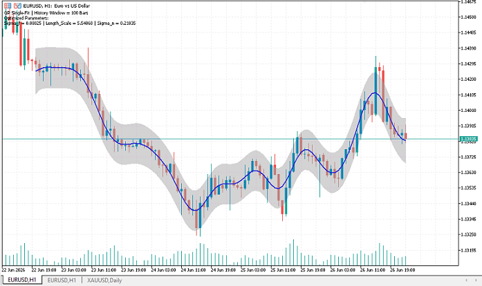
このような感じでしょうか？

GPR

これで、1ステップ先の予測ではなく、学習データセットの平均と分散が表示されるようになりました。

cemal | 28 6月 2026 において 22:40

本当にありがとうございます。とても親切ですね。

ガウス過程回帰モデルは、オンライン学習が可能で、データの平均や分散にリアルタイムで適応させることができますか？

Evgeniy Chernish | 29 6月 2026 において 10:17

cemal #:

本当にありがとうございます。とても親切ですね。

ガウス過程に基づく回帰モデルをオンラインで学習させ、データの平均値や分散にリアルタイムで適応させることが可能でしょうか？

はい、もちろんです。まさにそれがGPRegressor.m q5スクリプトの機能です。

EAのサンプル

一般的なMACDを使ったEAを例として、MQL4開発の原則を紹介します。

人工原子アルゴリズム(A3)

化学プロセスから着想を得たメタヒューリスティック最適化手法であるA3アルゴリズムをMQL5で実装します。調整可能なパラメータは2つだけであり、さらに小規模な集団を使用することで、十分な解の品質を維持しながら、高速に動作することを実現しています。

エラー 146 (「トレードコンテキストビジー」) と、その対処方法

この記事では、MT4において複数のEAの衝突をさける方法を扱います。ターミナルの操作、MQL4の基本的な使い方がわかる人にとって、役に立つでしょう。

市場シミュレーション：ポジション表示(IV)

ここからは、これまで完全に独立していたさまざまなコンポーネントやアプリケーションを、互いに連携させていきます。Chart Trade、マウスインジケータ、そしてエキスパートアドバイザー(EA)はすでに相互に接続されていましたが、これまでは、取引サーバー上で保有されているポジションをチャート上に直接表示する方法がありませんでした。特に、クロスオーダー方式を使用して管理されることの多いポジションを表示できるようになることで、ここからさまざまなアイデアや今後の実装につなげていくことが可能になります。まだこれらのコンポーネントを実際に動かし始めたばかりではありますが、今後の開発に向けた方向性はすでに見えてきています。