

Do My EA's Losses Come in Clusters? A Wald-Wolfowitz Runs Test for Trade Outcomes in MQL5
 64
 0

Contents
- Introduction
- What a run is
- How the pieces fit together
- Turning deal history into wins and losses: TradeSequence.mqh
- The runs test: RunsTest.mqh
- Streaks a trader would recognize: StreakStats.mqh
- Telling clustering from drift: BlockWinRates()
- Running it: the report script and the EA hook
- Checking the code: TestRunsTest.mq5
- Results on two of my EAs
- Checking the numbers outside MQL5
- Extending the module
- Limitations
- Conclusion
- References
- Attached files
Introduction
In an earlier article I built a per-setup trade ledger. It put a Wilson interval around the win rate of each entry type in an EA. In the review the moderator asked what assumptions that interval rests on. The interval treats the trades as Bernoulli trials: each trade wins with the same probability, and the result of one trade tells you nothing about the result of the next. I understood both conditions. I had never checked either of them on my own trades.
The second condition also sits under a rule I see in many EAs and trading plans. Stop for the day after 3 losses in a row, or cut the lot after a loss. A pause like this can serve several purposes, such as a daily loss limit or a cooling-off period for the trader. This article looks at one purpose only, the idea that the trade after a losing streak is more likely to lose. As a filter of that kind, the rule only helps if losses come in clusters. If they don't, the pause skips trades with the same chance of winning as any other trade.
Two articles on this site already point at the gap. Kayode Michael Oyetunde's article on hypothesis testing [1] warns that win and loss streaks make p-values look better than they are. The Monte Carlo stress test article [2] says it does not model serial correlation between trades. Neither of them tests for it.
This article implements the test as a small set of include files. They read the closed trades of an account or a tester run and convert them into a win/loss sequence in the order the trades closed. The Wald-Wolfowitz runs test [3] is applied to that sequence. Because traders think in streaks more than in runs, the module adds three streak checks: the longest losing streak, the loss rate of every trade after 3 or more losses, and the loss rate of the first trade after exactly 3 losses. Each check is compared with 10,000 shuffled orders of the same trades. A fourth check tests the other condition, a win rate that stays the same over time.
I run the module on two of my own EAs. The first is the SMC scalper from the ledger article on USDCAD, with five M1 runs in 2026, one M1 run in 2025, and one M15 run. The second is a gold version of the same idea, tested on 2025 and 2026 data. None of the checks detected dependence at the 5% level. The closest result, one setup losing more often right after 3 losses, did not repeat on the 2025 data. The article also shows how large an effect each check could have missed, and for some samples that effect is large.
What a run is
A run is a block of identical outcomes in a row. A sequence of eight trades that ended W W L L L W L W forms five runs: WW, LLL, W, L, and W.
If losses tend to follow losses and wins follow wins, the blocks get longer and there are fewer of them. If the outcomes flip more often than chance would give, the blocks get shorter and there are more of them. The test counts the runs and asks how unusual that count is for this many wins and losses, if every order of them were equally likely.
With n1 wins, n2 losses, and n = n1 + n2 trades, the expected number of runs under independence is 2 × n1 × n2 / n + 1. The variance is 2 × n1 × n2 × (2 × n1 × n2 − n) / (n² × (n − 1)). Fewer runs than expected points to clustering. More runs than expected points to alternation. I use a two-sided test, so either direction counts as evidence against independence.
Only the order of wins and losses matters. The test doesn't look at how much a trade won or lost, so a run of tiny losses and a run of large ones count the same. It also compares each trade only with its neighbor. Keep both limits in mind when you read the results.
How the pieces fit together
The module consists of four include files, two scripts, and a Python script. Fig. 1 shows how data moves through them.
Data flow of the runs test module
From the deal history to the journal and to the Python check
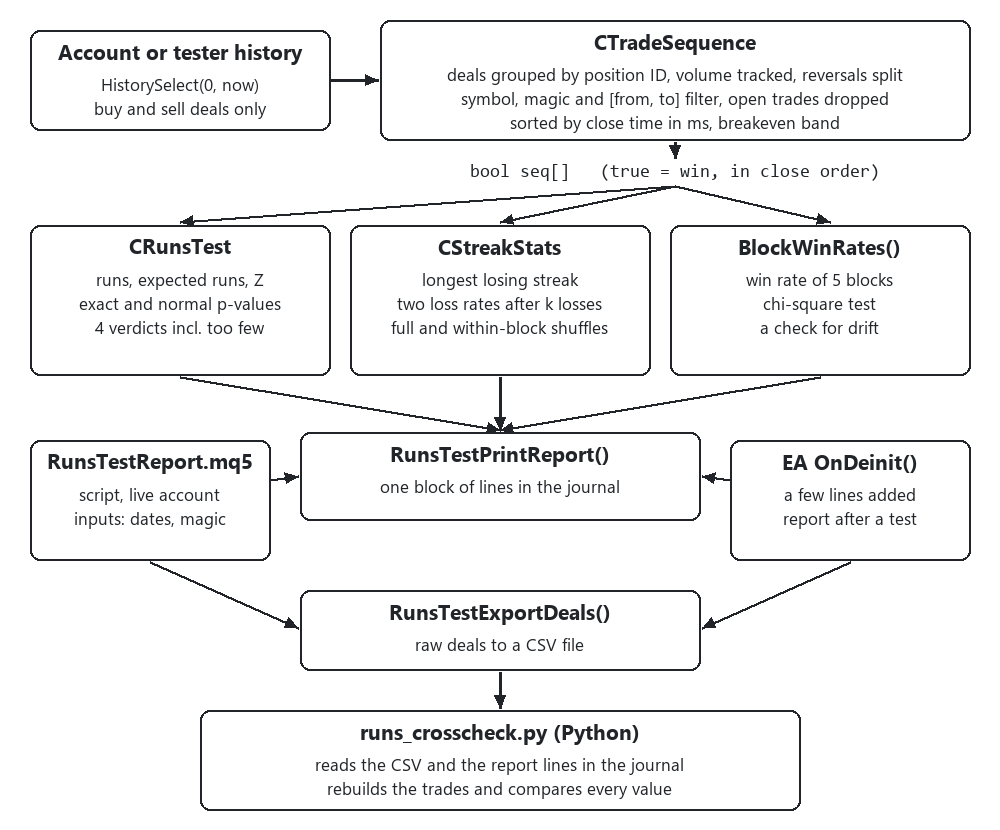
Fig. 1. Data flow from the deal history to the printed report and the Python cross-check
CTradeSequence reads the deals and produces one win or loss per closed trade. CRunsTest does the runs test. CStreakStats does the streak checks and the shuffling. BlockWinRates() splits the trades into five consecutive blocks and tests whether their win rates differ. RunsTestPrintReport() calls all of them and prints one block of lines. It can be called from the RunsTestReport.mq5 script on a live account, or from the OnDeinit() of any EA at the end of a test. RunsTestExportDeals() writes the raw deals to a CSV file, and runs_crosscheck.py rebuilds the whole report from that file without any MQL5 code.
Turning deal history into wins and losses: TradeSequence.mqh
One position, one outcome
MetaTrader keeps deals, not trades. A position opened once and closed in two parts leaves three deals: the entry and two exits. If every exit deal counted as a trade, one partial close would add an extra outcome and change the run count for no real reason. The moderator raised this exact problem with the history rebuild in my ledger class, so the grouping by DEAL_POSITION_ID [5] was there from the start.
The second detail is commission. On many accounts part of the commission is charged on the entry deal. A trade whose exit shows +0.50, with 0.70 charged on entry, lost 0.20. If you read only the exit deals it looks like a win. AddDeal() therefore adds the net of every deal to its trade, the entry included. It also keeps the volume that went in and the volume that came out. The volume is how Finalize() later decides whether a trade was closed.
//+------------------------------------------------------------------+
//| Add one deal to its trade                                        |
//+------------------------------------------------------------------+
void CTradeSequence::AddDeal(const long pos_id,const long time_msc,const long entry,
                             const double volume,const double pnl,const double costs,
                             const long magic,const string symbol)
  {
   int i=Find(pos_id);
   if(i<0)
      i=Append(pos_id,time_msc,magic,symbol);
//--- entry deal: volume in, and the magic the EA sent
   if(entry==DEAL_ENTRY_IN)
     {
      m_trades[i].net+=pnl+costs;
      m_trades[i].vol_in+=volume;
      if(!m_trades[i].has_entry)
        {
         m_trades[i].magic=magic;
         m_trades[i].has_entry=true;
        }
      return;
     }
//--- netting reversal: one deal closes the trade and opens the next one
   if(entry==DEAL_ENTRY_INOUT)
     {
      double closing=MathMax(m_trades[i].vol_in-m_trades[i].vol_out,0.0);
      double share  =(volume>0.0) ? MathMin(closing/volume,1.0) : 1.0;
      m_trades[i].net+=pnl+costs*share;
      m_trades[i].vol_out+=closing;
      m_trades[i].close_msc=time_msc;
      int j=Append(pos_id,time_msc,magic,symbol);
      m_trades[j].net=costs*(1.0-share);
      m_trades[j].vol_in=volume-closing;
      m_trades[j].has_entry=true;
      return;
     }
//--- exit deal (DEAL_ENTRY_OUT or DEAL_ENTRY_OUT_BY)
   m_trades[i].net+=pnl+costs;
   m_trades[i].vol_out+=volume;
   if(time_msc>m_trades[i].close_msc)
      m_trades[i].close_msc=time_msc;
  }
The magic number is taken from the entry deal. The EA sets the magic on the order it sends, and I didn't want to depend on what the exit deal carries when a stop-loss or take-profit closes the position. The test script feeds exits with magic 0 on purpose, to make sure the entry value is the one that counts.
On a netting account a reversal is a single DEAL_ENTRY_INOUT deal, and the position keeps its identifier. AddDeal() splits that deal in two. The part of its volume that closes the old trade takes the profit and its share of the costs, and the rest opens a new trade with the same position ID. Splitting the costs by volume is my own assumption. A unit test covers the split, but none of my test runs used a netting account.
After a reversal, two records share one position ID, so the lookup decides where the later deals go. Find() scans the records from the end and returns the latest one with that ID. Append() creates the second record.
//+------------------------------------------------------------------+
//| Index of the latest trade of a position ID, -1 if none           |
//+------------------------------------------------------------------+
int CTradeSequence::Find(const long pos_id) const
  {
//--- deals arrive in time order, so the match is usually near the end
   for(int i=m_count-1; i>=0; i--)
      if(m_trades[i].pos_id==pos_id)
         return(i);
   return(-1);
  }
//+------------------------------------------------------------------+
//| Start a new trade record and return its index                    |
//+------------------------------------------------------------------+
int CTradeSequence::Append(const long pos_id,const long time_msc,const long magic,const string symbol)
  {
   int i=m_count++;
   ArrayResize(m_trades,m_count,256);
   m_trades[i].pos_id=pos_id;
   m_trades[i].open_msc=time_msc;
   m_trades[i].close_msc=0;
   m_trades[i].net=0.0;
   m_trades[i].vol_in=0.0;
   m_trades[i].vol_out=0.0;
   m_trades[i].magic=magic;
   m_trades[i].symbol=symbol;
   m_trades[i].has_entry=false;
   return(i);
  }
LoadFromHistory() passes the deals to AddDeal() in history order. A DEAL_ENTRY_OUT that follows the reversal therefore reaches the new record, not the closed one. Case 18 of the test script covers this sequence. The reversal deal closes 1 lot and opens 2 lots. A separate DEAL_ENTRY_OUT then closes those 2 lots.
//--- 18. a netting reversal is split into two trades
   CTradeSequence tr;
   tr.AddDeal(7,100000,DEAL_ENTRY_IN,   1.0, 0.0,-1.0,5,"EURUSD");
   tr.AddDeal(7,200000,DEAL_ENTRY_INOUT,3.0,10.0,-3.0,5,"EURUSD");
   tr.AddDeal(7,300000,DEAL_ENTRY_OUT,  2.0,-5.0, 0.0,5,"EURUSD");
   tr.Finalize(0,1000,"",-1,-1);
   Check("18 reversal gives two trades",tr.Trades()==2,StringFormat("got %d",tr.Trades()));
   if(tr.Trades()==2)
     {
      CheckNear("18 first trade: profit and 1/3 of the costs",tr.Net(0),8.0,1e-9);
      CheckNear("18 second trade: 2/3 of the costs and its exit",tr.Net(1),-7.0,1e-9);
     }
The first trade holds the -1.0 entry cost, the 10.0 profit, and one-third of the -3.0 reversal cost. Their sum is 8.0. The second trade holds the other two-thirds of that cost and the -5.0 exit. Their sum is -7.0. If the exit reached the closed record, the second trade would stay open and the case would report one trade instead of two. The test output:
PASS  18 reversal gives two trades                 got 2
PASS  18 first trade: profit and 1/3 of the costs  got 8.000000000000, want 8.000000000000
PASS  18 second trade: 2/3 of the costs and its exit got -7.000000000000, want -7.000000000000
The time window
LoadFromHistory() selects the whole history, not the dates the user asks for. A trade opened before the start date still needs its entry deal, for the magic and for the commission. A trade that was partly closed before the end date and closed for good after it needs its later exits too. Without them, the partial result would look like a finished trade.
//+------------------------------------------------------------------+
//| Read buy and sell deals from the account or tester history       |
//+------------------------------------------------------------------+
bool CTradeSequence::LoadFromHistory(const datetime from,const datetime to,
                                     const string symbol,
                                     const long magic_from,const long magic_to)
  {
   Clear();
//--- the whole history: entries before "from" and exits after "to" both matter
   if(!HistorySelect(0,TimeCurrent()+86400))
      return(false);
   int total=HistoryDealsTotal();
   for(int i=0; i<total; i++)
     {
      ulong ticket=HistoryDealGetTicket(i);
      if(ticket==0)
         continue;
      long type=HistoryDealGetInteger(ticket,DEAL_TYPE);
      if(type!=DEAL_TYPE_BUY && type!=DEAL_TYPE_SELL)
         continue;
      AddDeal(HistoryDealGetInteger(ticket,DEAL_POSITION_ID),
              HistoryDealGetInteger(ticket,DEAL_TIME_MSC),
              HistoryDealGetInteger(ticket,DEAL_ENTRY),
              HistoryDealGetDouble(ticket,DEAL_VOLUME),
              HistoryDealGetDouble(ticket,DEAL_PROFIT)+HistoryDealGetDouble(ticket,DEAL_SWAP),
              HistoryDealGetDouble(ticket,DEAL_COMMISSION)+HistoryDealGetDouble(ticket,DEAL_FEE),
              HistoryDealGetInteger(ticket,DEAL_MAGIC),
              HistoryDealGetString(ticket,DEAL_SYMBOL));
     }
   Finalize(from,to,symbol,magic_from,magic_to);
   return(true);
  }
Finalize() applies the filters, the time window included. A trade whose volume is not fully closed, or whose last exit comes after the end date, had no known outcome at that date. It is dropped and counted as "open at the end".
//+------------------------------------------------------------------+
//| Keep trades fully closed inside [from, to], in close order       |
//+------------------------------------------------------------------+
void CTradeSequence::Finalize(const datetime from,const datetime to,const string symbol,
                              const long magic_from,const long magic_to)
  {
   long from_msc=(long)from*1000;
   long to_msc  =(long)to*1000+999;
   int  kept=0;
   m_still_open=0;
   for(int i=0; i<m_count; i++)
     {
      STradeOutcome t=m_trades[i];
      if(symbol!="" && t.symbol!=symbol)
         continue;
      if(magic_from>=0 && t.magic<magic_from)
         continue;
      if(magic_to>=0 && t.magic>magic_to)
         continue;
      //--- opened after the window
      if(t.open_msc>to_msc)
         continue;
      //--- still open, or closed for good only after "to": outcome unknown at "to"
      if(t.close_msc==0 || t.vol_out<t.vol_in-1e-8 || t.close_msc>to_msc)
        {
         m_still_open++;
         continue;
        }
      //--- closed before the window
      if(t.close_msc<from_msc)
         continue;
      m_trades[kept++]=t;
     }
   m_count=kept;
   ArrayResize(m_trades,m_count);
   SortByCloseTime();
  }
Breakeven trades and the order of trades
A trade that closes at zero, usually because the stop was moved to the entry price, is neither a win nor a loss. Build() leaves it out by default. It can also count it as a loss or as a win, since some people see a breakeven exit as a failed trade. The band around zero is half the smallest unit of the deposit currency, 0.005 on a USD account and 0.5 on an account in a currency without decimals. The net of a trade is a sum of several doubles, so it doesn't always land on exactly 0. SetBreakevenEps() sets a wider band for anyone who counts a trade within a few cents as breakeven.
//+------------------------------------------------------------------+
//| Win/loss array in close order, breakeven handled by the mode     |
//+------------------------------------------------------------------+
int CTradeSequence::Build(bool &seq[])
  {
   ArrayResize(seq,m_count);
   double eps=BreakevenEps();
   int    n=0;
   m_breakeven=0;
   for(int i=0; i<m_count; i++)
     {
      double net=m_trades[i].net;
      if(MathAbs(net)<=eps)
        {
         m_breakeven++;
         if(m_be_mode==BE_SKIP)
            continue;
         seq[n++]=(m_be_mode==BE_AS_WIN);
         continue;
        }
      seq[n++]=(net>0.0);
     }
   ArrayResize(seq,n);
   return(n);
  }
Leaving breakeven trades out has a side effect. Two trades that were not neighbors in time become neighbors in the sequence, and that can change the run count. In every backtest run in this article the report shows "breakeven 0", so the choice made no difference here. On an EA with many breakeven exits, compare BE_SKIP with BE_AS_LOSS before trusting either.
The order is the close time in milliseconds, from DEAL_TIME_MSC. When two trades close in the same millisecond, the lower position ID comes first, so the order never depends on how the history happens to be listed.
//+------------------------------------------------------------------+
//| Insertion sort by close time in ms, position ID breaks ties      |
//+------------------------------------------------------------------+
void CTradeSequence::SortByCloseTime(void)
  {
   for(int i=1; i<m_count; i++)
     {
      STradeOutcome t=m_trades[i];
      int j=i-1;
      while(j>=0 && (m_trades[j].close_msc>t.close_msc ||
                     (m_trades[j].close_msc==t.close_msc && m_trades[j].pos_id>t.pos_id)))
        {
         m_trades[j+1]=m_trades[j];
         j--;
        }
      m_trades[j+1]=t;
     }
  }
For an EA that holds one position at a time, close order is the only order there is. For an EA with overlapping trades it's a choice, and I come back to it under Limitations.
The runs test: RunsTest.mqh
Expected runs and the Z score
Compute() takes the counts and does all the work. It stores the moments, sums the exact tail probabilities from the probability of each possible run count, and works out the normal approximation next to them:
//+------------------------------------------------------------------+
//| Moments, exact tails and normal tails for given counts           |
//+------------------------------------------------------------------+
bool CRunsTest::Compute(const int n1,const int n2,const int runs)
  {
   m_n1=n1;
   m_n2=n2;
   m_runs=runs;
   m_ready=false;
   m_mean=0.0;
   m_var=0.0;
   m_p_low=1.0;
   m_p_high=1.0;
   m_p_low_norm=1.0;
   m_p_high_norm=1.0;
//--- with only wins or only losses there is nothing to test
   if(n1<1 || n2<1 || runs<2 || runs>MaxRuns())
      return(false);
//--- moments under independence
   double n=(double)n1+n2;
   double p=2.0*n1*n2;
   m_mean=p/n+1.0;
   m_var=p*(p-n)/(n*n*(n-1.0));
   m_log_total=LogChoose(n,n1);
//--- exact tails, summed from the pmf
   double low=0.0,high=0.0;
   int    max_runs=MaxRuns();
   for(int r=2; r<=max_runs; r++)
     {
      double pr=MathExp(LogPmf(r));
      if(r<=runs)
         low+=pr;
      if(r>=runs)
         high+=pr;
     }
   m_p_low=MathMin(low,1.0);
   m_p_high=MathMin(high,1.0);
//--- normal approximation with a 0.5 continuity correction
   if(m_var>0.0)
     {
      double sd=MathSqrt(m_var);
      m_p_low_norm=NormalCdf((runs+0.5-m_mean)/sd);
      m_p_high_norm=NormalCdf(-(runs-0.5-m_mean)/sd);
     }
   m_ready=true;
   return(true);
  }
The normal-approximation p-values use a 0.5 continuity correction, applied toward the mean. The Z() function returns the plain score without the correction, because that is the number people usually compare with 1.96.
Exact p-values, and a library function that returned NaN
The exact distribution of the run count is known. For an even count r = 2k the probability is 2 × C(n1 − 1, k − 1) × C(n2 − 1, k − 1) / C(n, n1). For an odd count r = 2k + 1 it is [C(n1 − 1, k) × C(n2 − 1, k − 1) + C(n1 − 1, k − 1) × C(n2 − 1, k)] / C(n, n1). The binomial coefficients get astronomically large for a few hundred trades, so everything is done in logarithms.
The standard library already has MathBinomialCoefficientLog() in Math\Stat\Math.mqh [6], so I used it. The first compile stopped with error 182, "ambiguous call to overloaded function". When I opened the library I found two versions of the function, one taking int arguments and one taking double. My call mixed a double and an int, so the compiler couldn't choose. That error was easy to fix. The int version builds the coefficient by multiplying in a long, and for large arguments the long overflows. The result is the logarithm of a negative number. In my test script C(62,31) through the int version prints "-nan(ind)", while the double version gives 40.681735.
All my other calls in that file passed int arguments. Once the first error was fixed, they would have compiled without a word and gone straight to the int version. The values 62 and 31 correspond to roughly 63 wins and 63 losses, which almost any EA history passes. So the test would have returned NaN on real data while working on every small example I tried by hand. Now every call goes through a helper that only accepts doubles:
//+------------------------------------------------------------------+
//| Log of C(n,k), always through the double overload                |
//+------------------------------------------------------------------+
double CRunsTest::LogChoose(const double n,const double k) const
  {
//--- the int overload works in a long and overflows from C(62,31) up
   return(MathBinomialCoefficientLog(n,k));
  }
//+------------------------------------------------------------------+
//| Log of the exact probability of r runs                           |
//+------------------------------------------------------------------+
double CRunsTest::LogPmf(const int r) const
  {
   int k=r/2;
//--- even r: k runs of each kind
   if(r%2==0)
      return(MathLog(2.0)+LogChoose(m_n1-1,k-1)
             +LogChoose(m_n2-1,k-1)-m_log_total);
//--- odd r: k+1 runs of one kind and k of the other
   double a=-DBL_MAX,b=-DBL_MAX;
   if(k<=m_n1-1 && k-1<=m_n2-1)
      a=LogChoose(m_n1-1,k)+LogChoose(m_n2-1,k-1);
   if(k-1<=m_n1-1 && k<=m_n2-1)
      b=LogChoose(m_n1-1,k-1)+LogChoose(m_n2-1,k);
   if(a==-DBL_MAX && b==-DBL_MAX)
      return(-DBL_MAX);
//--- log(e^a + e^b) without overflow
   double hi=MathMax(a,b),lo=MathMin(a,b);
   double sum=(lo==-DBL_MAX) ? hi : hi+MathLog(1.0+MathExp(lo-hi));
   return(sum-m_log_total);
  }
For an odd count one of the two terms can be impossible, for example when there aren't enough wins left for k + 1 win blocks. LogPmf() marks that term with -DBL_MAX and adds the two terms in log space without leaving it.
For large samples the exact version adds little. With 210 wins, 190 losses, and 185 runs, the exact lower tail is 0.066038 and the normal one 0.066078. With seven wins, five losses, and three runs the exact value is 0.0152 and the normal 0.0187, about 23% higher. People usually run a test like this on small samples, when they're worried about a new EA. So I compute the exact value everywhere and print the normal one next to it as a check.
Four verdicts
The moderator's review of my ledger article made one point I took into this design. "Not enough data" and "evidence against" are different answers and should not share a label. So the verdict has four states:
//+------------------------------------------------------------------+
//| Verdict of the runs test                                         |
//+------------------------------------------------------------------+
enum ENUM_RUNS_VERDICT
  {
   RUNS_TOO_FEW,                    // not enough wins or losses to judge
   RUNS_NOT_DETECTED,               // run count is inside the normal range
   RUNS_CLUSTERED,                  // fewer runs than chance: streaks or drift
   RUNS_ALTERNATING                 // more runs than chance: flip-flopping
  };
The wording of two of them is deliberate. A run count inside the normal range is reported as "no dependence detected by the runs test", not as "independent", because the test can only fail to find a pattern. A run count that is too low is reported as "clustering or drift", because a win rate that changes over time also produces fewer runs. The section on drift below shows how to tell the two apart.
The obvious way to decide "too few" is a fixed minimum number of trades. I kept one (10 wins and 10 losses by default), but it's a judgment call. The other rule is not. For some counts the test can't reject independence whatever the order is. With 4 wins and 4 losses, even the most extreme orders, LLLLWWWW or LWLWLWLW, give a two-sided p of 0.0571. Calling that result "not detected" would be misleading, because no detection was possible. MinAchievableP() computes the smallest p the counts allow, and if that is above alpha the verdict is "too few":
//+------------------------------------------------------------------+
//| Smallest two-sided p the test could reach with these counts      |
//+------------------------------------------------------------------+
double CRunsTest::MinAchievableP(void) const
  {
   if(!m_ready)
      return(1.0);
//--- the most extreme outcomes are 2 runs and the maximum runs
   double edge=MathMin(Pmf(2),Pmf(MaxRuns()));
   return(MathMin(1.0,2.0*edge));
  }
//+------------------------------------------------------------------+
//| Verdict at the chosen significance level                         |
//+------------------------------------------------------------------+
ENUM_RUNS_VERDICT CRunsTest::Verdict(void) const
  {
//--- too little data is kept apart from "not detected"
   if(!m_ready || m_n1<m_min_each || m_n2<m_min_each)
      return(RUNS_TOO_FEW);
   if(MinAchievableP()>m_alpha)
      return(RUNS_TOO_FEW);
//--- the tail the observed count falls in decides the direction
   if(PTwoSided()>m_alpha)
      return(RUNS_NOT_DETECTED);
   return(m_p_low<m_p_high ? RUNS_CLUSTERED : RUNS_ALTERNATING);
  }
The two-sided p-value is twice the smaller tail, capped at 1. Twice the smaller tail is one of several conventions for a discrete distribution that isn't symmetric. I picked it because it's the easiest one to check by hand.
Streaks a trader would recognize: StreakStats.mqh
The longest losing streak
A runs test answers a question most traders never ask. The question they do ask is closer to "I just lost 21 in a row. Is something broken?" CStreakStats answers that by shuffling. CStreakStats takes the same wins and losses and puts them in random order, 10,000 times by default. Then it counts how often a losing streak at least as long appears. If it happens often, the streak is what chance produces with that many losses.
The module uses a Fisher-Yates shuffle. MathRand() returns only 0 to 32767 [6], which can't pick a position in a history longer than that, so RandomIndex() combines two calls into 30 bits. Taking that number modulo the range would favor low indexes slightly, so values above the largest multiple of the range are rejected and drawn again. For 1,405 trades the bias this removes is about one part in a million, far below anything the report could show. The fix takes three lines. MathSrand() is set from an input seed so the same report can be reproduced exactly.
//+------------------------------------------------------------------+
//| Uniform index in [0, bound) from 30 random bits, no modulo bias  |
//+------------------------------------------------------------------+
uint CStreakStats::RandomIndex(const uint bound) const
  {
//--- MathRand() gives 15 bits, two calls give 30
   uint limit=(0x40000000/bound)*bound;
   uint r;
   do
      r=((uint)MathRand()<<15) | (uint)MathRand();
   while(r>=limit);
   return(r%bound);
  }
Each shuffle p-value adds 1 to both the numerator and the denominator. The observed order is one of the possible orders, and without this +1 a very unusual sequence would get a p of exactly 0 from a finite number of shuffles. With 10,000 shuffles the random error of a p near 0.05 is about 0.2 percentage points, and near 0.5 it is about 0.5 points. A two-sided p doubles one tail, so its error doubles too.
Two loss rates after 3 losses
The pause rule can be read in two ways, so the module measures two rates. LossRateAfter() takes every trade whose previous three trades were all losses, which means every trade after 3, 4, 5, or more losses in a row:
//+------------------------------------------------------------------+
//| Loss rate of every trade that follows k or more losses in a row  |
//+------------------------------------------------------------------+
bool CStreakStats::LossRateAfter(const bool &seq[],const int k,double &rate,int &n)
  {
   int losses=0,run=0;
   int size=ArraySize(seq);
   n=0;
   rate=0.0;
   for(int i=0; i<size; i++)
     {
      //--- run holds the losses in a row just before trade i
      if(run>=k)
        {
         n++;
         if(!seq[i])
            losses++;
        }
      run=seq[i] ? 0 : run+1;
     }
   if(n==0)
      return(false);
   rate=(double)losses/n;
   return(true);
  }
In a streak of 6 losses, the 4th, 5th, and 6th losses and the trade after them all count. Those observations overlap, so the rate can't be treated as a simple proportion with a binomial interval. The p-value is still valid, because every shuffle computes the same overlapping rate. Instead of a binomial interval, the report prints the range that holds 95% of the shuffled rates.
LossRateFirstAfter() counts only the trade right after the 3rd loss, once per losing streak. The first trade after the 3rd loss is the trade a rule of "skip one trade after 3 losses" would skip, and no trade is counted twice:
//+------------------------------------------------------------------+
//| Loss rate of the first trade after exactly k losses in a row     |
//+------------------------------------------------------------------+
bool CStreakStats::LossRateFirstAfter(const bool &seq[],const int k,double &rate,int &n)
  {
   int losses=0,run=0;
   int size=ArraySize(seq);
   n=0;
   rate=0.0;
   for(int i=0; i<size; i++)
     {
      //--- run==k happens once per losing streak, so no trade is counted twice
      if(run==k)
        {
         n++;
         if(!seq[i])
            losses++;
        }
      run=seq[i] ? 0 : run+1;
     }
   if(n==0)
      return(false);
   rate=(double)losses/n;
   return(true);
  }
My first thought was to compare these rates with the overall loss rate. Before writing the comparison I tried the shuffle on a toy sequence of 20 losses followed by 20 wins. In shuffled versions of it, with no dependence at all, I expected the loss rate after 3 or more losses to be a little under 50%. Three of the losses are already used up. The shuffled rate came out at 39.5% (test case 22 below).
This is the bias Miller and Sanjurjo described in their work on the hot hand [4]. In a finite sequence, the share of successes right after a streak of successes is biased downwards, and in short sequences the bias is large. Part of it is the used-up losses I expected. The rest comes from averaging a proportion over sequences in which only one or two trades follow a streak. For a trader it means that "68% of my trades after 3 losses were losses, and my loss rate is 65%" proves nothing on its own. On a short history the fair comparison is with the shuffled rate, and that is the number the report prints. On 1,405 trades the bias almost disappears, with an overall loss rate of 68.8% against a shuffled 68.6% in the results below. The bias matters most where people tend to look first, on a new EA with few trades.
The first time I ran the finished script on my demo account, which has only 24 closed trades, it showed the problem clearly. After 3 or more losses in a row came four trades, and three of those lost. That is 75.0%. The overall loss rate was 58% (14 of 24), which already makes 75% look high. The shuffled rate was 45.7%, and 95% of the shuffled rates fell between 0.0% and 85.7%. Against the shuffles p = 0.150. A sample of four trades is far too small to judge anything by.
Telling clustering from drift: BlockWinRates()
The runs test can't tell clustering from drift. If the win rate itself changes over time, for example when the market changes regime, wins bunch up in the good months and losses in the bad ones. Such drift produces fewer runs even when each trade is independent of the one before. A changing win rate also breaks the first condition of the Wilson interval. So the report has two checks for drift.
BlockWinRates() cuts the sequence into five consecutive blocks of equal size and runs a chi-square test of equal win rates across them, with four degrees of freedom. The p-value comes from MathCumulativeDistributionChiSquare() in the standard library [6]:
//+------------------------------------------------------------------+
//| Win rate of consecutive blocks and a chi-square test of equality |
//+------------------------------------------------------------------+
double BlockWinRates(const bool &seq[],const int blocks,double &rates[],double &chi2)
  {
   int n=ArraySize(seq);
   chi2=0.0;
   ArrayResize(rates,0);
   if(blocks<2 || n<2*blocks)
      return(1.0);
   ArrayResize(rates,blocks);
   int wins=0;
   for(int i=0; i<n; i++)
      if(seq[i])
         wins++;
   double pool=(double)wins/n;
   if(pool<=0.0 || pool>=1.0)
      return(1.0);
//--- 2 x blocks table: (wins - expected)^2 / (size * p * (1 - p)) summed
   for(int b=0; b<blocks; b++)
     {
      int lo=CStreakStats::BlockStart(b,n,blocks);
      int hi=CStreakStats::BlockStart(b+1,n,blocks);
      int w=0;
      for(int i=lo; i<hi; i++)
         if(seq[i])
            w++;
      int size=hi-lo;
      rates[b]=(double)w/size;
      chi2+=MathPow(w-size*pool,2)/(size*pool*(1.0-pool));
     }
   int err=0;
   return(MathCumulativeDistributionChiSquare(chi2,blocks-1.0,false,false,err));
  }
The second check repeats all the shuffle tests with the trades shuffled only inside each block. These within-block shuffles keep any difference in win rate between the blocks, and remove only the order inside each block. If the full shuffle flags a sequence and the within-block shuffle doesn't, drift between the blocks is a likelier explanation than clustering. Test case 23 shows the extreme case: 20 losses followed by 20 wins, cut into two blocks. The full shuffle flags the 20-trade losing streak with p 0.0005. Inside the blocks every order of the losses and of the wins looks the same, so the runs p is 1.000.
Both checks see a change between fifths of the history. Neither sees a change inside one block, a session effect, or a day-of-week effect. Five equal blocks are a default, set by the blocks field of the settings.
Running it: the report script and the EA hook
RunsTestPrintReport() takes a settings structure, loads the history, runs the checks, and prints one block. RunsTestReport.mq5 fills the structure from its inputs. On a live account you drop it on a chart and pick the dates, the symbol, and a magic range. A magic range rather than one value, because my ledger EA gives each setup its own magic number, base + 1 and base + 2. The whole EA is one range, and each setup is a range of one.
To print a report after a test, add one include line and a few lines to OnDeinit(). I applied this to the scalper. The full EA is attached as RunsTest_SMC.mq5, together with the CSetupLedger.mqh class it needs, so the M1 and M15 results can be repeated:
   //--- runs test on the same history: the whole EA, then each setup
   RunsTestExportDeals("RunsTest\\deals_"+_Symbol+"_"+EnumToString(_Period)+".csv");
   SRunsReportSettings rs;
   RunsReportDefaults(rs,_Symbol+" "+EnumToString(_Period)+", both setups");
   rs.symbol=_Symbol;
   rs.magic_from=(long)InpMagicNumber+SETUP_BULL_OB;
   rs.magic_to=(long)InpMagicNumber+SETUP_BEAR_OB;
   RunsTestPrintReport(rs);
   rs.title=_Symbol+" "+EnumToString(_Period)+", Bullish OB";
   rs.magic_to=rs.magic_from;
   RunsTestPrintReport(rs);
   rs.title=_Symbol+" "+EnumToString(_Period)+", Bearish OB";
   rs.magic_from=(long)InpMagicNumber+SETUP_BEAR_OB;
   rs.magic_to=rs.magic_from;
   RunsTestPrintReport(rs);
HistorySelect() works inside OnDeinit() during a test. In all my runs the report counted the same trades as the ledger's own final printout. RunsTestExportDeals() writes its CSV with FILE_COMMON. A file in the testing agent's own Files folder doesn't survive the end of the test, while the common folder does.
Checking the code: TestRunsTest.mq5
Before running anything on real trades I wanted the math pinned down. TestRunsTest.mq5 runs 23 numbered cases, 48 checks in total, and prints PASS or FAIL for each. The expected values come from two places. The small ones I worked out by hand. WWWWWLLLLL has two runs. Of the 252 possible orders of five wins and five losses, only two have two runs, so P(R ≤ 2) = 2/252. The larger ones come from a short Python script that uses exact integer arithmetic, with no floating point in the binomials at all. Cases 14 to 18 feed hand-made deals into CTradeSequence: partial closes, entry commission, the breakeven band, a trade that is still running at the end date, and a netting reversal. Part of the output:
PASS  6  P(R<=2), WWWWWLLLLL                       got 0.007936507937, want 0.007936507937
PASS  9  exact P(R<=185), 210 and 190              got 0.066037945076, want 0.066037945076
PASS  10 exact vs normal, 12 trades differ         exact 0.0152, normal 0.0187
PASS  11 4 and 4 cannot reject                     min p 0.0571, too few wins or losses to judge
PASS  13 int overload breaks at C(62,31)           int -nan(ind), double 40.681735
PASS  14 commission turns 2 into a loss            got -0.200000000000, want -0.200000000000
PASS  15 inside the band is breakeven              length 1, breakeven 1
PASS  17 partial close before "to" is not an outcome got 1 kept, 2 open at the end
PASS  18 first trade: profit and 1/3 of the costs  got 8.000000000000, want 8.000000000000
PASS  19 first trade after exactly 3 losses        got 2 streaks, 0.5000
PASS  21 streak p for 20 L then 20 W               p 0.0005
PASS  22 shuffled rate below overall rate          shuffled 0.395, overall 0.500
PASS  23 within-block runs p for drift only        p 1.000
48 passed, 0 failed
Case 13 tests the library, not my code. I left it in so that if MetaQuotes changes the int overload one day, the line will say so.
Results on two of my EAs
All runs: MetaTrader 5 build 6230, MetaQuotes-Demo hedging account, USD 10,000, leverage 1:100, random delay. Every input of each EA was written into the tester configuration with its default value. The EAs are unchanged apart from the report lines above. I searched every run's journal for "failed", "not enough money", "invalid stops", and "error". There were none.
USDCAD M1, five runs
The scalper traded USDCAD M1 from 1 January to 10 September 2026, every tick, five times. With random delay the trade count moves between runs, from 1,349 to 1,405 trades. The EA lost money in all five runs. The loss is already known from the ledger article and doesn't matter here. This is the report from run 1:
2026.09.09 23:59:59   === Runs test: USDCAD PERIOD_M1, both setups ===
2026.09.09 23:59:59   Filter: symbol USDCAD, magic 552001 to 552002, closed 1970.01.01 00:00:00 to 2026.09.10 23:59:59
2026.09.09 23:59:59   Trades 1405 (wins 439, losses 966), breakeven 0 (BE_SKIP, |net| <= 0.0050), open at the end 0
2026.09.09 23:59:59   Runs 595, expected 604.7, Z -0.60
2026.09.09 23:59:59   Exact p: fewer runs 0.2854, more runs 0.7380, two-sided 0.5708 (normal 0.5692)
2026.09.09 23:59:59   Verdict at alpha 0.05: no dependence detected by the runs test
2026.09.09 23:59:59   Longest losing streak 21, shuffles with one as long: p 0.147 (10000 shuffles)
2026.09.09 23:59:59   After 3 or more losses in a row: loss rate 69.4% (471 trades), shuffled 68.6% (95% range 65.1-71.9%), p 0.340
2026.09.09 23:59:59   First trade after exactly 3 losses: loss rate 69.7% (145 streaks), shuffled 68.8% (95% range 61.5-75.9%), p 0.404
2026.09.09 23:59:59   Win rate in 5 blocks: 31.7% 28.8% 31.3% 32.0% 32.4%, chi-square 1.04, p 0.904
2026.09.09 23:59:59   Within-block shuffles (5 blocks): runs p 0.517, streak p 0.130, after p 0.291, first p 0.404
The ledger printed Bullish OB 241/556 and Bearish OB 198/410 (wins/losses) for the same run. 797 + 608 = 1,405 trades, and 241 + 198 = 439 wins. The setup nets, -6,138.98 and -1,180.81, add up to -7,319.79, which is the drop from 10,000.00 to the final balance of 2,680.21. The two tools read the same history.
The observed 595 runs against 604.7 expected is a shortfall of about 10 runs. Fig. 2 shows where 595 sits in the exact distribution for these counts. The zigzag between neighboring bars is real. When the numbers of wins and losses differ, even and odd run counts have different probabilities.
Exact distribution of runs for 439 wins and 966 losses
USDCAD M1, run 1 of the SMC scalper
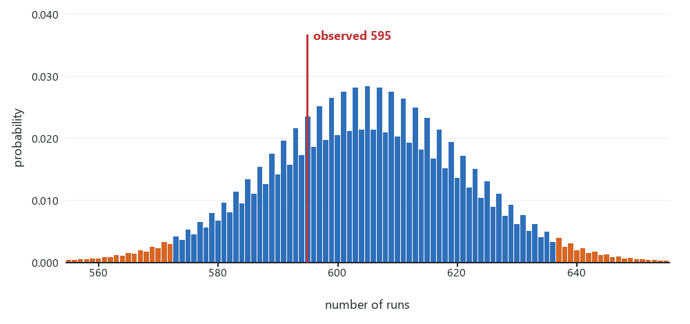
Fig. 2. Exact distribution of the number of runs for 439 wins and 966 losses. Orange bars are the 2.5% tails on each side (below 573 and above 636). The observed 595 is inside the middle range
Before the test, the 21-trade losing streak looked like the most worrying number. In 14.7% of 10,000 shuffles in MQL5 there was a losing streak at least that long. Fig. 3 repeats the shuffle in Python with its own random numbers, where the share is 14.4%. With 966 losses out of 1,405 trades, a streak of 21 is unusual but far from rare.
Longest losing streak in 10,000 shuffles
The same 439 wins and 966 losses in random order
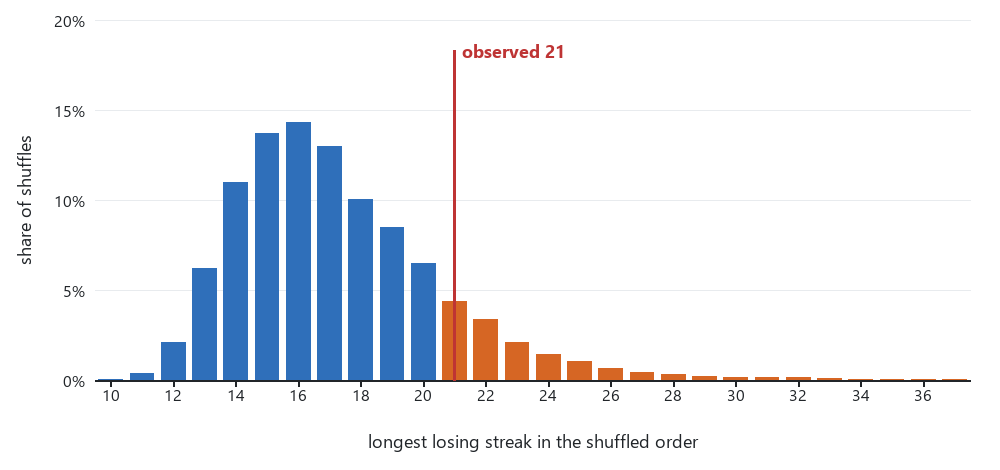
Fig. 3. Longest losing streak in 10,000 shuffles of the same 439 wins and 966 losses, drawn in Python. Orange: 21 or longer, 14.4% of shuffles. The MQL5 report gave 14.7%
All five runs, first the runs test and the drift test:
| Run | Trades | Wins/losses | Runs | Expected | Z | Exact p | Drift p (five blocks) |
|---|---|---|---|---|---|---|---|
| 1 | 1,405 | 439/966 | 595 | 604.7 | -0.60 | 0.5708 | 0.904 |
| 2 | 1,349 | 425/924 | 577 | 583.2 | -0.39 | 0.7199 | 0.750 |
| 3 | 1,357 | 427/930 | 579 | 586.3 | -0.46 | 0.6710 | 0.850 |
| 4 | 1,349 | 425/924 | 577 | 583.2 | -0.39 | 0.7199 | 0.800 |
| 5 | 1,365 | 428/937 | 581 | 588.6 | -0.48 | 0.6566 | 0.909 |
Then the streak checks. Each rate is followed by the shuffled rate and the p-value:
| Run | Longest losing streak (p) | After 3 or more losses | First trade after exactly 3 losses | Runs p, within-block shuffles |
|---|---|---|---|---|
| 1 | 21 (0.147) | 69.4%, 68.6% (0.340) | 69.7%, 68.8% (0.404) | 0.517 |
| 2 | 18 (0.365) | 68.8%, 68.4% (0.411) | 70.5%, 68.6% (0.309) | 0.680 |
| 3 | 18 (0.380) | 69.0%, 68.4% (0.395) | 70.7%, 68.6% (0.285) | 0.606 |
| 4 | 18 (0.367) | 68.8%, 68.4% (0.413) | 71.2%, 68.5% (0.235) | 0.666 |
| 5 | 18 (0.386) | 68.7%, 68.6% (0.489) | 71.1%, 68.7% (0.258) | 0.594 |
Every run has a few runs fewer than expected, with Z between -0.39 and -0.60, far from anything the test would call a result. I wouldn't read anything into the sign. The five runs trade the same signals on the same data, so they are reruns of one test with different execution delays, not five independent samples. Runs 2 and 4 even ended with the same counts, although their trade lists differ.
Each setup on its own
Clustering in the whole EA could hide in one setup and be diluted by the other, so the hook also reports each magic number separately. Run 1:
| Setup | Trades | Wins/losses | Runs | Expected | Z | Exact p | Drift p (five blocks) |
|---|---|---|---|---|---|---|---|
| Bullish OB | 797 | 241/556 | 327 | 337.3 | -0.86 | 0.4154 | 0.695 |
| Bearish OB | 608 | 198/410 | 261 | 268.0 | -0.65 | 0.5476 | 0.942 |
| Setup | Longest losing streak (p) | After 3 or more losses | First trade after exactly 3 losses | Runs p, within-block shuffles |
|---|---|---|---|---|
| Bullish OB | 20 (0.147) | 67.9%, 69.5% (0.769) | 64.4%, 69.8% (0.865) | 0.384 |
| Bearish OB | 11 (0.943) | 67.2%, 67.2% (0.519) | 76.2%, 67.6% (0.062) | 0.458 |
In runs 2 to 5 the exact p-values were 0.40 to 0.48 for Bullish OB and 0.71 to 0.86 for Bearish OB. After 3 or more losses, Bullish OB lost less often than its shuffled rate in all five runs. Bearish OB did so in four runs and matched it in one.
The first trade after exactly 3 losses is the one result in this article that leans the way the pause rule assumes. On Bearish OB that trade lost 73.8% to 76.2% of the time across the five runs, against a shuffled 67.4% to 67.9%, with p between 0.062 and 0.133. The rate covers 60 to 63 losing streaks. Fig. 4 shows run 1 against its shuffles.
First trade after exactly 3 losses, Bearish OB
USDCAD M1 2026, run 1, observed rate against 10,000 shuffles
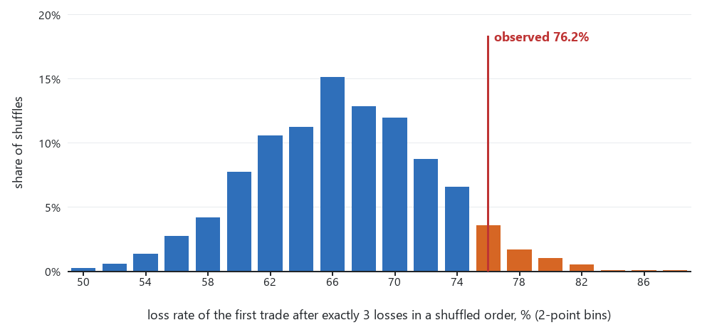
Fig. 4. Loss rate of the first trade after exactly 3 losses in 10,000 shuffles of the Bearish OB trades, drawn in Python. The red line marks the observed 76.2% over 63 streaks. 6.7% of the Python shuffles reached it or more, and the MQL5 report gave p 0.062. Orange: the bins from 76% up
The five runs are reruns of one data set, so a lean that shows up in all of them is one observation repeated, not five. The Bearish OB result was also one of more than 200 p-values in this article. A result like this needs data the check has never seen. So I ran the same EA on USDCAD M1 for all of 2025. No runs test report for this EA on 2025 USDCAD data existed before this run:
| USDCAD M1 2025 | Trades | Wins/losses | Exact p | Drift p | After 3 or more losses | First trade after exactly 3 losses |
|---|---|---|---|---|---|---|
| Both setups | 1,366 | 390/976 | 0.5043 | 0.839 | 70.7%, 71.4% (0.674) | 71.1%, 71.5% (0.540) |
| Bullish OB | 774 | 227/547 | 0.7492 | 0.746 | 72.1%, 70.5% (0.239) | 74.7%, 70.8% (0.220) |
| Bearish OB | 592 | 163/429 | 0.8604 | 0.559 | 69.4%, 72.3% (0.890) | 66.7%, 72.6% (0.873) |
In 2025 the first trade after 3 Bearish OB losses lost less often than the shuffled rate, 66.7% against 72.6%. The 2026 lean did not repeat. The other setup moved the opposite way, also without reaching significance. Read together, the two years look like noise around the shuffled rate.
Drift
Fig. 5 shows the five block win rates of run 1. Bullish OB drops to 25.8% in the second block and recovers. The same dip, between 24.8% and 25.8%, appears in all five runs, which is expected when they trade the same signals. None of the chi-square tests came close to significance, with p between 0.383 and 0.986 across the 15 report blocks of the five runs. The within-block runs p-values ranged from 0.384 to 0.739, so removing the drift between blocks didn't bring any result near significance. Nothing in these runs suggests that drift hid or created a result.
Win rate of five consecutive blocks
USDCAD M1 2026, run 1, both setups and each setup
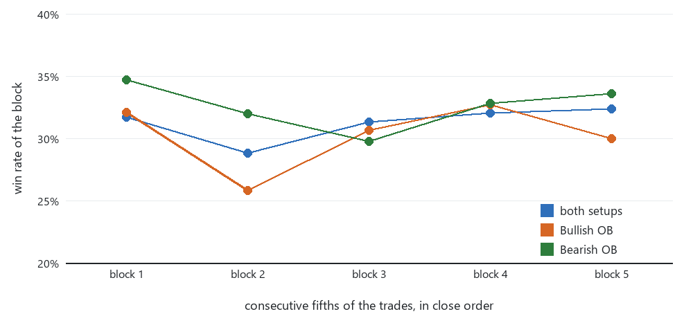
Fig. 5. Win rate of each fifth of the trades in close order, rebuilt in Python from the deals file of run 1. Chi-square p: both setups 0.904, Bullish OB 0.695, Bearish OB 0.942
M15 and gold
| Test | Trades | Wins/losses | Runs | Expected | Z | Exact p | Drift p (five blocks) |
|---|---|---|---|---|---|---|---|
| USDCAD M15, 2026.01.01-09.10, every tick | 131 | 47/84 | 65 | 61.3 | 0.71 | 0.5462 | 0.535 |
| XAUUSD M15, 2025, every tick | 175 | 64/111 | 86 | 82.2 | 0.62 | 0.5865 | 0.768 |
| XAUUSD M15, 2026.01.01-09.20, real ticks | 127 | 47/80 | 66 | 60.2 | 1.11 | 0.3090 | 0.279 |
| Test | Longest losing streak (p) | After 3 or more losses, 95% of shuffles | First trade after exactly 3 losses |
|---|---|---|---|
| USDCAD M15 | 8 (0.778) | 65.6%, 62.6% (0.372), 46.7% to 75.6%, 32 trades | 63.6%, 64.3% (0.545), 11 streaks |
| XAUUSD 2025 | 9 (0.676) | 67.5%, 62.4% (0.206), 48.6% to 73.9%, 40 trades | 71.4%, 63.9% (0.270), 14 streaks |
| XAUUSD 2026 | 7 (0.900) | 60.0%, 61.5% (0.615), 44.4% to 75.6%, 25 trades | 60.0%, 63.5% (0.613), 10 streaks |
These have more runs than expected rather than fewer, and again nothing close to significant. The rates after 3 losses rest on 25 to 40 trades, or 10 to 14 streaks, and the 95% ranges of the shuffled rates are 25 to 31 percentage points wide. Estimates that loose can't support a conclusion either way. The shuffled column also shows the bias from the toy example. Comparing 67.5% with the plain 2025 gold loss rate of 63.4% (111 of 175) would have looked like a small clustering effect. Against the shuffled 62.4% it's p = 0.206.
How much dependence the checks could have seen
"Not detected" is only worth something if the check had a fair chance of detecting an effect. To measure that, runs_crosscheck.py simulates trades with a known dependence. A loss raises the chance that the next trade also loses by 5 or by 10 percentage points (points from here on). The overall loss rate stays the same as in the real trades. For a loss rate of 69%, a 5-point effect means 74% after a loss. The script runs each check on 2,000 such sequences at the 5% level and counts how often it flags them. The critical values come from shuffles of the real counts.
| Sample | Trades | Runs count | Longest losing streak | After 3 or more losses | First after exactly 3 |
|---|---|---|---|---|---|
| M1 run 1, both setups | 1,405 | 100%/100% | 15%/48% | 87%/100% | 41%/86% |
| M1 run 1, Bullish OB | 797 | 98%/100% | 17%/46% | 70%/100% | 26%/65% |
| M1 run 1, Bearish OB | 608 | 92%/100% | 16%/43% | 59%/97% | 19%/50% |
| USDCAD M15, both setups | 131 | 37%/88% | 13%/26% | 22%/48% | 9%/17% |
| USDCAD M15, Bullish OB | 74 | 25%/67% | 16%/30% | 19%/38% | 0%/0% |
| USDCAD M15, Bearish OB | 57 | 21%/56% | 14%/26% | 15%/29% | 0%/0% |
| XAUUSD 2025 | 175 | 44%/93% | 14%/31% | 25%/55% | 10%/19% |
| XAUUSD 2026 | 127 | 34%/86% | 9%/22% | 20%/46% | 11%/19% |
Each cell shows the share of sequences flagged for a 5-point and a 10-point effect. Fig. 6 shows the 10-point column for three of the samples.
Power of the four checks at a 10-point effect
Share of 2,000 simulated sequences each check flags at the 5% level
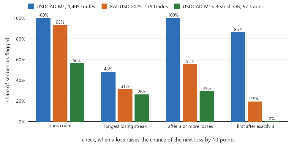
Fig. 6. Share of simulated sequences flagged by each check when a loss raises the chance of the next loss by 10 points, for USDCAD M1 run 1, XAUUSD 2025, and USDCAD M15 Bearish OB
Three things stand out. On M1 the runs count would almost certainly have flagged a 5-point effect, in the whole EA and in each setup, so "not detected" there means something. The rate after 3 or more losses caught the same effect in 59% to 87% of the sequences. The longest losing streak is the weakest check everywhere, below 50% even at 10 points, so a long streak alone says little about clustering. On M15 and gold every check misses most 5-point effects. On the M15 setups the first-trade check can never flag anything. With five or six streaks the shuffled rate reaches 100% too often, the same problem MinAchievableP() catches for the run count.
For the pause rule, this is what I take from it. On these two EAs, over these periods, none of the checks found the trade after a losing streak to lose more often than chance gives. On M1 the checks were strong enough to see a 5-point effect, and on M15 and gold they were not. These results don't prove that a pause rule is useless. They show that the data gives no support for a pause as a filter on these two EAs, and that the M15 and gold samples are too small to settle the question. A pause kept for risk reasons is outside what this test measures.
Checking the numbers outside MQL5
Numbers printed by the same code that computed them can be wrong in the same way twice. So runs_crosscheck.py recomputes the report in Python with the standard library only, starting from the raw deals. It is a consistency check, a second implementation of my own rules, not independent validation. It reads the report blocks from a tester log or a journal, and the deals from the CSV that RunsTestExportDeals() writes. For each block it applies the printed filter and rebuilds the trades with its own code, including the volume check, the reversal split, and the millisecond order. Then it recomputes 17 values: the trade count, wins, losses, breakeven trades, runs, expected runs, Z, both two-sided p-values, the longest streak, both rates after 3 losses with their counts, the five block win rates, the chi-square, and its p-value. The exact p uses integer binomial coefficients, with no floating point. This is its output for M1 run 1, M15, and both gold runs, with the power simulation:
rt5_M1_1_log.txt + deals5_M1_1.csv: 2810 buy and sell deals
  USDCAD PERIOD_M1, both setups: 17 of 17 values match the report
    1405 trades (439 W, 966 L), runs 595, exact p 0.5708, longest 21, after 69.4%, first 69.7%
    shuffles Python/MQL5: streak p 0.143/0.147, after p 0.335/0.340, first p 0.413/0.404
    within blocks Python/MQL5: runs p 0.509/0.517, streak p 0.127/0.130
  USDCAD PERIOD_M1, Bullish OB: 17 of 17 values match the report
    797 trades (241 W, 556 L), runs 327, exact p 0.4154, longest 20, after 67.9%, first 64.4%
    shuffles Python/MQL5: streak p 0.154/0.147, after p 0.780/0.769, first p 0.870/0.865
    within blocks Python/MQL5: runs p 0.375/0.384, streak p 0.136/0.140
  USDCAD PERIOD_M1, Bearish OB: 17 of 17 values match the report
    608 trades (198 W, 410 L), runs 261, exact p 0.5476, longest 11, after 67.2%, first 76.2%
    shuffles Python/MQL5: streak p 0.949/0.943, after p 0.515/0.519, first p 0.067/0.062
    within blocks Python/MQL5: runs p 0.452/0.458, streak p 0.927/0.924
rt5_M15_1_log.txt + deals5_M15_1.csv: 262 buy and sell deals
  USDCAD PERIOD_M15, both setups: 17 of 17 values match the report
    131 trades (47 W, 84 L), runs 65, exact p 0.5462, longest 8, after 65.6%, first 63.6%
    shuffles Python/MQL5: streak p 0.784/0.778, after p 0.378/0.372, first p 0.550/0.545
    within blocks Python/MQL5: runs p 0.600/0.589, streak p 0.753/0.764
  USDCAD PERIOD_M15, Bullish OB: 17 of 17 values match the report
    74 trades (26 W, 48 L), runs 36, exact p 0.8415, longest 7, after 72.2%, first 80.0%
    shuffles Python/MQL5: streak p 0.777/0.772, after p 0.156/0.161, first p 0.242/0.252
    within blocks Python/MQL5: runs p 0.960/0.957, streak p 0.750/0.751
  USDCAD PERIOD_M15, Bearish OB: 17 of 17 values match the report
    57 trades (21 W, 36 L), runs 25, exact p 0.5621, longest 6, after 57.1%, first 66.7%
    shuffles Python/MQL5: streak p 0.810/0.812, after p 0.640/0.637, first p 0.501/0.505
    within blocks Python/MQL5: runs p 0.448/0.460, streak p 0.759/0.756
rt5_G25_log.txt + deals5_G25.csv: 350 buy and sell deals
  XAUUSD PERIOD_M15, SMC_Gold: 17 of 17 values match the report
    175 trades (64 W, 111 L), runs 86, exact p 0.5865, longest 9, after 67.5%, first 71.4%
    shuffles Python/MQL5: streak p 0.666/0.676, after p 0.201/0.206, first p 0.263/0.270
    within blocks Python/MQL5: runs p 0.694/0.713, streak p 0.607/0.605
rt5_G26_log.txt + deals5_G26.csv: 254 buy and sell deals
  XAUUSD PERIOD_M15, SMC_Gold: 17 of 17 values match the report
    127 trades (47 W, 80 L), runs 66, exact p 0.3090, longest 7, after 60.0%, first 60.0%
    shuffles Python/MQL5: streak p 0.906/0.900, after p 0.622/0.615, first p 0.617/0.613
    within blocks Python/MQL5: runs p 0.248/0.255, streak p 0.933/0.934
values rebuilt from the deals and compared: 136, different: 0
shuffle p values use 10000 Python shuffles, so they match MQL5 only within Monte Carlo error
power at 5%: % of 2000 Markov sequences flagged by the runs, streak, after and first
checks, when a loss raises the chance of another loss by 5 or by 10 points
  sample                         trades   +5 points                 +10 points
  rt5_M1_1_log, both setups        1405      100    15    87    41     100    48   100    86
  rt5_M1_1_log, Bullish OB          797       98    17    70    26     100    46   100    65
  rt5_M1_1_log, Bearish OB          608       92    16    59    19     100    43    97    50
  rt5_M15_1_log, both setups        131       37    13    22     9      88    26    48    17
  rt5_M15_1_log, Bullish OB          74       25    16    19     0      67    30    38     0
  rt5_M15_1_log, Bearish OB          57       21    14    15     0      56    26    29     0
  rt5_G25_log, SMC_Gold             175       44    14    25    10      93    31    55    19
  rt5_G26_log, SMC_Gold             127       34     9    20    11      86    22    46    19
All 136 values in this output equal the MQL5 report. I also ran the script on the other four M1 runs and the 2025 run. Over all 23 report blocks, 391 values were compared and none differed. The shuffle results can only agree within Monte Carlo error, because Python draws its own random orders. The largest gap between a Python and an MQL5 shuffle p-value was 0.028, for a runs p-value near 0.75 from the within-block shuffles. A gap of 0.028 is about two standard errors of the difference, which is normal among the 115 shuffle p-values compared.
Extending the module
The sequence doesn't have to be win or loss. Splitting trades at the median R-multiple, above or below, gives a sequence that reacts to the size of results as well as their sign. Build() is the only place that needs changing.
The same test works on sequences cut by time. Trades grouped by session or by weekday and tested separately would show whether clustering, if there is any, belongs to one part of the day. The drift test can use the same groups instead of equal blocks.
The pause rule itself can be tested directly. Build the rule into the EA behind an input, run the tester with the input on and off over the same period, and compare the results. Such a comparison captures the trades the rule skips and how skipping them changes the trades that follow.
A live EA could call RunsTestPrintReport() once a week from a timer and write the lines to a file. After a few hundred trades the report starts to mean something, and a change in the verdict is worth a look.
Limitations
The runs test sees one kind of dependence: whether wins and losses tend to repeat or to alternate from one trade to the next. The streak checks add a little at longer streaks. None of the checks looks at the size of profits and losses, at dependence over longer lags, at intraday patterns, at volatility, at holding time, or at the trades that follow a drawdown.
"No dependence detected" is not proof of independence. The power table above shows how large an effect each check could have missed. On the smaller samples it's a lot.
The shuffles assume that every order of the same wins and losses is equally likely. The assumption holds when the trades are independent and the win probability is constant. If the win probability changes over time, the full shuffle is the wrong comparison even with no trade-to-trade dependence. The within-block shuffle relaxes the assumption to a win probability that is constant inside each fifth of the history, and no further.
The drift checks see a shift between fifths of the history. They miss a change inside one block, seasonal patterns, and session effects. So the second condition of the Wilson interval, a stable win rate, is supported only as far as a five-block test can see.
The loss rates after 3 losses measure a property of the sequence, not a trading rule. A real "stop after 3 losses" rule skips the next trade, or the rest of the day. On an EA that holds one position at a time, skipping a trade also changes which trades come after. Testing the rule itself needs the tester, as described under Extending the module.
The rate after 3 or more losses counts overlapping trades, so it is not a simple proportion. Its p-value comes from shuffles of the same statistic and stays valid, but a binomial interval around it would be too narrow.
Each report block holds nine p-values. Over the 23 blocks in this article that makes 207 p-values. Many of them reuse the same trades, so they are far from independent. However, with that many p-values, a stray value under 0.05 would not have been unexpected. None appeared, and the smallest was 0.062. The runs test, the longest streak, and the rate after 3 or more losses were chosen before any results existed. The first-trade rate, the block drift test, and the within-block shuffles were added after the first review, when the earlier results were already known. The first version had a cruder drift check that compared the first half of the history with the second half. The 2025 USDCAD run is the only data the final set of checks saw for the first time.
M1, M15, and the 2025 gold test used generated ticks. Only the 2026 gold run used real ticks. Random delay was on, which changes the trade list from run to run. The results cover two EAs, one symbol each, and parts of 2025 and 2026. They don't carry over to other EAs, symbols, periods, or execution types without running the report there.
Trades are ordered by close time. For an EA that holds several positions at once, trades that overlap share the same market conditions, and their order in the sequence is partly arbitrary. Both EAs in this article hold one position at a time, so this problem doesn't arise here.
The netting reversal split is covered by a unit test only. My runs used a hedging account, and the split of costs by volume is my own assumption. The test covers one reversal per position, followed by a separate exit. Two reversals in a row are not tested. Find() also relies on the deals arriving in time order.
The script runs_crosscheck.py rebuilds the trades from the deals that MetaTrader reports. The script checks my reconstruction and my statistics, but it can't detect an error in the deal records themselves, because both sides read the same records.
Conclusion
The module turns an account or tester history into a sequence of wins and losses and asks whether their order looks random. It uses the exact distribution of the run count, keeps "too few trades" apart from "not detected", and adds three streak checks that are compared with shuffles instead of with the overall loss rate. Two drift checks and a simulation of the checks' power show what a "not detected" result is worth on a given sample.
On my SMC scalper and its gold version, none of the checks detected losses clustering, in four data sets plus one fresh year of USDCAD data. The five M1 reruns of 2026 count as one data set here. The 21-trade losing streak that looked alarming shows up in about 15% of random orders of the same trades. The one lean toward clustering did not repeat on the fresh data. As far as these checks can see, nothing in these trades contradicts the two conditions behind the Wilson interval in my ledger article. On M1 the checks were strong enough for that statement to carry weight. On M15 and gold they were not.
If you use a pause-after-losses rule as a filter, run the report on your own EA's history first, and look at the power table before you trust a "not detected". The report takes a few lines in OnDeinit() and one test run.
References
- Kayode Michael Oyetunde, "Hypothesis Testing for Trading Strategies", MQL5 Articles, article 23742.
- "Stress Testing Trade Sequences with Monte Carlo in MQL5", MQL5 Articles, article 22291.
- A. Wald and J. Wolfowitz, "On a Test Whether Two Samples are from the Same Population", The Annals of Mathematical Statistics 11(2), 1940, pp. 147-162.
- J. B. Miller and A. Sanjurjo, "Surprised by the Hot Hand Fallacy? A Truth in the Law of Small Numbers", Econometrica 86(6), 2018, pp. 2019-2047.
- MQL5 Reference, Trade Functions: HistorySelect, HistoryDealGetInteger, HistoryDealGetDouble. Deal Properties: DEAL_POSITION_ID, DEAL_ENTRY, DEAL_TIME_MSC, DEAL_VOLUME, DEAL_MAGIC, DEAL_COMMISSION, DEAL_SWAP, DEAL_FEE. Account Properties: ACCOUNT_CURRENCY_DIGITS. File Functions: FileOpen with FILE_COMMON.
- MQL5 Reference, Statistics library: MathBinomialCoefficientLog in Math\Stat\Math.mqh, MathCumulativeDistributionNormal in Math\Stat\Normal.mqh, MathCumulativeDistributionChiSquare in Math\Stat\ChiSquare.mqh. Math Functions: MathRand, MathSrand.
Attached files
| Filename | Install folder | Purpose |
|---|---|---|
| RunsTest.mqh | MQL5/Include/RunsTest/ | CRunsTest: run count, exact and normal p-values, verdict |
| TradeSequence.mqh | MQL5/Include/RunsTest/ | CTradeSequence: deal history to one outcome per trade |
| StreakStats.mqh | MQL5/Include/RunsTest/ | CStreakStats: longest losing streak, two loss rates after k losses, full and within-block shuffles |
| RunsTestReport.mqh | MQL5/Include/RunsTest/ | RunsTestPrintReport(), BlockWinRates(), RunsTestExportDeals(), and the settings structure |
| RunsTestReport.mq5 | MQL5/Scripts/RunsTest/ | Report on the closed trades of the current account, with an optional deals CSV |
| TestRunsTest.mq5 | MQL5/Scripts/RunsTest/ | 48 checks against hand-worked and exact reference values |
| RunsTest_SMC.mq5 | MQL5/Experts/RunsTest/ | The SMC scalper from my ledger article with the report lines added, used for the USDCAD results |
| CSetupLedger.mqh | MQL5/Include/RunsTest/ | The per-setup ledger class that RunsTest_SMC.mq5 needs |
| runs_crosscheck.py | MQL5/Files/RunsTest/ | Python 3 script that rebuilds the report from the deals CSV and simulates the power of the checks |
| MQL5.zip | unzip into the terminal's data folder | All nine files above, already in their MQL5/Include/RunsTest/, MQL5/Scripts/RunsTest/, MQL5/Experts/RunsTest/, and MQL5/Files/RunsTest/ folders |
Every MQL5 file compiles with 0 errors and 0 warnings in MetaEditor build 6230.
Test any of this on a demo account before you change how a live EA trades.
Warning: All rights to these materials are reserved by MetaQuotes Ltd. Copying or reprinting of these materials in whole or in part is prohibited.
This article was written by a user of the site and reflects their personal views. MetaQuotes Ltd is not responsible for the accuracy of the information presented, nor for any consequences resulting from the use of the solutions, strategies or recommendations described.


