

Hjorth Parameters for MQL5: Activity, Mobility, and Complexity as a Volatility-Momentum-Shape Dashboard
 146
 0

Contents
- Introduction
- Three numbers borrowed from EEG research
- Rolling variances in constant time
- From three variances to the dashboard values
- Null bands and the regime classifier
- The dashboard indicator
- Checking the math
- The regime-gated Expert Advisor
- Strategy Tester results
- Limitations
- Conclusion
Introduction
Most dashboards stack unrelated indicators: an ATR for volatility, a slope for momentum, a choppiness index for shape. In 1970 Bo Hjorth described EEG traces with three numbers from one calculation, the variances of a signal and of its first and second differences. He called them Activity, Mobility and Complexity.
On price returns, Activity is volatility, Mobility encodes the lag-1 autocorrelation of returns, and Complexity measures how irregular the path is. Here they are implemented natively in MQL5: an O(1) rolling engine, a regime-colored dashboard, and an EA that uses the dashboard to filter a Donchian breakout. The filter is then tested on three symbols and two timeframes with real ticks.
Three numbers borrowed from EEG research
Let y[t] be the log return of bar t, Δy its first difference and Δ²y its second. Each variance uses the same N bars, t − N + 1 to t, with the mean removed and an (N − 1) denominator:
y[t]   = ln(Close[t] / Close[t-1])
Δy[t]  = y[t] - y[t-1]
Δ²y[t] = Δy[t] - Δy[t-1]

A = Var(y)
M = √( Var(Δy) / Var(y) )
C = √( Var(Δ²y) / Var(Δy) ) / M
N is the number of values in each variance. Δ²y at the oldest bar needs two earlier returns, so one window spans N + 2 returns and N + 3 closes (i.e., 102 returns and 103 closes when N = 100). The null band uses this N.
The input is returns, because a price window's variance mostly measures how far the trend traveled. For a stationary series:
Var(Δy) = 2 · σ² · (1 - ρ1)
M  = √( 2 · (1 - ρ1) )
ρ1 = 1 - M² / 2

white noise:  M = √2 ≈ 1.414,   C = √1.5 ≈ 1.225
This is a population-level identity. On a 100-bar window, 1 − M²/2 is only an estimate of ρ₁. It also assumes stationarity, which trading data only approximates. Mobility below √2 points to returns that continue, above √2 to returns that reverse.
Fig. 1. Autocorrelation implied by Mobility against the true AR(1) coefficient
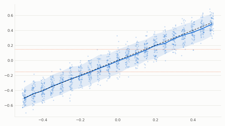
True φ on the horizontal axis, 1 − M²/2 from one 100-return window on the vertical. 400 simulated windows for each of 21 values of φ; dots show 60 of them, the band spans the 5th to 95th percentile, the solid line is the median, the dashed line is the identity. The dotted lines at ±0.15 are the classifier's two one-sided cut-offs: above for Trend, below for Revert.
The median tracks the identity with the small downward bias of short-window autocorrelations (at φ = 0.5 it is 0.480). At φ = 0 the 90% range runs from −0.18 to 0.15, so one window can read as trending with nothing there.
Rolling variances in constant time
Recomputing three 100-bar variances on every bar of history is wasteful. CRollingMoments keeps a running sum and sum of squares over a ring buffer:
//+------------------------------------------------------------------+
//| CRollingMoments::Push - add one value, evict the oldest          |
//+------------------------------------------------------------------+
void CRollingMoments::Push(const double x)
  {
//--- Window full: subtract the value about to be overwritten
   if(m_count==m_size)
     {
      double old=m_buf[m_head];
      m_sum  -=old;
      m_sumsq-=old*old;
     }
   else
      m_count++;
//--- Store the new value and advance the ring pointer
   m_buf[m_head]=x;
   m_sum  +=x;
   m_sumsq+=x*x;
   m_head=(m_head+1)%m_size;
//--- Periodic rebuild stops add/subtract rounding from accumulating
   m_since++;
   if(m_since>=m_every)
      Rebuild();
  }
Running sums drift with rounding, so every HJ_RECOMPUTE (1,000) pushes Rebuild() sums the buffer from scratch. CHjorthRolling wraps three of them and builds the differences on the fly:
//+------------------------------------------------------------------+
//| CHjorthRolling::Push - feed the next signal value                |
//+------------------------------------------------------------------+
void CHjorthRolling::Push(const double y)
  {
//--- The first difference exists from the second value onwards
   if(m_seen>=1)
     {
      double dy=y-m_prev_y;
      m_dy.Push(dy);
      //--- The second difference exists from the third value onwards
      if(m_seen>=2)
         m_d2y.Push(dy-m_prev_dy);
      m_prev_dy=dy;
     }
//--- The signal window always receives the value
   m_y.Push(y);
   m_prev_y=y;
   m_seen++;
  }
Once the Δ²y window holds N values, all three windows cover the same N bars. This matches the alignment used by the batch function HjorthCompute(). On 9,586 real XAUUSD H1 windows rolling and batch agree to 1.9e−14 (2.2e−14 without the rebuild, which guards much longer runs).
From three variances to the dashboard values
Both paths end in one function, so the formulas live in one place:
//+------------------------------------------------------------------+
//| Activity, Mobility, Complexity and rho1 from three variances     |
//+------------------------------------------------------------------+
bool HjorthFromVariances(const double var_y,
                         const double var_dy,
                         const double var_d2y,
                         SHjorthResult &out)
  {
   ZeroMemory(out);
//--- A flat window (zero variance) has no defined ratios
   if(var_y<=0.0 || var_dy<=0.0 || var_d2y<=0.0)
      return(false);
//--- Hjorth definitions
   double mobility   =MathSqrt(var_dy/var_y);        // M(y)
   double mobility_d =MathSqrt(var_d2y/var_dy);      // M(dy)
   out.activity  =var_y;
   out.mobility  =mobility;
   out.complexity=mobility_d/mobility;
//--- Var(dy) = 2*Var(y)*(1-rho1)  =>  rho1 = 1 - M^2/2
   out.rho1 =MathMax(-1.0,MathMin(1.0,1.0-0.5*mobility*mobility));
   out.valid=true;
   return(true);
  }
Two failure modes are handled here. A window with zero variance, such as a frozen feed, returns false and the bar stays empty. Sampling noise can push M past 2, which would put ρ₁ below −1, so the result is clamped. On the 9,688 exported XAUUSD H1 bars neither occurred: no window was flat and M stayed between 1.09 and 1.87. For the forming bar, HjorthFromCloses() converts N + 3 closes into N + 2 log returns. Both paths treat close ≤ 0 as a flat bar (returning 0) to keep bar indices aligned. That can hide a feed defect, biasing the window toward Quiet. Here it never fired: 0 of the 9,688 exported closes are ≤ 0, and the 5 zero returns in the export are genuinely unchanged closes.
Null bands and the regime classifier
HjorthNullBands() builds the cut-offs from the iid standard error of ρ₁:
SE(ρ1) ≈ 1 / √N
band   = z / √N = 1.5 / √100 = 0.15      (Mobility 1.304 and 1.517)

Trend:   ρ1 >= +band    right tail, nominal 6.7%
Revert:  ρ1 <= -band    left tail,  nominal 6.7%
The 6.7% rates rest on a normal approximation. That assumption does not hold well here. Simulating this estimator on iid returns gives 5.3% above +0.15, because of its negative bias. With GARCH-style volatility clustering it gives 7.1%. The test results below include a sensitivity check on the band.
Activity and Complexity are ranked against their own previous 500 values. HjorthPercentRank() counts ties as half and returns no rank until at least 250 values exist. Then the classifier checks the labels in order:
//+------------------------------------------------------------------+
//| Map one Hjorth reading and its percentiles to a regime label     |
//+------------------------------------------------------------------+
ENUM_HJ_REGIME HjorthClassify(const SHjorthResult &res,
                              const double act_pct,
                              const double cpx_pct,
                              const double rho_band,
                              const double quiet_pct,
                              const double shock_pct)
  {
//--- No reading or no percentile history yet
   if(!res.valid || act_pct<0.0 || cpx_pct<0.0)
      return(HJ_REGIME_NEUTRAL);
//--- Shape overrides everything: an irregular path is not a clean trend
   if(cpx_pct>=shock_pct)
      return(HJ_REGIME_SHOCK);
//--- Too little movement to be worth trading
   if(act_pct<=quiet_pct)
      return(HJ_REGIME_QUIET);
//--- Autocorrelation outside the null band decides direction of memory
   if(res.rho1>=rho_band)
      return(HJ_REGIME_TREND);
   if(res.rho1<=-rho_band)
      return(HJ_REGIME_REVERT);
   return(HJ_REGIME_NEUTRAL);
  }
Taken literally, a bar is Trend only if the Complexity percentile is below 0.90, the Activity percentile is above 0.20, and ρ₁ ≥ +0.15. Shock comes first because a jagged, gap-driven path is not a clean trend. That ordering is a design choice, and it is tested below.
"Trend" is a label for persistent returns, meaning positive lag-1 autocorrelation over the last 100 bars. It is not a directional price trend. A window can drift sideways with ρ₁ > 0, and the label carries no direction, so the gate never checks whether a breakout points the same way as recent returns. Every result below about "Trend breakouts" means breakouts taken in this positive-autocorrelation regime.
The dashboard indicator
HjorthParameters draws implied ρ₁ as a histogram colored by regime and two lines, with level lines at ±band and zero. Buffer 9 carries the regime number for iCustom().
Activity score    = 2 · ActivityPercentile - 1
Complexity excess = C / √1.5 - 1
//+------------------------------------------------------------------+
//| Custom indicator iteration function                              |
//+------------------------------------------------------------------+
int OnCalculate(const int rates_total,
                const int prev_calculated,
                const datetime &time[],
                const double &open[],
                const double &high[],
                const double &low[],
                const double &close[],
                const long &tick_volume[],
                const long &volume[],
                const int &spread[])
  {
//--- Window of returns, two lookback returns for the differences, one forming bar
   if(rates_total<InpWindow+4)
      return(0);
//--- First call, or history was rebuilt: start the rolling state from bar 1
   if(prev_calculated==0)
     {
      ClearBuffers();
      g_roll.Reset();
      g_last_fed=0;
     }
//--- Closed bars: push each new log return once, O(1) per bar
   int last_closed=rates_total-2;
   for(int i=g_last_fed+1;i<=last_closed;i++)
     {
      //--- A missing close is treated as a flat bar so indices stay aligned
      double r=(close[i]>0.0 && close[i-1]>0.0) ? MathLog(close[i]/close[i-1]) : 0.0;
      g_roll.Push(r);
      SHjorthResult res;
      g_roll.Result(res);
      WriteBar(i,res);
      g_last_fed=i;
     }
//--- Forming bar: batch recompute on every tick, never pushed into g_roll
   SHjorthResult live;
   HjorthFromCloses(close,rates_total-1,InpWindow,live);
   WriteBar(rates_total-1,live);
   return(rates_total);
  }
Closed bars go through the rolling state once each. The forming bar is recomputed from closes on every tick and never touches g_roll, which would otherwise receive the same bar again on every tick. WriteBar() stores the raw values, ranks them against earlier bars only, and classifies. The regime buffer stays EMPTY_VALUE until both ranks exist, and on XAUUSD H1 that is the first 352 bars.
The loop depends on bar order. Nothing calls ArraySetAsSeries(), so close[] and every buffer keep the default order: index 0 is the oldest bar and rates_total − 1 the forming one. Hence closed bars run from g_last_fed + 1 to rates_total − 2 and returns use close[i-1]. The EA reads via CopyBuffer(handle, buffer, 1, 1,...). The start position is counted back from the current bar, so position 1 always refers to the last closed bar.
Fig. 2. Hjorth dashboard on XAUUSD H1, 2 to 30 March 2026
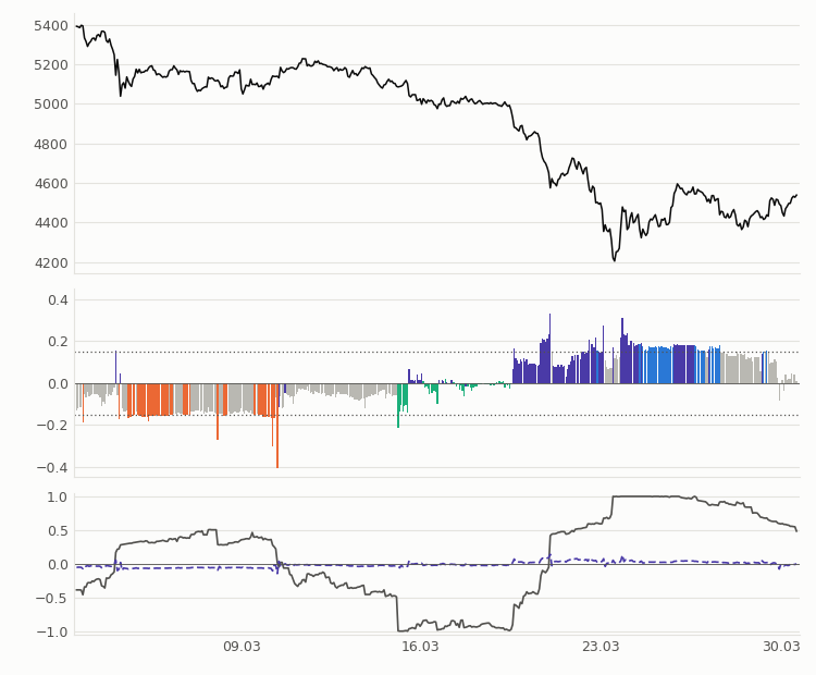
460 H1 bars. Top: close. Middle: implied ρ₁ colored by regime: gray Neutral, blue Trend, orange Revert, aqua Quiet, violet Shock; dotted lines are the two one-sided cut-offs at ±0.15. Bottom: Activity score (solid gray) and Complexity excess (dashed violet). Recomputed from the terminal's exported bars with the same formulas.
After the 3 March drop many bars are orange. From 13 to 17 March Activity sank and the bars turn aqua. During the fall to about 4,200 Complexity sat in its top tail, so the decline is mostly violet Shock, and the first run of blue Trend bars appears on 24 March. This single window illustrates the mechanism; it proves nothing about the full sample.
Checking the math
The EA runs HjorthRunSelfTest() in OnInit() and refuses to start if any of its 24 checks fails. They cover a pure sine (M = 2·sin(π/20) and C = 1 exactly), seeded white noise and AR(1) series against a Python mirror to 1e-9, rolling against batch results, the band constants, a tied percentile rank and every classifier branch.
All 24 passed in the terminal. The self-test does not cover the indicator's incremental OnCalculate() path, the close-to-return conversion, ranks over partly empty history, or any EA logic: signals, sizing, logging. To cover the indicator chain, I recomputed the dashboard from exported XAUUSD H1 bars and compared it with the EA's logged snapshots. Of 343 trades, 317 occur after the 603-bar warm-up required to build a full 500-bar rank history in the export. 314 of these match the logged regime, with a median ρ₁ difference of 2.5e−05, the CSV's rounding. The three mismatches all fall in July 2025. The first differs in ρ₁ and the other two only in rank, which is consistent with one bar that differs between the tester and the export. The EA logs nothing on other bars, so this checks 317 bars on one symbol, not every bar or both timeframes. These checks show that the code computes the formulas as written. They say nothing about whether the regimes are stable or useful as filters; that is what the tests below look at.
The regime-gated Expert Advisor
The EA trades a 20-bar Donchian breakout on the close of bar 1, with a stop at 2 × ATR(14), a target at 2R and 0.5% of equity at risk. InpUseGate changes one line:
//+------------------------------------------------------------------+
//| Expert tick function                                             |
//+------------------------------------------------------------------+
void OnTick()
  {
//--- Decisions are made once per closed bar of the working timeframe
   if(!IsNewBar())
      return;
//--- One position at a time for this symbol and magic
   if(HasOpenPosition())
      return;
//--- Breakout direction from the bar that just closed
   int direction=DonchianSignal();
   if(direction==0)
      return;
//--- Dashboard reading for the same closed bar (gate OFF waits for it too)
   int    regime;
   double rho1,act_pct,cpx_pct;
   if(!ReadDashboard(regime,rho1,act_pct,cpx_pct))
      return;
//--- The gate: with the filter on, only the Trend regime may trade
   if(InpUseGate && regime!=HJ_REGIME_TREND)
      return;
   OpenTrade(direction,regime,rho1,act_pct,cpx_pct);
  }
With the gate off, the EA still waits for the dashboard, so every gate-OFF trade carries a regime label. The gate uses only the right-tail label. The reading comes through iCustom() from closed bar 1, the bar the breakout is measured on:
//+------------------------------------------------------------------+ //| Read regime, rho1 and both percentiles for closed bar 1 | //+------------------------------------------------------------------+ bool ReadDashboard(int ®ime,double &rho1,double &act_pct,double &cpx_pct) { regime =HJ_REGIME_NEUTRAL; rho1 =0.0; act_pct=-1.0; cpx_pct=-1.0; //--- The indicator must have caught up with history if(BarsCalculated(g_hj_handle)<InpHjWindow+4) return(false); //--- Buffers: 0 rho1, 7 Activity pct, 8 Complexity pct, 9 regime double b_rho[1],b_act[1],b_cpx[1],b_reg[1]; if(CopyBuffer(g_hj_handle,0,1,1,b_rho)!=1 || CopyBuffer(g_hj_handle,7,1,1,b_act)!=1 || CopyBuffer(g_hj_handle,8,1,1,b_cpx)!=1 || CopyBuffer(g_hj_handle,9,1,1,b_reg)!=1) return(false); //--- EMPTY_VALUE means the percentile history is still too short if(b_reg[0]==EMPTY_VALUE || b_rho[0]==EMPTY_VALUE) return(false); regime =(int)MathRound(b_reg[0]); rho1 =b_rho[0]; act_pct=b_act[0]; cpx_pct=b_cpx[0]; return(true); }
Each closed trade is scored in R. CalcLots() computes the money at risk from the planned stop distance before the order is sent; OpenTrade() stores it in an entry snapshot, and OnTradeTransaction() matches the closing deal to that snapshot by position id:
loss_per_lot = stop_distance / tick_size · tick_value
               (stop_distance · contract_size if they differ over 3x)
risk_money   = lots · loss_per_lot
R            = (profit + swap + entry and exit commission) / risk_money
On 5,375 logged trades that denominator matches lots × |fill − stop| × contract size (100 for gold, 100,000 for FX) within 0.6% for 99% of trades and 5.3% at most. The gap is slippage between the requested price and the fill; the largest is a EURUSD M15 entry at the Monday open on 2025.01.27. Each run truncates its own CSV at start.
Strategy Tester results
Settings: MetaQuotes-Demo, every tick based on real ticks, 2025.01.01 to 2026.08.31, $10,000, 1:100, a 5 ms delay, default inputs, and 100% history quality on all three symbols. Each symbol ran on H1 and M15, once with the gate and once without.
Sample accounting. The 5,119 gate-OFF trades and 256 gate-ON trades are every closed trade in the twelve CSVs, and every statistic below uses them, so it can be rebuilt from the attached files. A CSV is one trade short of the tester report when the tester force-closes a final position after the EA stops receiving events. Where I have the report: XAUUSD H1 344 against 343 trades ($692.13 against $626.32), EURUSD H1 354 against 353 (−$869.06 against −$941.30), GBPUSD H1 379 against 379 ($239.07 both).
Tests. Means are tested against zero with two-sided t-tests, intervals are two-sided 95% Student-t, and two groups are compared with a two-sided Welch test. These tests treat trades as independent, which is not true. Trades on the same days share news, and EURUSD and GBPUSD are correlated. The t-test p-values and intervals are therefore optimistic, so the regime table adds a p-value from resampling whole calendar weeks. Gate-ON legs under 30 trades (XAUUSD H1, EURUSD H1, GBPUSD H1: 4, 23 and 18) are listed but not interpreted.
| Leg | Gate | Trades | Win % | Mean R | 95% CI | p | Net, $ | Max DD % |
|---|---|---|---|---|---|---|---|---|
| XAUUSD H1 | OFF | 343 | 35.3 | +0.041 | ±0.156 | 0.603 | +626 | 7.4 |
| XAUUSD H1 | ON | 4 | 25.0 | −0.252 | ±2.406 | 0.761 | −15 | 0.7 |
| XAUUSD M15 | OFF | 1,405 | 34.8 | +0.031 | ±0.077 | 0.423 | +1,843 | 17.7 |
| XAUUSD M15 | ON | 78 | 26.9 | −0.203 | ±0.305 | 0.188 | −486 | 9.3 |
| EURUSD H1 | OFF | 353 | 32.0 | −0.052 | ±0.148 | 0.494 | −941 | 14.7 |
| EURUSD H1 | ON | 23 | 43.5 | +0.297 | ±0.660 | 0.360 | +322 | 2.0 |
| EURUSD M15 | OFF | 1,328 | 30.7 | −0.097 | ±0.076 | 0.013 | −4,849 | 53.0 |
| EURUSD M15 | ON | 55 | 18.2 | −0.463 | ±0.319 | 0.005 | −1,181 | 11.8 |
| GBPUSD H1 | OFF | 379 | 34.3 | +0.017 | ±0.146 | 0.817 | +239 | 8.8 |
| GBPUSD H1 | ON | 18 | 38.9 | +0.160 | ±0.751 | 0.659 | +147 | 3.8 |
| GBPUSD M15 | OFF | 1,311 | 28.7 | −0.170 | ±0.076 | <0.001 | −6,735 | 69.5 |
| GBPUSD M15 | ON | 78 | 21.8 | −0.354 | ±0.284 | 0.015 | −1,274 | 14.0 |
The gate removes 93.5% to 98.8% of trades, so dollar results mostly measure exposure. Mean R takes out the money scale. It does not take out the change in which trades are taken. Of the 256 gate-ON trades, 179 are the same entries the ungated EA took, same bar and same direction, with R identical to within 0.0009, and all 179 are labeled Trend there. The other 77 exist only because the gated EA was flat on bars where the ungated one was still in a position. The shared trades average −0.252R (p = 0.011), the other 77 −0.196R (p = 0.210). Therefore, the ON-versus-OFF difference conflates the filter effect with position occupancy, entry order, and missed signals. It is not a clean estimate of the filter. Without the gate, only EURUSD M15 and GBPUSD M15 differ significantly from zero, and both lose (p = 0.013 and p < 0.001). Pooled, gate-ON trades average −0.235R (95% CI ±0.163, p = 0.005).
The cleaner test of the label stays inside the gate-OFF runs: the same trades on the same bars, split by the regime logged at entry. It still inherits the ungated system's occupancy, so it describes the label on the trades that system was free to take:
| Regime at entry | Trades | Share | Win % | Mean R | 95% CI | p | Week-cluster p |
|---|---|---|---|---|---|---|---|
| Neutral | 2,512 | 49.1% | 32.5 | −0.047 | ±0.057 | 0.106 | 0.184 |
| Trend | 187 | 3.7% | 25.1 | −0.252 | ±0.189 | 0.009 | 0.013 |
| Revert | 413 | 8.1% | 31.0 | −0.078 | ±0.136 | 0.263 | 0.277 |
| Quiet | 955 | 18.7% | 32.7 | −0.047 | ±0.093 | 0.320 | 0.330 |
| Shock | 1,052 | 20.6% | 31.7 | −0.061 | ±0.085 | 0.165 | 0.300 |
Fig. 3. Mean R of gate-OFF breakouts by regime at entry, six legs pooled
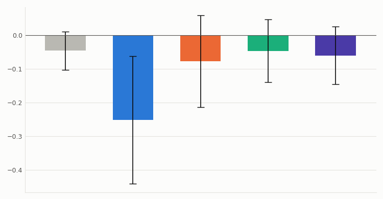
Left to right: Neutral (gray), Trend (blue), Revert (orange), Quiet (aqua), Shock (violet), 5,119 trades. Whiskers are two-sided 95% Student-t intervals; values are in the table above.
Breakouts in the Trend regime did worst, and theirs is the only t-interval that excludes zero. Its week-cluster p is 0.013. Against all other breakouts the difference is −0.20R (Welch p = 0.043), and resampling whole calendar weeks (87 weeks, 10,000 draws) puts it between −0.41 and −0.003R (p = 0.047).
Gaps don't drive the Trend result. 122 gate-OFF trades fall outside −1.2R to +2.2R (47 at the Monday open, 42 at the session open, 20 at 15:30 server time, 13 elsewhere; the worst closed at −8.4R). Without them the Trend difference is −0.23R (p = 0.023).
Relabeling the logged snapshots reproduces the EA's own label on 5,119 of 5,119 trades, so other bands and an order with Trend checked before Shock and Quiet can be applied to the same trades. This tests how stable the label is. It does not re-run the EA, so the trades taken and the position occupancy stay those of the shipped settings:
| z | Band | Order | Trend trades | Mean R | 95% CI | p |
|---|---|---|---|---|---|---|
| 1.0 | 0.10 | Shock, Quiet, then ρ₁ (shipped) | 404 | −0.192 | ±0.133 | 0.005 |
| 1.0 | 0.10 | ρ₁ first | 930 | −0.148 | ±0.089 | 0.001 |
| 1.5 | 0.15 | Shock, Quiet, then ρ₁ (shipped) | 187 | −0.252 | ±0.189 | 0.009 |
| 1.5 | 0.15 | ρ₁ first | 547 | −0.126 | ±0.116 | 0.033 |
| 2.0 | 0.20 | Shock, Quiet, then ρ₁ (shipped) | 92 | −0.189 | ±0.280 | 0.182 |
| 2.0 | 0.20 | ρ₁ first | 287 | −0.172 | ±0.158 | 0.032 |
Trend-labeled breakouts are negative in all six variants, and their t-interval excludes zero in five. These post-hoc checks on the same data show that the label is stable under nearby settings, not that the trading system is. Several factors can produce the pattern together. The 100-bar ρ₁ responds late, the ordering moves early persistent bars into Shock, the label ignores breakout direction, the band fires more often than its nominal rate (at breakout bars 12.2% of readings are above +0.15), and the samples are small. These tests do not separate those factors.
The article reports 34 p-values: 12 legs, 5 regimes with two each, 3 Trend-versus-rest comparisons, 3 gate-ON means and 6 relabeling variants. Under a Holm correction across all 34, the Trend regime's t-test gives an adjusted p of 0.27 and its week-cluster test 0.33. Only two results survive: GBPUSD M15 gate OFF losing money, and one post-hoc relabeling variant. The Trend finding is a direction to test on fresh data. It is not an established effect.
Fig. 4. Mean R per leg, gate OFF and ON
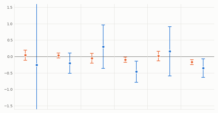
Left to right: XAUUSD H1, XAUUSD M15, EURUSD H1, EURUSD M15, GBPUSD H1, GBPUSD M15. Orange gate OFF, blue gate ON, with two-sided 95% Student-t intervals. The axis stops at ±1.6; the XAUUSD H1 gate-ON interval (4 trades) is ±2.41 and is cut off.
Limitations
Scope. One broker (MetaQuotes-Demo), one period (2025.01.01 to 2026.08.31), three instruments, two timeframes and one strategy: a 20-bar Donchian breakout with a 2 × ATR stop, a 2R target and default inputs.
Design set in advance. z = 1.5, N = 100 and the ordering were set before the runs.
Approximations. The band assumes iid returns. The t-tests assume independent trades with near-normal means, which calendar overlap and correlated pairs violate; the week-cluster p-values are the more honest guide. Samples of 4 to 78 gate-ON trades are too small for stable conclusions per leg.
Sizing. On XAUUSD H1, 52.5% of trades used 0.01 lot (average risk $40.59 against $50); R uses each trade's actual risk. Signals skipped because the minimum lot exceeded the budget go only to the Journal, so they are not counted.
Conclusion
Hjorth's parameters give volatility, lag-1 autocorrelation and path shape from one calculation over three variances, and ρ₁ = 1 − M²/2 makes Mobility readable. The self-test and the replay from exported bars show that the code computes them as specified, not that the regimes are stable or useful as filters.
As a breakout filter in these tests, gating on the positive-autocorrelation (Trend) regime did not help. Breakouts taken in that regime had the lowest mean R of the five groups, the pattern held across six relabeling variants, and gate-ON trades lost on average. After a correction across all 34 reported tests, though, none of the Trend results is significant, so this is a suggestive pattern, not proof of harm. All of this applies to XAUUSD, EURUSD and GBPUSD on H1 and M15, MetaQuotes-Demo, 2025 to 2026, with this breakout and these exits. The Revert and Quiet labels were not tested as filters.
| File | Type | Description |
|---|---|---|
| MQL5\Include\HjorthDashboard\HjorthCore.mqh | Include | Rolling moments, Hjorth calculation, null bands, percentile rank, classifier, CSV helper, 24-check self-test. |
| MQL5\Indicators\HjorthDashboard\HjorthParameters.mq5 | Indicator | Regime-colored ρ₁ histogram, Activity score and Complexity excess; regime in buffer 9. |
| MQL5\Experts\HjorthDashboard\HjorthRegime_EA.mq5 | Expert Advisor | Donchian breakout with an optional Trend gate; one CSV row per closed trade and a per-regime summary. |
| MQL5\Files\HjorthDashboard\*.py | Python | Reference implementation, replay from exported bars, statistics and figures. |
Warning: All rights to these materials are reserved by MetaQuotes Ltd. Copying or reprinting of these materials in whole or in part is prohibited.
This article was written by a user of the site and reflects their personal views. MetaQuotes Ltd is not responsible for the accuracy of the information presented, nor for any consequences resulting from the use of the solutions, strategies or recommendations described.


