Developing Statistical Market Inflection Forecasting Indicator
 122
 0

Table of Contents
- Introduction
- System Overview
- Getting Started
- Enumerations and Inputs
- Data Structures
- The Statistical Helper
- Loading History and Replaying it in Order
- The Per-Bar Pipeline
- Detecting References
- Tracking the Movement and Its Termination
- Turning a Movement into an Observation
- Features and Higher-Timeframe Context
- Snapshot: One Decision per Reference
- Selecting Similar Historical Movements
- From Distribution to Entry, Stop, and Target
- Empirical Hit Rates by Replay
- The Replay Rules
- The Forecast State Machine
- Rendering Active Forecasts and Removing Resolved Ones
- The Previous-Forecast Layer
- The Dashboard
- CSV Export and the Main Handler
- Indicator Demo
- Limitations and Proper Use
- Conclusion
Introduction
Most discretionary reversal traders face the same problem. They see a strong move, and they know it will end somewhere. The question is where. Often they reach for a round number, a fixed pip target, or a Fibonacci level they read about years ago. The stop goes a "comfortable" distance away. These levels can work, but they are rarely checked against how the instrument in front of them has actually behaved.
The tools do not help much either. Many reversal indicators repaint, so the arrow that looked perfect in hindsight was never there in real time. Others print a confidence value, such as "82% probability", without saying how it was measured or on how many cases. A trader cannot tell whether that number comes from a thousand past events or from nothing at all. This is point A: decisions about the turning point, the stop and the target are often made on assumptions that were not tested on the market in front of us.
In this article, we build a different kind of tool. It does not replace structure-based stops, volatility-scaled targets or other valid methods. It adds one more input: levels measured on the history of the symbol we trade. We develop the Statistical Market Inflection Forecasting indicator (SMIF). It does not claim that price will reverse. It says something more modest and more useful: similar historical movements ended at these distances. They moved this far in the opposite direction and hit these levels with this frequency. Entry, stop and take profit are read from those distributions (unless an optional fallback stop is enabled). The hit rates come from a chronological replay that only uses bars that were already closed at each decision. These are historical frequencies, not guarantees. A level built from past distributions helps only if the market continues to behave similarly. We discuss cases where this assumption fails before the conclusion. When a forecast resolves, its objects leave the chart, and a single toggle brings them back for review.
System Overview
The indicator works on one analysis timeframe, which can be the chart timeframe or any timeframe from M1 to D1. It first detects confirmed reference points. A reference high is a local high confirmed by a number of bars on each side; price is then expected to move down from it. A reference low is the mirror case. After confirmation, the indicator tracks the movement that develops from the reference. When that movement has travelled a minimum distance, measured in ATR, the indicator takes a single "snapshot". At that bar it records a feature vector: distance, duration, volatility, momentum, acceleration, candle body statistics, retracement depth, the share of directional candles, time of day and the position relative to a higher-timeframe EMA.
The movement is then followed until it terminates. Termination has a formal, rule-based definition: price must retrace from the extreme by a threshold that combines ATR and a fraction of the leg. After termination, the indicator follows the opposite move until that move also terminates, or until price resumes past the original extreme. Only then does the movement become a completed historical observation. Each observation stores, in ATR units, how much further price extended after the snapshot and how far the opposite move reached. This database is the only source of statistics. Nothing about how far price "should" move is hard-coded. The rules, thresholds and percentiles, however, are parameters that we choose. They make the method repeatable, but they do not by themselves prove that it has an edge.
When a snapshot is taken, the forecasting engine selects the most similar completed observations. From the remaining-extension distribution it takes a percentile, which becomes the predicted termination and the suggested entry. The adverse excursion beyond that entry gives the stop. The opposite-move distribution gives the take profit. The engine then replays these levels on historical bars. For each neighbor, it scales the levels and counts how often price reaches the entry, stop, or target. The forecast is shown only if these empirical numbers pass the filters. Note that these counts come from the same neighbors that were used to derive the levels, so they are an in-sample measure. The forward results of forecasts tracked after their creation, shown in the validation section of the dashboard, are the more honest measure. A state machine then tracks the forecast bar by bar until it reaches TP, reaches SL, is invalidated or expires.
| State | Meaning |
|---|---|
| NO_FORECAST | No developing reference and no open forecast |
| REFERENCE_DETECTED | A reference was confirmed on this bar |
| MOVEMENT_DEVELOPING | The movement from the reference is being tracked |
| FORECAST_READY | A forecast exists and waits for price to reach the entry (developing forecast) |
| ENTRY_REACHED | The entry was touched on this bar |
| FORECAST_ACTIVE | The entry was filled and the forecast is running (confirmed forecast) |
| TP_REACHED | The statistical target was reached (resolved) |
| SL_REACHED | The statistical stop was violated (resolved) |
| FORECAST_INVALIDATED | The reference broke, the target came before the entry, the entry expired, or the holding time ran out (resolved) |
Getting Started
Enumerations and Inputs
//+------------------------------------------------------------------+
//|                                                         SMIF.mq5 |
//|                                  Copyright 2025, MetaQuotes Ltd. |
//|                     https://www.mql5.com/en/users/johnhlomohang/ |
//+------------------------------------------------------------------+
#property copyright "Copyright 2025, MetaQuotes Ltd."
#property link      "https://www.mql5.com/en/users/johnhlomohang/"
#property version   "1.00"
#property indicator_chart_window
#property indicator_buffers 0
#property indicator_plots   0

//--- every object created by this indicator starts with SMIF_
#define SMIF_PREFIX       "SMIF_"
#define SMIF_PREV_PREFIX  "SMIF_PREV_"
#define SMIF_DASH_PREFIX  "SMIF_DASHBOARD_"
#define SMIF_BTN_PREV     "SMIF_BTN_PREV"
//--- number of similarity features
#define SMIF_FEAT         12

//+------------------------------------------------------------------+
//| Enumerations                                                     |
//+------------------------------------------------------------------+
enum ENUM_SMIF_TIMEFRAME
  {
   SMIF_TF_CURRENT=0,   // Current Chart
   SMIF_TF_M1,          // M1
   SMIF_TF_M5,          // M5
   SMIF_TF_M15,         // M15
   SMIF_TF_M30,         // M30
   SMIF_TF_H1,          // H1
   SMIF_TF_H4,          // H4
   SMIF_TF_D1           // D1
  };

enum ENUM_REFERENCE_TYPE
  {
   REFERENCE_HIGH=0,    // Reference high (movement develops downward)
   REFERENCE_LOW=1      // Reference low (movement develops upward)
  };

enum ENUM_FORECAST_DIRECTION
  {
   FORECAST_SELL=-1,
   FORECAST_NONE=0,
   FORECAST_BUY=1
  };

enum ENUM_FORECAST_STATE
  {
   STATE_NO_FORECAST=0,
   STATE_REFERENCE_DETECTED,
   STATE_MOVEMENT_DEVELOPING,
   STATE_FORECAST_READY,
   STATE_ENTRY_REACHED,
   STATE_FORECAST_ACTIVE,
   STATE_TP_REACHED,
   STATE_SL_REACHED,
   STATE_FORECAST_INVALIDATED
  };

enum ENUM_FORECAST_OUTCOME
  {
   OUTCOME_NONE=0,
   OUTCOME_TP,
   OUTCOME_SL,
   OUTCOME_INVALIDATED,
   OUTCOME_EXPIRED
  };
We begin with the enumerations that describe the life of a forecast. The state enumeration mirrors the table above one to one, so every value we see on the dashboard or in the log maps directly to a stage in the lifecycle. The outcome enumeration is kept separate from the state because the two answer different questions. The state tells us where a forecast is right now, while the outcome records how it finished. A forecast that expired after entry, for example, ends in the invalidated state but keeps the EXPIRED outcome, so validation statistics can still separate it from a forecast that never reached its entry.
//+------------------------------------------------------------------+
//| Inputs                                                           |
//+------------------------------------------------------------------+
input group "=== Analysis ==="
input ENUM_SMIF_TIMEFRAME InpAnalysisTimeframe = SMIF_TF_CURRENT; // Analysis timeframe
input int      InpHistoryBars              = 10000;  // Closed bars loaded for the statistical database
input int      InpATRPeriod                = 14;     // ATR period (Wilder)

input group "=== Reference Detection ==="
input int      InpReferenceLeftBars        = 5;      // Left confirmation bars
input int      InpReferenceRightBars       = 3;      // Right confirmation bars
input double   InpMinimumMoveATR           = 1.0;    // Minimum move from reference (ATR) to qualify
input int      InpMinimumPriceDistance     = 0;      // Minimum move from reference (points)
input int      InpMaximumReferenceAge      = 60;     // Max bars for a reference to qualify

input group "=== Movement Termination ==="
input double   InpTerminationATR           = 1.0;    // Retracement needed to confirm termination (ATR)
input double   InpTerminationRetracement   = 0.382;  // Retracement needed (fraction of the leg)
input double   InpMinimumOppositeMove      = 0.5;    // Minimum opposite move (ATR)
input bool     InpRequireConfirmation      = true;   // Require a CLOSE beyond the threshold
input int      InpMaxObservationBars       = 300;    // Max bars a historical observation may span

input group "=== Statistical Engine ==="
input int      InpMinimumHistoricalSamples = 40;     // Minimum comparable observations in the pool
input int      InpSimilaritySamples        = 80;     // Nearest observations used (K)
input double   InpTerminationPercentile    = 40.0;   // Termination percentile (entry depth)
input double   InpStopPercentile           = 80.0;   // Adverse-excursion percentile (stop)
input double   InpTargetPercentile         = 45.0;   // Opposite-move percentile (target)
input double   InpStopBufferATR            = 0.10;   // Buffer beyond the statistical stop (ATR)
input bool     InpUseFallbackSL            = false;  // Use fixed fallback SL when samples are thin
input double   InpFallbackSLATR            = 1.5;    // Fallback SL (ATR)
input bool     InpUseSessionFeature        = true;   // Use time-of-day in similarity
input bool     InpUseContextFeature        = true;   // Use higher-timeframe context in similarity
input ENUM_TIMEFRAMES InpContextTimeframe  = PERIOD_H4; // Higher timeframe for context
input int      InpContextEMAPeriod         = 50;     // Higher-timeframe EMA period

input group "=== Forecast Filters ==="
input int      InpMinimumSamples           = 20;     // Minimum filled samples
input double   InpMinimumTPHitRate         = 40.0;   // Minimum TP hit rate (%)
input double   InpMaximumSLHitRate         = 55.0;   // Maximum SL hit rate (%)
input double   InpMinimumRiskReward        = 0.8;    // Minimum reward:risk
input double   InpMinimumExpectedMovePercent = 0.05; // Minimum expected move (%)
input bool     InpSingleOpenForecast       = true;   // One open forecast per direction
The inputs are grouped by responsibility. The reference detection group controls how strict the pivots are and how far a movement must travel, in ATR and in points, before it qualifies. The termination group defines when a movement is considered finished. We combine an ATR threshold, a fraction of the leg and a minimum opposite move, and we optionally require a candle close beyond the threshold rather than a wick. The statistical group sets the pool size, the number of nearest neighbors and the three percentiles that turn distributions into prices. The filter group decides when a forecast is strong enough to be displayed at all. Two sample inputs are easy to confuse. InpMinimumHistoricalSamples is the minimum number of comparable observations in the candidate pool before any forecast is evaluated. InpMinimumSamples is the minimum number of neighbors whose replayed trade actually reached the entry. The first protects the similarity search, the second protects the hit rates. The defaults of 40 and 20 are working minimums, not statistically comfortable sample sizes. The fallback stop, InpUseFallbackSL, is off by default because it replaces the statistical stop with a fixed ATR multiple.
input group "=== Forecast Lifecycle ==="
input int      InpForecastExpiryBars       = 30;     // Bars to reach entry before invalidation
input int      InpMaxHoldBars              = 120;    // Bars after entry before expiry
input bool     InpValidationMode           = true;   // Generate & resolve forecasts on history

input group "=== Visualization ==="
input color    InpRiskColor                = clrCrimson;    // Risk rectangle colour
input color    InpRewardColor              = clrDodgerBlue; // Reward rectangle colour
input color    InpEntryColor               = clrGold;       // Entry line colour
input int      InpRectangleTransparency    = 65;     // Rectangle transparency (0-100)
input int      InpRectangleExtensionBars   = 20;     // Rectangle extension into future bars
input bool     InpShowLabels               = true;   // Show forecast labels
input int      InpLabelFontSize            = 8;      // Label font size

input group "=== Previous Forecasts ==="
input bool     InpShowPreviousForecasts    = false;  // Show previous forecasts at start (toggle: button or P)
input bool     InpPrevShowTP               = true;   // Previous: show TP reached
input bool     InpPrevShowSL               = true;   // Previous: show SL reached
input bool     InpPrevShowInvalidated      = true;   // Previous: show invalidated / expired
input int      InpMaxPreviousDrawn         = 150;    // Previous: maximum drawn
input int      InpPreviousTransparency     = 82;     // Previous: rectangle transparency (0-100)
The lifecycle group sets how long a forecast may wait for its entry and how long it may be held after entry. The validation mode switch decides whether forecasts are also generated and resolved on history. The previous forecasts group controls the layer that shows resolved forecasts, whether that layer is visible at start, which outcomes it includes, how many it draws and how faded it looks.
Data Structures
//+------------------------------------------------------------------+
//| Structures                                                       |
//+------------------------------------------------------------------+
struct SReference
  {
   long              id;
   int               type;            // ENUM_REFERENCE_TYPE
   int               dirMove;         // -1 movement down (from a high), +1 movement up (from a low)
   double            price;
   datetime          time;
   int               bar;             // chronological bar index of the reference
   int               confirmBar;      // bar at which it became confirmed
   int               phase;           // 0 developing, 1 opposite leg, 2 finished, 3 dropped
   double            extreme;
   int               extremeBar;
   double            oppPeak;
   int               oppPeakBar;
   int               termConfirmBar;
   bool              snapshotTaken;
   int               snapBar;
   double            snapClose;
   double            snapATR;
   double            feat[SMIF_FEAT];
   bool              evaluated;
  };
The SReference structure holds everything we know about one reference and the movement growing from it. The field dirMove is the key to keeping both directions in one code path. It is -1 for a movement down from a high and +1 for a movement up from a low. Multiplying a price difference by dirMove turns it into "progress in the movement direction", so the same formula serves buys and sells. The phase field drives the tracking logic: developing, opposite leg, finished or dropped. The snapshot fields store the single decision moment, including the feature vector.
//--- completed historical movement = one statistical observation
struct SHistoricalObservation
  {
   long              refId;
   int               refType;
   double            refPrice;
   datetime          refTime;
   int               dirMove;
   double            initATR;
   double            initVol;
   double            initMom;
   int               snapBar;
   double            snapClose;
   double            snapATR;
   double            feat[SMIF_FEAT];
   double            maxExtension;
   double            termPrice;
   double            termDist;
   double            termPct;
   int               termDuration;
   double            oppDist;
   double            oppPct;
   int               oppDuration;
   double            mae;             // price extension beyond the snapshot (continuation)
   double            mfe;             // opposite excursion beyond the snapshot
   double            remN;            // remaining extension after the snapshot (ATR)
   double            favN;            // opposite peak relative to the snapshot close (ATR)
   int               completeBar;     // first bar at which this observation is known
   int               outcome;         // ENUM_OBS_OUTCOME
  };
The SHistoricalObservation structure is one row of the statistical database. Besides the descriptive fields required by the specification, two fields do most of the work. The field remN stores how far price extended after the snapshot, in ATR at the snapshot. The field favN stores how far the opposite move reached, measured from the snapshot close in the same unit. Normalizing by ATR makes observations from quiet and volatile periods comparable in scale. It does not make different market regimes, sessions or news periods equivalent, which is one reason the similarity search also uses volatility, time of day and higher-timeframe context. The field completeBar is the first bar at which this observation could be known. It is our main guard against look-ahead.
The Statistical Helper
//+------------------------------------------------------------------+
//| CStats - descriptive statistics                                  |
//+------------------------------------------------------------------+
class CStats
  {
public:
   //--- linear-interpolated percentile (0..100)
   static double     Percentile(const double &src[],const double pct)
     {
      int n=ArraySize(src);
      if(n<=0)
         return 0.0;
      double tmp[];
      ArrayCopy(tmp,src);
      ArraySort(tmp);
      if(n==1)
         return tmp[0];
      double p  =MathMax(0.0,MathMin(100.0,pct));
      double pos=p/100.0*(n-1);
      int    lo =(int)MathFloor(pos);
      int    hi =(int)MathCeil(pos);
      return tmp[lo]+(tmp[hi]-tmp[lo])*(pos-lo);
     }
Every distribution in the system goes through the percentile function of the CStats class. It copies and sorts the sample, then interpolates linearly between the two nearest ranks. Linear interpolation matters with small samples, because it avoids large jumps in the entry, stop or target when a single observation enters or leaves the neighborhood. The same class also provides the mean, the standard deviation and a descriptive summary with the 25th, 50th, 75th and 90th percentiles, which we print in debug mode.
Loading History and Replaying it in Order
   //+--------------------------------------------------------------+
   //| Initial load and historical replay                           |
   //+--------------------------------------------------------------+
   bool              Load(void)
     {
      m_ready=false;
      ArrayFree(m_rates);
      ArrayFree(m_atr);
      ArrayFree(m_refs);
      ArrayFree(m_obs);
      ArrayFree(m_fc);
      m_nextRefId=0;
      m_nextFcId=0;
      m_lastReject="";
      m_lastRejectTime=0;
      m_engineState=STATE_NO_FORECAST;
      ZeroMemory(m_move);

      int warm =WarmupBars();
      int avail=Bars(m_symbol,m_tf);
      if(avail<warm+100)
         return false;
      int count=(InpHistoryBars<avail-1) ? InpHistoryBars : avail-1;
      ResetLastError();
      int got=CopyRates(m_symbol,m_tf,1,count,m_rates);
      if(got<warm+100)
        {
         ArrayFree(m_rates);
         return false;
        }
      m_lastBar=got-1;
      ArrayResize(m_atr,got,1000);
      for(int i=0;i<got;i++)
         ComputeATR(i);
      if(!LoadContext())
        {
         ArrayFree(m_rates);
         ArrayFree(m_atr);
         return false;
        }
      //--- chronological replay: the same code path used live
      m_inHistory=true;
      m_liveStart=InpValidationMode ? warm : IMax(warm,m_lastBar-InpForecastExpiryBars);
      for(int i=warm;i<=m_lastBar;i++)
         ProcessBar(i);
      m_inHistory=false;
      m_ready=true;
      PrintFormat("[SMIF] %s %s ready: %d bars, %d observations, %d forecasts",
                  m_symbol,TFToString(m_tf),got,ArraySize(m_obs),ArraySize(m_fc));
      return true;
     }
The Load method copies closed bars of the analysis timeframe, starting from index 1 so the forming bar is never included. It computes Wilder's ATR on those bars internally, rather than through an indicator handle, so the values are deterministic on any timeframe. It then loads the higher-timeframe context and replays every bar from the warm-up point forward through ProcessBar. When validation mode is off, forecasts are only allowed near the end of history, so the current forecast still appears when the indicator is attached, while the database is still built from the full history.
   //--- appends newly closed bars and processes them one by one
   int               SyncNewBars(void)
     {
      if(!m_ready || m_lastBar<0)
         return 0;
      datetime lastClosed=iTime(m_symbol,m_tf,1);
      if(lastClosed==0 || lastClosed<=m_rates[m_lastBar].time)
         return 0;
      MqlRates tmp[];
      int got=CopyRates(m_symbol,m_tf,m_rates[m_lastBar].time,lastClosed,tmp);
      if(got<=0)
         return 0;
      if(m_ctxEnabled && iTime(m_symbol,InpContextTimeframe,0)!=m_ctxLastOpen)
         ReloadContext();
      int added=0;
      for(int k=0;k<got;k++)
        {
         if(tmp[k].time<=m_rates[m_lastBar].time)
            continue;
         int n=m_lastBar+1;
         ArrayResize(m_rates,n+1,1000);
         ArrayResize(m_atr,n+1,1000);
         m_rates[n]=tmp[k];
         m_lastBar=n;
         ComputeATR(n);
         ProcessBar(n);
         added++;
        }
      if(added>0)
         Log(StringFormat("New bar %s processed. Observations=%d",TimeToString(m_rates[m_lastBar].time),ArraySize(m_obs)));
      return added;
     }
SyncNewBars handles live operation. It asks for the time of the last closed bar and copies any bars that are newer than the last one already stored. Each new bar is appended, its ATR is computed and it goes through the same ProcessBar call used during the replay. Because the function only reacts to closed bars, a forecast state can never flicker within a bar. It also means the timer can call it safely when the chart timeframe differs from the analysis timeframe and ticks do not arrive in step with it.
The Per-Bar Pipeline
   //+-------------------------------------------------------------+
   //| per-bar pipeline                                            |
   //+-------------------------------------------------------------+
   void              ProcessBar(const int i)
     {
      DetectReferences(i);
      //--- pass 1: movement tracking and completion of observations
      int n=ArraySize(m_refs);
      for(int k=0;k<n;k++)
         TrackReference(m_refs[k],i);
      //--- pass 2: snapshots and forecast evaluation (database now contains everything known at i)
      for(int k=0;k<n;k++)
         if(m_refs[k].phase==0 && !m_refs[k].snapshotTaken && i>=m_refs[k].confirmBar)
            TrySnapshot(m_refs[k],i);
      UpdateForecasts(i);
      CompactReferences();
      UpdateMarketInfo(i);
     }
ProcessBar is short, but its order is deliberate. First, we detect new references. Then, in a first pass, we update every tracked movement, which may complete observations and add them to the database. Only after that, in a second pass, do we take snapshots and evaluate forecasts. This means a forecast at bar i can use every observation completed at or before bar i, and nothing after. This order is valid because ProcessBar only runs on a closed bar. Every decision is taken at the close of bar i. A forecast created there can only be filled from bar i+1 onward because Simulate starts checking from the next bar. If the same logic were run inside a forming bar, it would use the high, low and close of a bar that has not finished, which is look-ahead. Open forecasts are updated next, finished references are removed, and the market information for the dashboard is refreshed.
Detecting References
   //+-------------------------------------------------------------+
   //|  reference detection (confirmed pivots only, never repaints)|
   //+-------------------------------------------------------------+
   void              DetectReferences(const int i)
     {
      int lb=InpReferenceLeftBars;
      int rb=InpReferenceRightBars;
      int p =i-rb;
      if(p-lb<0)
         return;
      bool isHigh=true,isLow=true;
      for(int k=1;k<=lb;k++)
        {
         if(m_rates[p].high<=m_rates[p-k].high)
            isHigh=false;
         if(m_rates[p].low>=m_rates[p-k].low)
            isLow=false;
        }
      for(int k=1;k<=rb;k++)
        {
         if(m_rates[p].high<m_rates[p+k].high)
            isHigh=false;
         if(m_rates[p].low>m_rates[p+k].low)
            isLow=false;
        }
      if(isHigh)
         AddReference(REFERENCE_HIGH,p,i);
      if(isLow)
         AddReference(REFERENCE_LOW,p,i);
     }
A reference high at bar p must be strictly higher than the highs of the left bars and not lower than the highs of the right bars. The reference is only created at bar i, once all right bars are closed. This is why the detection never repaints: we are always looking back at a bar that is already fully confirmed. The strict comparison on the left and the non-strict comparison on the right also prevent two equal highs from both becoming references.
Tracking the Movement and Its Termination
   //+-------------------------------------------------------------+
   //| movement / termination / opposite-move tracking             |
   //+-------------------------------------------------------------+
   void              TrackReference(SReference &r,const int i)
     {
      if(r.phase>=2 || i<=r.bar)
         return;
      double hi=m_rates[i].high,lo=m_rates[i].low,cl=m_rates[i].close;
      int    d =r.dirMove;

      if(r.phase==0)
        {
         //--- reference violated before the movement qualified
         bool broken=(d<0) ? (hi>r.price) : (lo<r.price);
         if(broken && !r.snapshotTaken)
           {
            r.phase=3;
            return;
           }
         //--- extend the movement
         double adv=(d<0) ? lo : hi;
         if((adv-r.extreme)*d>0)
           {
            r.extreme=adv;
            r.extremeBar=i;
           }
         //--- termination test
         if(i>r.extremeBar)
           {
            double probe=InpRequireConfirmation ? cl : ((d<0) ? hi : lo);
            double retr =(probe-r.extreme)*(-d);
            double leg  =(r.price-r.extreme)*(-d);
            double atrE =Atr(r.extremeBar);
            double need =MathMax(InpTerminationATR*atrE,InpTerminationRetracement*leg);
            need=MathMax(need,InpMinimumOppositeMove*atrE);
            if(leg>0 && retr>=need)
              {
               if(!r.snapshotTaken)
                 {
                  r.phase=3;   // never qualified: not an observation
                  return;
                 }
               r.phase=1;
               r.termConfirmBar=i;
               r.oppPeak=r.extreme;
               r.oppPeakBar=r.extremeBar;
               for(int b=r.extremeBar+1;b<=i;b++)
                 {
                  double v=(d<0) ? m_rates[b].high : m_rates[b].low;
                  if((v-r.oppPeak)*(-d)>0)
                    {
                     r.oppPeak=v;
                     r.oppPeakBar=b;
                    }
                 }
               return;
              }
           }
         //--- ageing
         if(!r.snapshotTaken && i-r.bar>InpMaximumReferenceAge)
            r.phase=3;
         else
            if(r.snapshotTaken && i-r.bar>InpMaxObservationBars)
               r.phase=3;
         return;
        }
The first half of TrackReference handles a developing movement. If price breaks the reference before the movement qualifies, the reference is dropped. Otherwise, the extreme is extended whenever price makes progress. On each bar after the extreme, we test for termination. The retracement from the extreme must reach the larger of the ATR threshold and the leg fraction, and it must also reach the minimum opposite move. With InpRequireConfirmation enabled, the test uses the close, so a single wick cannot terminate a movement. If a movement terminates before it ever qualified for a snapshot, it is dropped. That keeps the database conditioned on the same events that can later produce a forecast. The cost is a selection effect. References that are dropped, and movements that do not complete within InpMaxObservationBars, never enter the distributions, even though a trader would still face them live.
      //--- phase 1: opposite move
      bool resumed=(d<0) ? (lo<r.extreme) : (hi>r.extreme);
      if(resumed)
        {
         CompleteObservation(r,i,OBS_RESUMED);
         r.phase=2;
         return;
        }
      double pk=(d<0) ? hi : lo;
      if((pk-r.oppPeak)*(-d)>0)
        {
         r.oppPeak=pk;
         r.oppPeakBar=i;
        }
      if(i>r.oppPeakBar)
        {
         double probe=InpRequireConfirmation ? cl : ((d<0) ? lo : hi);
         double retr =(r.oppPeak-probe)*(-d);
         double leg  =(r.oppPeak-r.extreme)*(-d);
         double atrP =Atr(r.oppPeakBar);
         double need =MathMax(InpTerminationATR*atrP,InpTerminationRetracement*leg);
         need=MathMax(need,InpMinimumOppositeMove*atrP);
         if(leg>0 && retr>=need)
           {
            CompleteObservation(r,i,OBS_REVERSED);
            r.phase=2;
            return;
           }
        }
      if(i-r.bar>InpMaxObservationBars)
         r.phase=3;
     }
The second half follows the opposite leg. If price moves beyond the original extreme again, the movement has resumed, and the observation is closed with the RESUMED outcome. Otherwise, the opposite peak is updated, and the same termination rule is applied in the other direction. When it triggers, the observation is closed with the REVERSED outcome. Using identical rules for both legs keeps the definitions symmetrical and easy to reason about.
Turning a Movement into an Observation
   void              CompleteObservation(const SReference &r,const int i,const int outcome)
     {
      int    d  =r.dirMove;
      double sc =r.snapClose;
      double atr=r.snapATR;
      //--- deepest extension after the snapshot, until termination was confirmed
      double best=sc;
      int    bestBar=r.snapBar;
      for(int b=r.snapBar+1;b<=r.termConfirmBar;b++)
        {
         double v=(d<0) ? m_rates[b].low : m_rates[b].high;
         if((v-best)*d>0)
           {
            best=v;
            bestBar=b;
           }
        }
      //--- best opposite excursion after that extension
      double peak=best;
      int    lastB=(outcome==OBS_RESUMED) ? i-1 : i;
      for(int b=bestBar+1;b<=lastB;b++)
        {
         double v=(d<0) ? m_rates[b].high : m_rates[b].low;
         if((v-peak)*(-d)>0)
            peak=v;
        }
CompleteObservation measures what a trader standing at the snapshot would have cared about. It first finds the deepest extension after the snapshot, up to the bar where termination was confirmed. From that point, it finds the best opposite excursion up to the completion bar. When the movement resumed, the completion bar itself is excluded from the opposite search, because we cannot know whether its high or low came first.
      o.oppDuration =r.oppPeakBar-r.extremeBar;
      o.remN        =MathMax(0.0,(best-sc)*d)/atr;
      o.favN        =(peak-sc)*(-d)/atr;
      o.mae         =o.remN*atr;
      o.mfe         =MathMax(0.0,(peak-sc)*(-d));
      o.completeBar =i;
Both results are converted to ATR units at the snapshot and stored in remN and favN. The completion bar is stored with them. From this moment the observation becomes part of the database, but only for decisions taken at this bar or later.
Features and Higher-Timeframe Context
   void              BuildFeatures(SReference &r,const int s,const SMovementInfo &mi)
     {
      double atr=mi.atr;
      r.feat[0]=mi.atrN;
      r.feat[1]=MathLog(1.0+mi.durBars);
      r.feat[2]=mi.volRatio;
      r.feat[3]=mi.momentum;
      r.feat[4]=mi.accel;
      r.feat[5]=mi.avgBody/atr;
      r.feat[6]=mi.maxRange/atr;
      r.feat[7]=mi.retrace;
      int dirBars=(r.dirMove<0) ? mi.bear : mi.bull;
      r.feat[8]=(mi.durBars>0) ? (double)dirBars/mi.durBars : 0.0;
      MqlDateTime dt;
      TimeToStruct(m_rates[s].time,dt);
      double h=dt.hour+dt.min/60.0;
      r.feat[9] =MathSin(2.0*M_PI*h/24.0);
      r.feat[10]=MathCos(2.0*M_PI*h/24.0);
      r.feat[11]=ContextAt(s)*r.dirMove;
     }

   void              FeatureWeights(double &w[])
     {
      for(int f=0;f<SMIF_FEAT;f++)
         w[f]=1.0;
      w[9] =InpUseSessionFeature ? 0.5 : 0.0;
      w[10]=InpUseSessionFeature ? 0.5 : 0.0;
      w[11]=m_ctxEnabled ? 1.0 : 0.0;
     }
MeasureMovement computes the full set of movement statistics requested by the specification: distance, percentage, duration, ATR-normalized distance, candle body and range statistics, bullish and bearish counts, consecutive directional bars, momentum, acceleration, retracement depth and a volatility ratio. BuildFeatures turns these into a fixed vector of twelve numbers. Time of day is encoded with sine and cosine, so 23:00 and 01:00 are close to each other. The context feature is multiplied by dirMove, so "stretched in the direction of the movement" means the same thing for highs and lows. FeatureWeights lets us switch the session and context features off, and it halves the weight of the two time components so that time of day does not dominate the other features. These weights are a design choice, not a fitted result. After standardization, the remaining features count equally, and we do not test here whether some of them are correlated or redundant. A feature-selection study would be a natural extension.
   //--- distance of the last COMPLETED higher-timeframe close from its EMA, in analysis ATR
   double            ContextAt(const int s)
     {
      if(!m_ctxEnabled)
         return 0.0;
      int n=ArraySize(m_ctxTime);
      if(n==0)
         return 0.0;
      int      htfSec=PeriodSeconds(InpContextTimeframe);
      datetime closeT=m_rates[s].time+(datetime)m_periodSec;
      int lo=0,hi=n-1,k=-1;
      while(lo<=hi)
        {
         int mid=(lo+hi)/2;
         if(m_ctxTime[mid]+(datetime)htfSec<=closeT)
           {
            k=mid;
            lo=mid+1;
           }
         else
            hi=mid-1;
        }
      if(k<InpContextEMAPeriod)
         return 0.0;
      return (m_ctxClose[k]-m_ctxEma[k])/Atr(s);
     }
The context value comes from ContextAt. It finds the last higher-timeframe bar that was completely closed at the close of the analysis bar, using a binary search on bar times. It then returns the distance of that close from its EMA, in analysis ATR. The forming higher-timeframe bar is never used. The EMA is always computed from the same fixed start time, so reloading the context data does not change historical values.
Snapshot: One Decision per Reference
   //+-------------------------------------------------------------+
   //| snapshot = the single decision moment for a reference       |
   //+-------------------------------------------------------------+
   void              TrySnapshot(SReference &r,const int i)
     {
      double dist=(m_rates[i].close-r.price)*r.dirMove;
      double need=MathMax(InpMinimumMoveATR*Atr(i),InpMinimumPriceDistance*m_point);
      if(dist<need)
         return;
      SMovementInfo mi;
      MeasureMovement(r,i,mi);
      BuildFeatures(r,i,mi);
      r.snapshotTaken=true;
      r.snapBar  =i;
      r.snapClose=m_rates[i].close;
      r.snapATR  =Atr(i);
      Log(StringFormat("Reference #%s qualified: distance %s (%.2f ATR) after %d bars",
                       IntegerToString(r.id),DoubleToString(dist,m_digits),mi.atrN,mi.durBars));
      if(!r.evaluated && i>=m_liveStart)
        {
         if(InpSingleOpenForecast && HasOpenForecast(-r.dirMove))
            Reject(r,i,"An open forecast in this direction already exists");
         else
            EvaluateForecast(r,i,mi);
        }
      r.evaluated=true;   // one evaluation per reference: no duplicates
     }
TrySnapshot is where a movement qualifies. The distance from the reference to the close must reach the minimum in ATR and in points. When it does, the movement is measured, the feature vector is built and the snapshot is stored. The forecast is then evaluated exactly once for this reference. The evaluated flag is set whether the forecast passes the filters or not. This is how we avoid duplicate forecasts. It also means historical and live evaluation happen at the same moment, under the same conditions. The optional single-open-forecast rule stops a second forecast in the same direction while one is still open.
Selecting Similar Historical Movements
   //+-------------------------------------------------------------+
   //| statistical forecast                                        |
   //+-------------------------------------------------------------+
   void              EvaluateForecast(SReference &r,const int s,const SMovementInfo &mi)
     {
      int d=r.dirMove;
      //--- candidate pool: same direction, known no later than the decision bar
      int nobs=ArraySize(m_obs);
      int pool[];
      ArrayResize(pool,nobs);
      int np=0;
      for(int j=0;j<nobs;j++)
         if(m_obs[j].dirMove==d && m_obs[j].completeBar<=s)
            pool[np++]=j;
      if(np<InpMinimumHistoricalSamples)
        {
         Reject(r,s,StringFormat("Insufficient history: %d/%d observations",np,InpMinimumHistoricalSamples));
         return;
        }
      //--- standardise features over the pool
      double mean[SMIF_FEAT],sd[SMIF_FEAT],w[SMIF_FEAT];
      FeatureWeights(w);
      for(int f=0;f<SMIF_FEAT;f++)
        {
         double sum=0.0,sq=0.0;
         for(int x=0;x<np;x++)
           {
            double v=m_obs[pool[x]].feat[f];
            sum+=v;
            sq +=v*v;
           }
         mean[f]=sum/np;
         double var=sq/np-mean[f]*mean[f];
         sd[f]=(var>1e-12) ? MathSqrt(var) : 1.0;
        }
EvaluateForecast starts by building a candidate pool. Only observations in the same direction, completed no later than the decision bar, are eligible. If the pool is smaller than InpMinimumHistoricalSamples, the evaluation stops and the reason is shown on the dashboard. Each feature is then standardized with the mean and standard deviation of the pool. Without this step, features with large ranges, such as distance, would drown out features with small ranges, such as the directional candle ratio.
      //--- rank by weighted standardised Euclidean distance
      double pairs[][2];
      ArrayResize(pairs,np);
      for(int x=0;x<np;x++)
        {
         double dist=0.0;
         for(int f=0;f<SMIF_FEAT;f++)
           {
            if(w[f]<=0.0)
               continue;
            double z=(m_obs[pool[x]].feat[f]-r.feat[f])/sd[f];
            dist+=w[f]*z*z;
           }
         pairs[x][0]=MathSqrt(dist);
         pairs[x][1]=pool[x];
        }
      ArraySort(pairs);
      int K=(InpSimilaritySamples<np) ? InpSimilaritySamples : np;
      int    nb[];
      double rem[];
      ArrayResize(nb,K);
      ArrayResize(rem,K);
      double sumDist=0.0;
      for(int x=0;x<K;x++)
        {
         nb[x] =(int)pairs[x][1];
         rem[x]=m_obs[nb[x]].remN;
         sumDist+=pairs[x][0];
        }
      double similarity=1.0/(1.0+sumDist/K);
We rank the pool by weighted Euclidean distance in standardized units. The distances and indices go into a two-dimensional array, which ArraySort orders by its first column. The first K entries are the nearest neighbors. Their remaining extensions are collected for the next step, and the average distance is turned into a simple similarity score between zero and one, which appears in the log and in the CSV export.
From Distributions to Entry, Stop, and Target
      //--- termination distribution (remaining extension after the decision point)
      SDistribution dRem;
      CStats::Describe(rem,dRem);
      double eN=CStats::Percentile(rem,InpTerminationPercentile);
      double zA=CStats::Percentile(rem,MathMax(0.0,InpTerminationPercentile-25.0));
      double zB=CStats::Percentile(rem,MathMin(100.0,InpTerminationPercentile+25.0));

      //--- adverse / opposite excursion of neighbors that reached the entry depth
      double adv[],fav[];
      ArrayResize(adv,K);
      ArrayResize(fav,K);
      int ne=0;
      for(int x=0;x<K;x++)
         if(rem[x]>=eN)
           {
            adv[ne]=rem[x]-eN;
            fav[ne]=m_obs[nb[x]].favN+eN;
            ne++;
           }
      ArrayResize(adv,ne);
      ArrayResize(fav,ne);
      double reachProb=100.0*ne/K;
      if(ne<3)
        {
         Reject(r,s,"Too few neighbors reached the termination level");
         return;
        }
      SDistribution dAdv,dFav;
      CStats::Describe(adv,dAdv);
      CStats::Describe(fav,dFav);
      double slN=CStats::Percentile(adv,InpStopPercentile)+InpStopBufferATR;
      if(InpUseFallbackSL && ne<InpMinimumSamples)
         slN=InpFallbackSLATR;
      double tpN=CStats::Percentile(fav,InpTargetPercentile);
      if(slN<=1e-6)
        {
         Reject(r,s,"Degenerate statistical stop (zero adverse excursion)");
         return;
        }
      if(tpN<=0.0)
        {
         Reject(r,s,"Opposite-move distribution is not positive");
         return;
        }
      if(tpN<=eN)
        {
         Reject(r,s,"Statistical target does not exceed the current price");
         return;
        }
The remaining-extension distribution of the neighbors tells us how much further similar movements travelled after a comparable snapshot. The percentile chosen by InpTerminationPercentile becomes the entry depth. A band of 25 percentiles on each side becomes the termination zone. We then keep only the neighbors whose extension reached that depth, because only they would have been filled. For them, the adverse excursion beyond the entry is the remaining extension minus the entry depth, and the favorable excursion is the opposite peak plus the entry depth. The stop uses a high percentile of the adverse distribution plus a small buffer. The target uses a percentile of the favorable distribution. We also reject forecasts whose target does not exceed the current price in the trade direction, since such a setup would be invalidated immediately. The share of neighbors that reached the entry depth is stored with the forecast as its termination probability, but this version does not use it as a filter. When InpUseFallbackSL is enabled and too few neighbors reached the entry, the stop becomes a fixed ATR multiple. In that case the stop is no longer statistical.
      //--- price levels
      double atr=r.snapATR,sc=r.snapClose;
      int    tdir=-d;
      double entry=NormalizeDouble(sc+d*eN*atr,m_digits);
      double sl   =NormalizeDouble(entry+d*slN*atr,m_digits);
      double tp   =NormalizeDouble(entry-d*tpN*atr,m_digits);
      double zp1  =sc+d*zA*atr;
      double zp2  =sc+d*zB*atr;
The levels are then converted back into prices using the current ATR and snapshot close. Because dirMove carries the sign, the same three lines produce a buy below the market after a downward movement and a sell above the market after an upward one.
Empirical Hit Rates by Replay
      //--- empirical outcomes: same rules replayed on every neighbor (bars <= s only)
      int    resolved=0,filled=0,tpH=0,slH=0,invC=0,expC=0,no=0;
      double outs[];
      ArrayResize(outs,K);
      double sumMfe=0.0,sumMae=0.0;
      for(int x=0;x<K;x++)
        {
         int    j =nb[x];
         double oa=m_obs[j].snapATR;
         double oc=m_obs[j].snapClose;
         double e =oc+d*eN*oa;
         double sL=e+d*slN*oa;
         double tP=e-d*tpN*oa;
         SSimResult sr;
         Simulate(m_obs[j].snapBar,s,tdir,e,sL,tP,m_obs[j].refPrice,sr);
         if(!sr.resolved)
            continue;
         resolved++;
         if(sr.outcome==OUTCOME_INVALIDATED)
           {
            invC++;
            continue;
           }
         filled++;
         if(sr.outcome==OUTCOME_TP)
            tpH++;
         else
            if(sr.outcome==OUTCOME_SL)
               slH++;
            else
               if(sr.outcome==OUTCOME_EXPIRED)
                  expC++;
         outs[no++]=(sr.exitPrice-e)*tdir/e*100.0;
         sumMfe+=sr.mfe/oa;
         sumMae+=sr.mae/oa;
        }
      ArrayResize(outs,no);
This is the part that separates the tool from an arbitrary confidence number. For each neighbor, we rebuild the same entry, stop and target in that neighbor's own ATR, and we replay them on the bars that followed its snapshot, but never past the current decision bar. Each neighbor ends as invalidated (the entry was never filled), TP, SL or expired. A neighbor that is still unresolved at the decision bar is skipped instead of being guessed. The TP and SL hit rates are computed over filled neighbors. The invalidation rate is computed over all resolved neighbors. The average and median outcomes are percentage returns from entry.
These hit rates need to be read carefully. They are empirical frequencies on a small, filtered sample, not calibrated probabilities of a future event, and they are in-sample: the same neighbors that produced the levels are used to score them. Because TP and SL rates only count filled neighbors, they must also be read together with the invalidation rate. A setup that rarely reaches its entry can show a high TP rate and still produce few trades. Small samples also make the numbers imprecise. For example, 28 TP hits out of 46 filled neighbors is 60.9%, but the 95% Wilson confidence interval for that rate runs from about 46% to 74%. This is why every hit rate on the dashboard is shown with the counts behind it.
      double tpRate =(filled>0) ? 100.0*tpH/filled : 0.0;
      double slRate =(filled>0) ? 100.0*slH/filled : 0.0;
      double invRate=(resolved>0) ? 100.0*invC/resolved : 0.0;
      double rr     =tpN/slN;
      double expMove=MathAbs(tp-entry)/entry*100.0;

      //--- filters
      string reason="";
      if(filled<InpMinimumSamples)
         reason=StringFormat("Samples %d < minimum %d",filled,InpMinimumSamples);
      else
         if(tpRate<InpMinimumTPHitRate)
            reason=StringFormat("TP hit rate %.1f%% < %.1f%% (n=%d)",tpRate,InpMinimumTPHitRate,filled);
         else
            if(slRate>InpMaximumSLHitRate)
               reason=StringFormat("SL hit rate %.1f%% > %.1f%% (n=%d)",slRate,InpMaximumSLHitRate,filled);
            else
               if(rr<InpMinimumRiskReward)
                  reason=StringFormat("R:R %.2f < %.2f",rr,InpMinimumRiskReward);
               else
                  if(expMove<InpMinimumExpectedMovePercent)
                     reason=StringFormat("Expected move %.3f%% < %.3f%%",expMove,InpMinimumExpectedMovePercent);
      if(reason!="")
        {
         Reject(r,s,reason);
         return;
        }
The filters are applied to these empirical numbers. If a filter fails, the forecast is not created, and the failing condition, with its sample size, becomes the reason displayed as NO VALID FORECAST.
The Replay Rules
   void              Simulate(const int start,const int limit,const int tdir,const double entry,
                              const double sl,const double tp,const double refPrice,SSimResult &sr)
     {
      ZeroMemory(sr);
      sr.entryBar  =-1;
      sr.resolveBar=-1;
      sr.outcome   =OUTCOME_NONE;
      sr.reason    =INVALID_NONE;
      int last=IMin(limit,m_lastBar);
      for(int b=start+1;b<=last;b++)
        {
         double hi=m_rates[b].high,lo=m_rates[b].low,cl=m_rates[b].close;
         if(!sr.entered)
           {
            bool touch=(tdir>0) ? (lo<=entry) : (hi>=entry);
            if(touch)
              {
               sr.entered =true;
               sr.entryBar=b;
               double a=(tdir>0) ? entry-lo : hi-entry;
               if(a>sr.mae)
                  sr.mae=a;
               bool slHit=(tdir>0) ? (lo<=sl) : (hi>=sl);
               if(slHit)
                 {
                  Resolve(sr,OUTCOME_SL,b,sl,INVALID_NONE);  // conservative on the fill bar
                  return;
                 }
               continue;
              }
            bool broken=(tdir>0) ? (hi>refPrice) : (lo<refPrice);
            if(broken)
              {
               Resolve(sr,OUTCOME_INVALIDATED,b,cl,INVALID_REFERENCE_BROKEN);
               return;
              }
            bool ran=(tdir>0) ? (hi>=tp) : (lo<=tp);
            if(ran)
              {
               Resolve(sr,OUTCOME_INVALIDATED,b,cl,INVALID_TARGET_BEFORE_ENTRY);
               return;
              }
            if(b-start>=InpForecastExpiryBars)
              {
               Resolve(sr,OUTCOME_INVALIDATED,b,cl,INVALID_ENTRY_EXPIRED);
               return;
              }
            continue;
           }
         double fv=(tdir>0) ? hi-entry : entry-lo;
         double av=(tdir>0) ? entry-lo : hi-entry;
         if(av>sr.mae)
            sr.mae=av;
         bool slHit=(tdir>0) ? (lo<=sl) : (hi>=sl);
         if(slHit)
           {
            Resolve(sr,OUTCOME_SL,b,sl,INVALID_NONE);   // SL first when both touch
            return;
           }
         if(fv>sr.mfe)
            sr.mfe=fv;
         bool tpHit=(tdir>0) ? (hi>=tp) : (lo<=tp);
         if(tpHit)
           {
            Resolve(sr,OUTCOME_TP,b,tp,INVALID_NONE);
            return;
           }
         if(b-sr.entryBar>=InpMaxHoldBars)
           {
            Resolve(sr,OUTCOME_EXPIRED,b,cl,INVALID_NONE);
            return;
           }
        }
      sr.resolved=false;
     }
Simulate is used twice: for the empirical statistics of neighbors and for tracking the live forecast. Using one function for both guarantees that the numbers on the label are measured with exactly the rules that will judge the forecast. This shared path covers trade outcomes only. The observation database is built by a different routine, TrackReference and CompleteObservation, which measures movement extensions rather than trade results. Before entry, the forecast is invalidated if any of the following occurs: (1) price breaks the reference; (2) price reaches the target before the entry is filled; (3) the entry is not reached within InpForecastExpiryBars. After entry, the stop is checked before the target on every bar. On the fill bar, only the stop is checked. These are conservative choices, since the order of the high and the low inside one bar is unknown. Conservative does not mean exact. A bar that touched both levels may have reached TP first in reality, and a TP touch on the fill bar is ignored. The replay also includes no spread, commission, swap, slippage or gaps, so live results will be weaker than these figures, especially when the stop and target are only a few ATR tenths apart. After InpMaxHoldBars without a result, the forecast expires at the close.
The Forecast State Machine
   //+-------------------------------------------------------------+
   //| forecast state machine (resolved forecasts are frozen)      |
   //+-------------------------------------------------------------+
   void              UpdateForecasts(const int i)
     {
      int n=ArraySize(m_fc);
      for(int k=0;k<n;k++)
        {
         if(m_fc[k].outcome!=OUTCOME_NONE || i<=m_fc[k].createBar)
            continue;
         SSimResult sr;
         Simulate(m_fc[k].createBar,i,m_fc[k].direction,m_fc[k].entry,m_fc[k].sl,m_fc[k].tp,m_fc[k].refPrice,sr);
         int prev=m_fc[k].state;
         if(sr.entryBar>=0)
           {
            m_fc[k].entryBar =sr.entryBar;
            m_fc[k].entryTime=m_rates[sr.entryBar].time;
           }
         if(sr.resolved)
           {
            m_fc[k].outcome      =sr.outcome;
            m_fc[k].invalidReason=sr.reason;
            m_fc[k].resolveBar   =sr.resolveBar;
            m_fc[k].resolveTime  =m_rates[sr.resolveBar].time;
            m_fc[k].exitPrice    =sr.exitPrice;
            if(sr.outcome==OUTCOME_INVALIDATED)
              {
               m_fc[k].outcomePts=0.0;
               m_fc[k].outcomePct=0.0;
              }
            else
              {
               m_fc[k].outcomePts=(sr.exitPrice-m_fc[k].entry)*m_fc[k].direction/m_point;
               m_fc[k].outcomePct=(sr.exitPrice-m_fc[k].entry)*m_fc[k].direction/m_fc[k].entry*100.0;
              }
            if(sr.outcome==OUTCOME_TP)
               m_fc[k].state=STATE_TP_REACHED;
            else
               if(sr.outcome==OUTCOME_SL)
                  m_fc[k].state=STATE_SL_REACHED;
               else
                  m_fc[k].state=STATE_FORECAST_INVALIDATED;
           }
         else
            m_fc[k].state=sr.entered ? ((sr.entryBar==i) ? STATE_ENTRY_REACHED : STATE_FORECAST_ACTIVE)
                                     : STATE_FORECAST_READY;
         if(m_fc[k].state!=prev)
           {
            m_fc[k].dirty=true;
            string extra=(m_fc[k].outcome==OUTCOME_INVALIDATED) ? " ("+InvalidReasonToString(m_fc[k].invalidReason)+")" : "";
            Log(StringFormat("Forecast #%s: %s -> %s%s",IntegerToString(m_fc[k].id),
                             StateToString(prev),StateToString(m_fc[k].state),extra));
           }
        }
     }
UpdateForecasts runs on every closed bar. For each open forecast, it replays the rules from the creation bar to the current bar. The result either resolves the forecast or places it in READY, ENTRY_REACHED or ACTIVE. Once a forecast is resolved, it is skipped forever, so its entry, stop, target and outcome are frozen. Past bars never change, so running the replay again always gives the same answer. That is the practical meaning of non-repainting here. A state change marks the forecast as dirty for the renderer and writes one line to the log in debug mode.
Rendering Active Forecasts and Removing Resolved Ones
   //--- draws open forecasts; removes live objects of resolved ones
   void              Sync(CSmifEngine &eng,const bool showPrev,const bool rebuildPrev)
     {
      if(eng.m_lastBar<0)
         return;
      datetime tEnd=eng.m_rates[eng.m_lastBar].time+(datetime)(InpRectangleExtensionBars*m_periodSec);
      bool newResolved=false;
      int  n=ArraySize(eng.m_fc);
      for(int k=0;k<n;k++)
        {
         if(eng.m_fc[k].outcome==OUTCOME_NONE)
           {
            DrawActive(eng.m_fc[k],tEnd);
            eng.m_fc[k].activeDrawn=true;
            eng.m_fc[k].dirty=false;
            continue;
           }
         //--- TP reached, SL violated, invalidated or expired: remove the live objects
         if(eng.m_fc[k].activeDrawn)
           {
            DeleteActive(eng.m_fc[k].id);
            eng.m_fc[k].activeDrawn=false;
            newResolved=true;
           }
         else
            if(eng.m_fc[k].dirty)
               newResolved=true;
         eng.m_fc[k].dirty=false;
        }
      if(showPrev && (newResolved || rebuildPrev))
         RebuildPrevious(eng);
     }
The renderer draws each open forecast with a red risk rectangle from entry to stop, a blue reward rectangle from entry to target, three horizontal segments and four text labels. The rectangles extend InpRectangleExtensionBars into the future. The entry line is dashed while the forecast waits for its entry and solid once it is filled, which separates a developing forecast from a confirmed one at a glance.
The Sync method handles the requirement that resolved forecasts leave the chart. When a forecast that was drawn as active is resolved, whether its stop was violated, its target was reached, or it was invalidated, all its live objects are deleted. The forecast itself stays in memory with its outcome. If the previous-forecast layer is switched on, that layer is rebuilt so the forecast reappears in its resolved form.
   //--- removes the live objects of a forecast (explicit names only)
   void              DeleteActive(const long id)
     {
      string s=IntegerToString(id);
      ObjectDelete(0,SMIF_PREFIX+"RISK_"+s);
      ObjectDelete(0,SMIF_PREFIX+"REWARD_"+s);
      ObjectDelete(0,SMIF_PREFIX+"ENTRY_"+s);
      ObjectDelete(0,SMIF_PREFIX+"SL_"+s);
      ObjectDelete(0,SMIF_PREFIX+"TP_"+s);
      ObjectDelete(0,SMIF_PREFIX+"LABEL_"+s);
      ObjectDelete(0,SMIF_PREFIX+"LABEL_"+s+"_S");
      ObjectDelete(0,SMIF_PREFIX+"LABEL_"+s+"_TP");
      ObjectDelete(0,SMIF_PREFIX+"LABEL_"+s+"_SL");
     }
Deletion uses explicit object names instead of a prefix. A prefix such as SMIF_LABEL_5 would also match the labels of forecast 50 to 59, so we list every name.
The Previous-Forecast Layer
   //--- a resolved forecast drawn only between its creation and resolution
   void              DrawPrevious(const SForecast &f)
     {
      string   s =IntegerToString(f.id);
      datetime t1=f.createTime;
      datetime t2=(f.resolveTime>t1) ? f.resolveTime : t1+(datetime)m_periodSec;
      bool filled=(f.outcome!=OUTCOME_INVALIDATED);
      Rect(SMIF_PREV_PREFIX+"RISK_"+s,t1,f.entry,t2,f.sl,BlendColor(InpRiskColor,InpPreviousTransparency));
      Rect(SMIF_PREV_PREFIX+"REWARD_"+s,t1,f.entry,t2,f.tp,BlendColor(InpRewardColor,InpPreviousTransparency));
      Segment(SMIF_PREV_PREFIX+"ENTRY_"+s,t1,t2,f.entry,InpEntryColor,filled ? STYLE_SOLID : STYLE_DOT,1);
      Segment(SMIF_PREV_PREFIX+"SL_"+s,t1,t2,f.sl,InpRiskColor,STYLE_DOT,1);
      Segment(SMIF_PREV_PREFIX+"TP_"+s,t1,t2,f.tp,InpRewardColor,STYLE_DOT,1);
      if(!InpShowLabels)
         return;
      string dir=(f.direction>0) ? "BUY" : "SELL";
      string txt;
      color  c;
      double px;
      switch(f.outcome)
        {
         case OUTCOME_TP:
            txt=StringFormat("#%s %s  TP HIT  %s",s,dir,SignedPct(f.outcomePct,2));
            c=InpRewardColor;
            px=f.tp;
            break;
         case OUTCOME_SL:
            txt=StringFormat("#%s %s  SL HIT  %s",s,dir,SignedPct(f.outcomePct,2));
            c=InpRiskColor;
            px=f.sl;
            break;
         case OUTCOME_EXPIRED:
            txt=StringFormat("#%s %s  EXPIRED  %s",s,dir,SignedPct(f.outcomePct,2));
            c=clrGray;
            px=f.exitPrice;
            break;
         default:
            txt=StringFormat("#%s %s  INVALIDATED (%s)",s,dir,InvalidReasonToString(f.invalidReason));
            c=clrGray;
            px=f.entry;
            break;
        }
      Text(SMIF_PREV_PREFIX+"LABEL_"+s,t2,px,txt,c,ANCHOR_LEFT);
     }
DrawPrevious shows a resolved forecast between its creation and its resolution only, with the colors faded by InpPreviousTransparency. The stop and target lines are dotted. The entry line is dotted when the forecast was never filled. A tag at the resolution point states the result, for example "#42 BUY TP HIT +1.23%" or "#17 SELL INVALIDATED (reference broken)". Objects on this layer use the SMIF_PREV_ prefix, so the whole layer can be cleared in one call without affecting live forecasts.
   void              RebuildPrevious(CSmifEngine &eng)
     {
      ClearPrevious();
      int drawn=0;
      for(int k=ArraySize(eng.m_fc)-1;k>=0 && drawn<InpMaxPreviousDrawn;k--)
        {
         if(eng.m_fc[k].outcome==OUTCOME_NONE)
            continue;
         if(!PreviousAllowed(eng.m_fc[k].outcome))
            continue;
         DrawPrevious(eng.m_fc[k]);
         drawn++;
        }
     }
RebuildPrevious clears the layer and draws the most recent resolved forecasts, newest first, up to InpMaxPreviousDrawn. The outcome filters let us look only at stop-outs, for example, when we want to study how the failed forecasts looked.
void TogglePrevious(void)
  {
   g_showPrevious=!g_showPrevious;
   if(g_showPrevious && g_engine.IsReady())
      g_renderer.RebuildPrevious(g_engine);
   else
      g_renderer.ClearPrevious();
   g_dashboard.Update(g_engine,g_showPrevious);
   ChartRedraw();
  }

void OnChartEvent(const int id,const long &lparam,const double &dparam,const string &sparam)
  {
   if(id==CHARTEVENT_OBJECT_CLICK && sparam==SMIF_BTN_PREV)
     {
      ObjectSetInteger(0,SMIF_BTN_PREV,OBJPROP_STATE,false);
      TogglePrevious();
      return;
     }
   if(id==CHARTEVENT_KEYDOWN && lparam==80)   // 'P'
     {
      TogglePrevious();
      return;
     }
   if(id==CHARTEVENT_CHART_CHANGE)
     {
      g_dashboard.Update(g_engine,g_showPrevious);
      ChartRedraw();
     }
  }
The toggle is available as a button below the dashboard and as the P key. TogglePrevious flips the flag, draws or clears the layer and refreshes the button label. The chart event handler also repositions the dashboard when the chart is resized.
The Dashboard
   void              ComputeOrigin(const int w,const int totalH)
     {
      int cw=(int)ChartGetInteger(0,CHART_WIDTH_IN_PIXELS);
      int ch=(int)ChartGetInteger(0,CHART_HEIGHT_IN_PIXELS);
      switch(InpDashboardCorner)
        {
         case CORNER_LEFT_UPPER:
            m_x=InpDashboardX;
            m_y=InpDashboardY;
            break;
         case CORNER_RIGHT_UPPER:
            m_x=cw-w-InpDashboardX;
            m_y=InpDashboardY;
            break;
         case CORNER_LEFT_LOWER:
            m_x=InpDashboardX;
            m_y=ch-totalH-InpDashboardY;
            break;
         case CORNER_RIGHT_LOWER:
            m_x=cw-w-InpDashboardX;
            m_y=ch-totalH-InpDashboardY;
            break;
         default:
            m_x=InpDashboardX;
            m_y=InpDashboardY;
            break;
        }
      m_x=IMax(0,m_x);
      m_y=IMax(0,m_y);
     }
The dashboard is built from rows of text labels over a rectangle label. It has sections for the market forecast, its statistics, the market conditions of the developing movement, the validation results so far and the system status. Every percentage is shown with the count it was computed from. When there is no valid forecast, the dashboard shows the reason from the last rejected evaluation. All objects use the left-upper corner as their anchor, and ComputeOrigin converts the chosen corner into pixel coordinates. The default corner is the top left.
CSV Export and the Main Handler
   //--- writes every newly resolved forecast exactly once
   void              Flush(CSmifEngine &eng)
     {
      int  n=ArraySize(eng.m_fc);
      bool wrote=false;
      for(int k=0;k<n;k++)
        {
         if(eng.m_fc[k].outcome==OUTCOME_NONE || eng.m_fc[k].logged)
            continue;
         eng.m_fc[k].logged=true;
         if(m_handle==INVALID_HANDLE)
            continue;
         WriteRow(eng,eng.m_fc[k]);
         wrote=true;
        }
      if(wrote)
         FileFlush(m_handle);
     }
The logger writes one row per resolved forecast. Each row holds the levels, the statistics at creation, the outcome, the session, the volatility regime, the similarity score and the invalidation reason. The logged flag makes sure every forecast is written exactly once. A second file, written after loading and when the indicator is removed, summarizes the validation results overall, by direction, by session and by volatility regime. File names include the symbol and timeframe, so several charts can export at the same time.
void RefreshOutputs(const bool rebuildPrev)
  {
   g_renderer.Sync(g_engine,g_showPrevious,rebuildPrev);
   g_logger.Flush(g_engine);
   g_dashboard.Update(g_engine,g_showPrevious);
   ChartRedraw();
  }

int OnCalculate(const int rates_total,
                const int prev_calculated,
                const datetime &time[],
                const double &open[],
                const double &high[],
                const double &low[],
                const double &close[],
                const long &tick_volume[],
                const long &volume[],
                const int &spread[])
  {
   if(!g_engine.IsReady())
     {
      TryLoad();
      return rates_total;
     }
   if(g_engine.SyncNewBars()>0)
      RefreshOutputs(false);
   return rates_total;
  }
The event handlers stay thin. OnCalculate loads the engine if it is not ready yet, then processes newly closed bars only. When something changes, RefreshOutputs updates the chart objects, the CSV file and the dashboard in that order. The timer repeats the same calls, which covers the time while history for the analysis timeframe is still downloading.
Indicator Demo
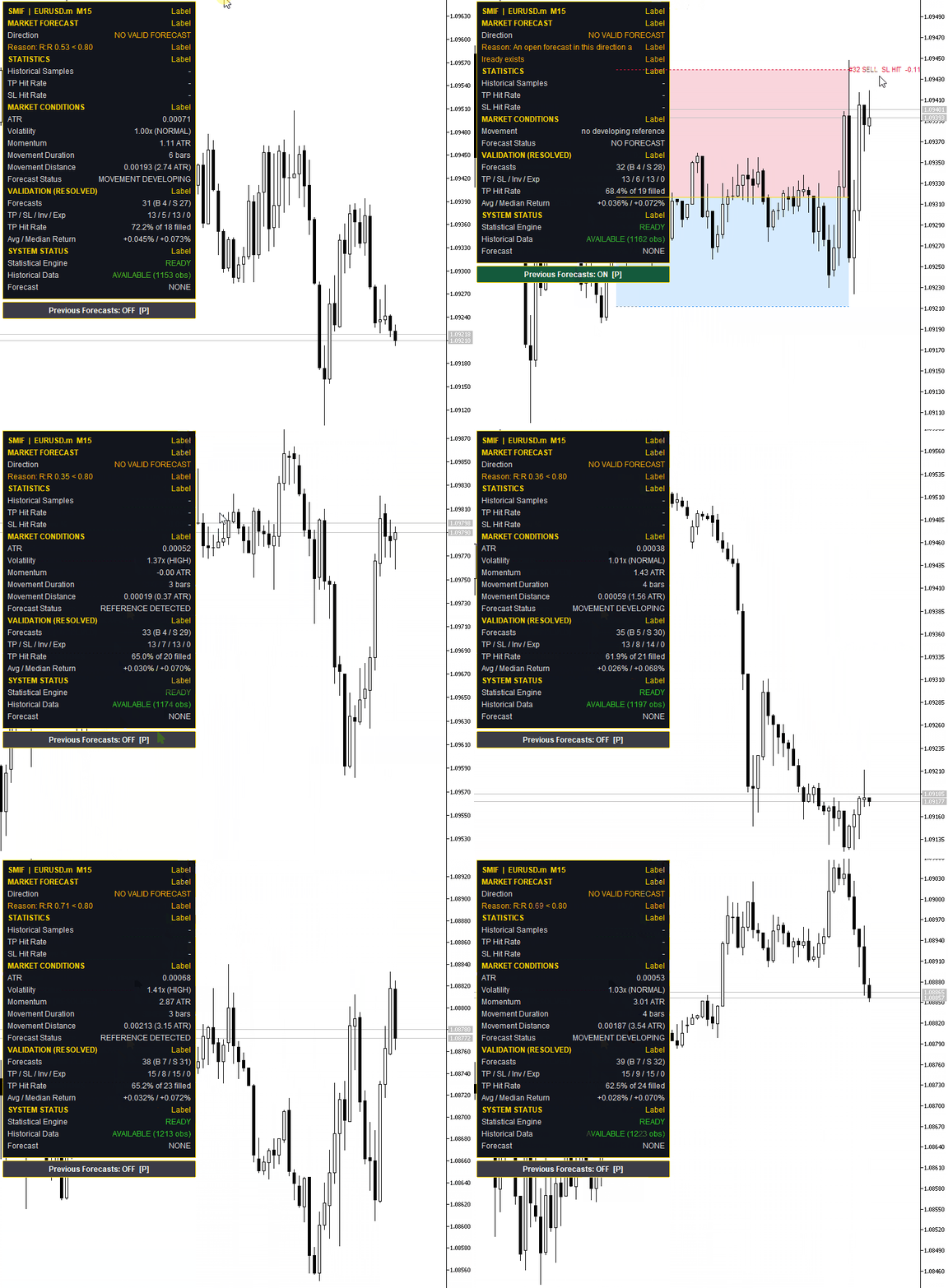
The demonstration below shows the SMIF indicator running on EURUSD, M15, with all the default settings.
Limitations and Proper Use
We need to be clear about what the indicator does not prove. Formal rules make the method repeatable and testable, but repeatable is not the same as profitable. The main limits are listed below, together with what they mean in practice.
- The per-forecast hit rates are in-sample. The levels and the hit rates come from the same neighbors, so they describe how well the levels fit those past cases. The forward validation results, measured on forecasts after their creation, are the better evidence, and even they are measured on one history with one parameter set.
- The rates count filled trades only, and the samples are small. TP and SL rates exclude neighbors that never reached the entry, so the invalidation rate is part of the picture, not a side note. With 20 to 50 filled cases, a rate can move by several points with a single trade, and the confidence interval is wide.
- The replay is an approximation. It works on OHLC bars, resolves bars that touched both levels as a loss, ignores a TP touch on the fill bar, and includes no spread, commission, swap, slippage or gaps. Real execution will be weaker, especially on tight levels.
- The parameters are chosen by hand. ATR thresholds, retracement fractions, percentiles, K and the filter limits are all inputs. This article does not show a walk-forward test, an out-of-sample period or a parameter robustness study, so the results should not be assumed to carry over to other symbols, timeframes or periods.
- The method assumes the past is informative. Similar historical movements are treated as relevant to the current one. ATR normalization makes their scale comparable, but it does not guarantee that the market regime is the same. The observation database also excludes dropped references and movements that never completed, which creates a selection effect.
- In practice, we treat SMIF as a research and decision-support tool, not as a signal service. A sensible workflow is to compare the forward validation results with the in-sample rates, prefer larger samples, subtract the typical spread from the reward-to-risk ratio, and check that the results hold when the main parameters are changed slightly and when the tool is run on a later period it has not seen.
Conclusion
In this article, we built an indicator that treats the turning point of a movement as a statistical question. We defined references, movements and termination with formal, configurable rules. We turned every completed movement into an observation measured in ATR units. We selected the most similar observations for the current movement and read the entry, stop and target from their distributions. We then measured hit rates by replaying the same rules on past bars, one bar at a time, using only bars that were closed at each decision. A state machine followed each forecast until it resolved. Resolved forecasts left the chart automatically, and a single toggle brought them back for review.
The reader leaves with a tool that replaces part of the manual guesswork with measurement. Every level on the chart can be traced back to a distribution, and every hit rate shows the number of cases behind it. The parameters, thresholds and filters are still our choices, and the hit rates are historical frequencies rather than guarantees. When the edge is thin, the filters say so and the dashboard shows NO VALID FORECAST, with the reason. The validation CSV files help us study the method on each symbol, timeframe, session and volatility regime, but a fair judgement still needs out-of-sample testing and realistic trading costs. The same database and replay logic can also serve as the research layer for an Expert Advisor, once the statistics show an edge worth automating.Warning: All rights to these materials are reserved by MetaQuotes Ltd. Copying or reprinting of these materials in whole or in part is prohibited.
This article was written by a user of the site and reflects their personal views. MetaQuotes Ltd is not responsible for the accuracy of the information presented, nor for any consequences resulting from the use of the solutions, strategies or recommendations described.