Hypothesis Testing for Trading Strategies — Proving Whether Your Edge is Real

MetaTrader 5 — Examples | 1 September 2026, 08:39

255

Kayode Michael Oyetunde

Introduction

You have just finished optimizing a strategy in the Strategy Tester. Net profit is positive, the profit factor is comfortably above 1, and the equity curve trends up and to the right. It looks like an edge.

But is it?

A positive backtest is not proof of anything. With enough symbols, timeframes, and parameter combinations, random noise alone will eventually produce a curve that looks exactly like this. The question a serious trader has to answer isn't "did this strategy make money in the past?" — it's "is there statistical evidence that this strategy's returns are different from what pure chance would produce?"

That is a hypothesis testing question, and it has a well-defined, rigorous answer. This article builds that answer from the ground up in pure MQL5 — no external libraries, no Python, no spreadsheets. One thing to flag up front: the toolkit can use two very different data sources. A “significant” result means different things depending on the source. Testing raw price history is not the same claim as testing your strategy's realized trades, even though the same statistical machinery is used. That distinction gets its own section below, and it's worth reading closely before you trust any conclusion the script prints. By the end, you will have a single reusable script, HypothesisTestToolkit.mq5, that:

Pulls returns from either price data or your own deal history
Tests whether the mean return is statistically different from zero (or from a benchmark)
Splits returns into high-volatility and low-volatility regimes and tests whether performance genuinely differs between them
Reports everything — t-statistics, degrees of freedom, p-values, confidence intervals, and plain-language conclusions — straight to the Experts tab

Let's start with why this matters at all.

Why Net Profit, Profit Factor, and Win Rate Aren't Enough

These three numbers dominate most strategy evaluations, and all three share the same flaw: they describe what happened, not how likely it was to happen by chance.

Net profit says nothing about the variance of returns. A strategy that made $10,000 from one lucky trade out of 20 is described identically, by this metric, to one that made $10,000 consistently across 500 trades.
Profit factor (gross profit ÷ gross loss) is sample-size blind. A profit factor of 1.8 computed from 15 trades carries almost no statistical weight; the same 1.8 from 1,500 trades is a very different claim.
Win rate ignores the size of wins versus losses entirely, and again carries no notion of confidence or sample size.

None of these metrics can answer the only question that matters before you risk real capital: if the true underlying edge were exactly zero, how likely is it that random chance alone would produce results this good? That's precisely what a hypothesis test computes.

Parametric vs. Non-Parametric Tests: The Two Tools We Need

There are two broad families of hypothesis tests, and the toolkit implements one test from each family.

Parametric tests (the t-test) assume the underlying data comes from a specific distribution — typically the normal distribution — and compare means. They're powerful (they extract more information from the same data) but sensitive to their assumptions. Trading returns are famously fat-tailed and skewed, so this assumption is often violated to some degree. For large sample sizes, the Central Limit Theorem rescues us somewhat — the sampling distribution of the mean becomes approximately normal even when the underlying returns aren't — which is why t-tests remain useful in practice even on non-normal return series, provided the sample is reasonably large.

Non-parametric tests (the Mann-Whitney U test) make no distributional assumption at all. Instead of comparing means, the Mann-Whitney U test asks whether one sample's values tend to be systematically larger or smaller than another's, based purely on rank ordering. It's less powerful when the normal assumption genuinely holds, but far more robust when it doesn't — which makes it a natural complement to the t-test rather than a replacement for it.

The toolkit runs both, side by side, whenever a two-sample comparison is made. If they agree, you can trust the conclusion with more confidence. If they disagree, that disagreement is itself informative — it usually means outliers or skew are driving the t-test result.

Preparing Clean Return Data

Every test in this toolkit operates on a vector of returns, so getting that vector right is the foundation everything else sits on. The script supports two sources, and it's worth being precise about what each one actually lets you claim, so a significant result isn't mistaken for something it's not:

Directly from market prices, for research purposes — testing whether a market itself has a statistically significant drift, or whether returns genuinely behave differently across volatility regimes, independent of any trading logic.
From a strategy's own deal history, for strategy validation — testing whether the equity-normalized realized profits and losses your strategy actually generated are statistically distinguishable from zero (or from a benchmark).

The two code paths below build the same kind of output — a plain vector of returns — but they are not interchangeable in what they let you conclude.

Important — read this before interpreting any result:

Data source	A "significant" result tells you...
Price data (BuildReturnsFromPrices)	The market itself has a statistically real drift, or its volatility regimes genuinely behave differently — independent of any trading logic.
Deal history (BuildReturnsFromDeals)	Your strategy's realized P&L is statistically distinguishable from zero or from a benchmark.

Every test function downstream (OneSampleTTest, WelchTTest, MannWhitneyU) is completely agnostic to which one produced the vector — the code has no way of knowing or enforcing which claim you're entitled to make. That distinction is entirely on you to keep straight, every single time you read a p-value out of this script.

Log Returns from Price Data

//+---------------------------------------------------------------------+
//|      DATA PREPARATION: build a clean log-return series              |
//| Build log returns from close prices: r_i = ln(close_i / close_{i-1})|
//+---------------------------------------------------------------------+
bool BuildReturnsFromPrices(string sym, ENUM_TIMEFRAMES tf, int bars, vector &returns)
  {
   double close[];
   ArraySetAsSeries(close, false);

   int copied = CopyClose(sym, tf, 0, bars + 1, close);
   if(copied < bars + 1)
     {
      Print("HypothesisTestToolkit: failed to copy price data, copied=", copied,
            " error=", GetLastError());
      return false;
     }

   returns.Resize(bars);
   for(int i = 1; i <= bars; i++)
      returns[i - 1] = MathLog(close[i] / close[i - 1]);

   return true;
  }

We deliberately use logarithmic returns, r_i = ln(close_i / close_{i-1}), rather than simple percentage returns. Log returns are additive across time (the sum of log returns over a period equals the log return of the whole period), which makes them far better behaved for the kind of aggregation and variance calculations hypothesis tests rely on. ArraySetAsSeries(close, false) keeps the array in chronological order (oldest first) so the return calculation walks forward in time correctly.

Per-Trade Returns from Deal History

//+---------------------------------------------------------------------------+
//|Build per-trade percentage returns from closed deals in the account history|
//+---------------------------------------------------------------------------+
bool BuildReturnsFromDeals(datetime from, datetime to, double initBalance, vector &returns)
  {
   if(!HistorySelect(from, to))
     {
      Print("HypothesisTestToolkit: HistorySelect failed, error=", GetLastError());
      return false;
     }

   int total = HistoryDealsTotal();
   double retArr[];
   ArrayResize(retArr, total);
   int count = 0;

   double balance = initBalance;

   for(int i = 0; i < total; i++)
     {
      ulong ticket = HistoryDealGetTicket(i);
      if(ticket == 0)
         continue;

      ENUM_DEAL_ENTRY entry = (ENUM_DEAL_ENTRY)HistoryDealGetInteger(ticket, DEAL_ENTRY);
      if(entry != DEAL_ENTRY_OUT && entry != DEAL_ENTRY_INOUT && entry != DEAL_ENTRY_OUT_BY)
         continue; // only closing deals carry realized P/L

      double profit = HistoryDealGetDouble(ticket, DEAL_PROFIT)
                      + HistoryDealGetDouble(ticket, DEAL_SWAP)
                      + HistoryDealGetDouble(ticket, DEAL_COMMISSION);

      if(balance <= 0.0)
         continue;

      retArr[count++] = profit / balance;
      balance += profit;
     }

   if(count < 2)
     {
      Print("HypothesisTestToolkit: not enough closed deals in the selected history range.");
      return false;
     }

   returns.Resize(count);
   for(int i = 0; i < count; i++)
      returns[i] = retArr[i];

   return true;
  }

Here, each observation is the realized profit of a closing deal (…) normalized by a running notional account balance (seeded by InpInitialBalance). It's worth being precise about what this actually is: it's not a percentage return in the classical sense of price_t / price_{t-1} — it's an equity-normalized realized P&L observation, i.e., realized P&L divided by whatever the running balance happened to be at that point. Because the denominator (balance) changes with every trade, these values are comparable to each other in scale, but they are not price returns. They are closer to “return on running equity” than to “return on a fixed instrument price.”

That framing matters when you interpret Test 1/2 on deal-history data: you're testing whether this equity-normalized P&L stream has a mean distinguishable from zero, not testing a price return per se. This still lets you feed your own live or backtested deal history directly into the same statistical machinery used for price data — just keep the distinction in mind.

The Statistical Math

Before we get to the tests themselves, the script needs a few numerical building blocks that MQL5 doesn't provide natively: the Student's t-distribution and the normal distribution, both needed to turn a test statistic into a p-value.

Log-Gamma and the Incomplete Beta Function

//+------------------------------------------------------------------------+
//|  LOW-LEVEL MATH: log-gamma, incomplete beta, Student-t CDF, erf/normal |
//| Lanczos approximation of the log-gamma function                        |
//+------------------------------------------------------------------------+
double LogGamma(double x)
  {
   static const double g = 7.0;
   static const double coef[9] =
     {
      0.99999999999980993, 676.5203681218851, -1259.1392167224028,
      771.32342877765313, -176.61502916214059, 12.507343278686905,
      -0.13857109526572012, 9.9843695780195716e-6, 1.5056327351493116e-7
     };

   if(x < 0.5)
      return MathLog(M_PI / MathSin(M_PI * x)) - LogGamma(1.0 - x);

   x -= 1.0;
   double a = coef[0];
   double t = x + g + 0.5;
   for(int i = 1; i < 9; i++)
      a += coef[i] / (x + i);

   return 0.5 * MathLog(2.0 * M_PI) + (x + 0.5) * MathLog(t) - t + MathLog(a);
  }

The Student's t cumulative distribution function has a closed form only in terms of the regularized incomplete beta function, I_x(a,b), which in turn is defined using the gamma function. Computing the gamma function directly overflows for even moderate arguments, so we work in log-space using the Lanczos approximation — a standard, numerically stable way to compute ln(Γ(x)) to about 15 significant digits.

//+------------------------------------------------------------------------+
//|Continued fraction used by the regularized incomplete beta function     |
//+------------------------------------------------------------------------+
double BetaCF(double x, double a, double b)
  {
   const int    MAXIT = 200;
   const double EPS   = 3.0e-12;
   const double FPMIN = 1.0e-300;

   double qab = a + b;
   double qap = a + 1.0;
   double qam = a - 1.0;
   double c = 1.0;
   double d = 1.0 - qab * x / qap;
   if(MathAbs(d) < FPMIN)
      d = FPMIN;
   d = 1.0 / d;
   double h = d;

   for(int m = 1; m <= MAXIT; m++)
     {
      int m2 = 2 * m;
      double aa = m * (b - m) * x / ((qam + m2) * (a + m2));
      d = 1.0 + aa * d;
      if(MathAbs(d) < FPMIN)
         d = FPMIN;
      c = 1.0 + aa / c;
      if(MathAbs(c) < FPMIN)
         c = FPMIN;
      d = 1.0 / d;
      h *= d * c;

      aa = -(a + m) * (qab + m) * x / ((a + m2) * (qap + m2));
      d = 1.0 + aa * d;
      if(MathAbs(d) < FPMIN)
         d = FPMIN;
      c = 1.0 + aa / c;
      if(MathAbs(c) < FPMIN)
         c = FPMIN;
      d = 1.0 / d;
      double del = d * c;
      h *= del;

      if(MathAbs(del - 1.0) < EPS)
         break;
     }
   return h;
  }

//+------------------------------------------------------------------------+
//|Regularized incomplete beta function I_x(a,b)                           |
//+------------------------------------------------------------------------+
double IncompleteBeta(double x, double a, double b)
  {
   if(x <= 0.0)
      return 0.0;
   if(x >= 1.0)
      return 1.0;

   double bt = MathExp(LogGamma(a + b) - LogGamma(a) - LogGamma(b) +
                       a * MathLog(x) + b * MathLog(1.0 - x));

   if(x < (a + 1.0) / (a + b + 2.0))
      return bt * BetaCF(x, a, b) / a;
   else
      return 1.0 - bt * BetaCF(1.0 - x, b, a) / b;
  }

BetaCF evaluates a continued fraction that converges quickly on one side of the distribution or the other; IncompleteBeta picks whichever side converges faster and applies the standard symmetry relation if needed. This is the same numerical recipe used inside most statistical software packages under the hood.

From Incomplete Beta to a t-Test p-Value

//+------------------------------------------------------------------------+
//|Student's t cumulative distribution function                            |
//+------------------------------------------------------------------------+
double StudentTCDF(double t, double df)
  {
   double x  = df / (df + t * t);
   double ib = IncompleteBeta(x, df / 2.0, 0.5);
   return (t > 0.0) ? 1.0 - 0.5 * ib : 0.5 * ib;
  }

//+------------------------------------------------------------------------+
//| Two-tailed p-value for a t-statistic                                   |
//+------------------------------------------------------------------------+
double TTestPValueTwoTailed(double t, double df)
  {
   double p = 2.0 * (1.0 - StudentTCDF(MathAbs(t), df));
   if(p < 0.0)
      p = 0.0;
   if(p > 1.0)
      p = 1.0;
   return p;
  }

Once we can evaluate the t-distribution's CDF at any test statistic and degrees of freedom, getting a two-tailed p-value is simple arithmetic: it's twice the probability mass beyond |t| in either tail.

The Normal Distribution (for the Mann-Whitney U Test)

//+------------------------------------------------------------------------+
//| Abramowitz-Stegun approximation of the error function                  |
//+------------------------------------------------------------------------+
double ErfApprox(double x)
  {
   double sign = (x < 0.0) ? -1.0 : 1.0;
   x = MathAbs(x);

   double a1 =  0.254829592, a2 = -0.284496736, a3 = 1.421413741,
          a4 = -1.453152027, a5 =  1.061405429, p  = 0.3275911;

   double t = 1.0 / (1.0 + p * x);
   double y = 1.0 - (((((a5 * t + a4) * t) + a3) * t + a2) * t + a1) * t * MathExp(-x * x);
   return sign * y;
  }

//+------------------------------------------------------------------------+
//|Standard normal cumulative distribution function                        |
//+------------------------------------------------------------------------+
double NormalCDF(double x)
  {
   return 0.5 * (1.0 + ErfApprox(x / MathSqrt(2.0)));
  }

The Mann-Whitney U test's p-value comes from a normal approximation rather than the t-distribution, so we need a standalone normal CDF. ErfApprox is the classic Abramowitz-Stegun polynomial approximation of the error function — accurate to about 7 decimal places, which is more than sufficient here.

Descriptive Statistics and Confidence Intervals

//+------------------------------------------------------------------+
//|      BASIC DESCRIPTIVE STATISTICS & CONFIDENCE INTERVALS         |
//+------------------------------------------------------------------+
double StatMean(const vector &x)
  {
   int n = (int)x.Size();
   if(n == 0)
      return 0.0;
   double s = 0.0;
   for(int i = 0; i < n; i++)
      s += x[i];
   return s / n;
  }

//+------------------------------------------------------------------+
//|Sample variance (Bessel-corrected, n-1 denominator)               |
//+------------------------------------------------------------------+
double StatVariance(const vector &x)
  {
   int n = (int)x.Size();
   if(n < 2)
      return 0.0;
   double m = StatMean(x);
   double s = 0.0;
   for(int i = 0; i < n; i++)
      s += (x[i] - m) * (x[i] - m);
   return s / (n - 1);
  }

//+------------------------------------------------------------------------+
//|Returns the sample standard deviation of x (square root of the variance)|
//+------------------------------------------------------------------------+
double StatStd(const vector &x)
  {
   return MathSqrt(StatVariance(x));
  }

Notice StatVariance divides by n - 1, not n — this is Bessel's correction, which produces an unbiased estimate of the population variance from a sample. Every hypothesis test in the toolkit depends on this being correct, so it's worth implementing explicitly rather than trusting an unknown built-in default.

Every one of these functions takes const vector &x rather than a plain array. This is deliberate: MQL5's vector type carries its own size, supports direct indexing, and — because the parameter is passed by const reference — the function can't accidentally modify the caller's data and doesn't pay the cost of copying it. This pattern (const vector &) is used consistently throughout the toolkit for exactly that reason: statistical functions should be pure, reusable, and cheap to call repeatedly.

Turning Standard Error into a Confidence Interval

//+------------------------------------------------------------------------------------------------+
//|Approximates critical t-value for two-tailed confidence interval using Cornish-Fisher expansion |
//+------------------------------------------------------------------------------------------------+
double CriticalValueT(double alpha, double df)
  {
   double z = 1.95996; // Default ~95% CI (alpha = 0.05)
   if(MathAbs(alpha - 0.01) < 0.005)
      z = 2.57583; // 99% CI
   if(MathAbs(alpha - 0.10) < 0.005)
      z = 1.64485; // 90% CI

   return z + (z * z * z + z) / (4.0 * df);
  }

//+-----------------------------------------------------------------------+
//|Computes lower and upper confidence interval bounds for the mean return|
//+-----------------------------------------------------------------------+
void MeanConfidenceInterval(const vector &x, double alpha, double &lowerBound, double &upperBound)
  {
   int n = (int)x.Size();
   if(n < 2)
     {
      lowerBound = 0.0;
      upperBound = 0.0;
      return;
     }

   double mean = StatMean(x);
   double se   = StatStd(x) / MathSqrt((double)n);
   double tCrit = CriticalValueT(alpha, n - 1);

   lowerBound = mean - tCrit * se;
   upperBound = mean + tCrit * se;
  }

A p-value tells you whether an effect is statistically distinguishable from zero, but it doesn't tell you how big the effect plausibly is. A confidence interval does. MeanConfidenceInterval computes the standard error of the mean (std / sqrt(n)) and multiplies it by a critical value to build an interval that — under repeated sampling — would contain the true mean return (1 - alpha) × 100% of the time.

CriticalValueT deserves an honest caveat: rather than inverting the full incomplete beta function a second time (expensive and unnecessary for this purpose), it starts from the standard normal critical value for the requested alpha and applies a first-order correction, z + (z³ + z)/(4·df), which pulls the normal critical value out toward the fatter tails of the t-distribution for small samples. This converges toward the exact t critical value as df grows, and is reasonably close for moderate-to-large sample sizes — good enough to give a sense of the range for a report-level confidence interval. It is, however, only an approximation, and it's less reliable the smaller your sample gets. For formal small-sample inference (n well under 30), or anywhere the exact width of the interval matters, treat the bound this produces as indicative rather than precise, and consider computing an exact t-quantile separately if the decision depends on it.

How to read this in practice: if your 95% confidence interval for mean return is approximately [0.00012, 0.00089], you can say "we're roughly 95% confident the true mean return is positive and somewhere near this range" — which, even as an approximation, is a far more honest and useful statement than a single backtested average.

Splitting Returns into Volatility Regimes

A strategy that performs beautifully in calm markets and falls apart in turbulent ones doesn't have one edge — it has a conditional edge, and you need to know that before you trade it live through a regime change. The toolkit detects regimes automatically using rolling volatility.

//+---------------------------------------------------------------------+
//|      REGIME SPLITTING (rolling volatility, high vs low)             |
//| Rolling standard deviation over a fixed window; vol[i] covers       |
//| returns[i .. i+window-1], so vol[i] "belongs" to returns[i+window-1]|
//+---------------------------------------------------------------------+
void RollingVolatility(const vector &returns, int window, vector &vol)
  {
   int n = (int)returns.Size();
   int m = n - window + 1;
   if(m < 1)
     {
      vol.Resize(0);
      return;
     }

   vol.Resize(m);
   vector w;
   w.Resize(window);

   for(int i = 0; i < m; i++)
     {
      for(int k = 0; k < window; k++)
         w[k] = returns[i + k];
      vol[i] = StatStd(w);
     }
  }

For every position in the return series, we slide a window of InpVolWindow bars and compute the standard deviation inside it. The result, vol[i], is anchored to returns[i + window - 1] — i.e., it describes the volatility up to and including that return, not a look-ahead average.

//+---------------------------------------------------------------------+
//| Splits returns into a High-volatility and a Low-volatility regime   |
//| using a percentile threshold on rolling volatility                  |
//+---------------------------------------------------------------------+
void SplitByRegime(const vector &returns, int window, double percentile,
                   vector &highRegime, vector &lowRegime)
  {
   vector vol;
   RollingVolatility(returns, window, vol);

   int m = (int)vol.Size();
   if(m < 2)
     {
      highRegime.Resize(0);
      lowRegime.Resize(0);
      return;
     }

   double threshold = Percentile(vol, percentile);

   double highArr[], lowArr[];
   ArrayResize(highArr, m);
   ArrayResize(lowArr, m);
   int hCount = 0, lCount = 0;

   for(int i = 0; i < m; i++)
     {
      int idx = i + window - 1;
      double r = returns[idx];
      if(vol[i] >= threshold)
         highArr[hCount++] = r;
      else
         lowArr[lCount++]  = r;
     }

   highRegime.Resize(hCount);
   for(int i = 0; i < hCount; i++)
      highRegime[i] = highArr[i];

   lowRegime.Resize(lCount);
   for(int i = 0; i < lCount; i++)
      lowRegime[i] = lowArr[i];
  }

Percentile (using ArraySort and linear interpolation between ranks) finds the volatility threshold that splits the sample at InpVolPercentile — 50 by default, i.e., a straight median split into "High-vol" and "Low-vol" halves. Every return is then bucketed into one regime or the other, producing exactly the two vectors we need for a two-sample comparison.

The Hypothesis Tests

This is the core of the toolkit — three tests, each answering a different question.

Tests 1 & 2: One-Sample t-Test

Before looking at what this test reports, a quick reminder: if the vector you fed it came from price data, a rejection of H₀ here is a statement about the market's drift, not about any strategy; if it came from deal history, it's a statement about your strategy's edge. The math below doesn't distinguish the two — you have to.

One more matters before interpreting any t-statistic: observations should be independent. In financial return series this is often violated because of serial correlation, volatility clustering, and winning or losing streaks. When dependence is present, the reported p-values tend to be overly optimistic. A fuller discussion appears later under 'Two Assumptions Worth Knowing Before You Trust a p-Value,' but keep this limitation in mind before interpreting any significance result.

//+------------------------------------------------------------------+
//|                        HYPOTHESIS TESTS                          |
//|          One-sample t-test: H0: mean(x) = mu0                    |
//+------------------------------------------------------------------+
void OneSampleTTest(const vector &x, double mu0, double &tStat, double &df, double &pValue)
  {
   int n = (int)x.Size();
   double mean = StatMean(x);
   double sd   = StatStd(x);
   double se   = sd / MathSqrt((double)n);

   tStat = (se > 0.0) ? (mean - mu0) / se : 0.0;
   df    = n - 1;
   pValue = TTestPValueTwoTailed(tStat, df);
  }

This is the workhorse of the whole toolkit. It tests the null hypothesis H₀: the true mean return equals mu0. The script calls it twice:

Test 1 — mu0 = 0. This is the fundamental "is there an edge at all?" test. A small p-value here (below your chosen InpSignificanceLevel) is evidence the observed mean return is unlikely to have arisen from a strategy with zero true edge.
Test 2 — mu0 = InpBenchmarkReturn. The same math, but against any benchmark you supply (buy-and-hold return, a competing strategy's mean return, a required hurdle rate, etc.), letting you test outperformance rather than mere profitability.

The t-statistic itself is just "how many standard errors is the sample mean away from the hypothesized value" — the more standard errors, the less plausible it is that the true mean is actually mu0.

Test 3: Welch's Two-Sample t-Test

//+---------------------------------------------------------------------+
//| Welch's two-sample t-test (unequal variances): H0: mean(a) = mean(b)|
//+---------------------------------------------------------------------+
void WelchTTest(const vector &a, const vector &b, double &tStat, double &df, double &pValue)
  {
   int n1 = (int)a.Size();
   int n2 = (int)b.Size();

   double m1 = StatMean(a), m2 = StatMean(b);
   double v1 = StatVariance(a), v2 = StatVariance(b);

   double se = MathSqrt(v1 / n1 + v2 / n2);
   tStat = (se > 0.0) ? (m1 - m2) / se : 0.0;

   double num = MathPow(v1 / n1 + v2 / n2, 2);
   double den = MathPow(v1 / n1, 2) / (n1 - 1) + MathPow(v2 / n2, 2) / (n2 - 1);
   df = (den > 0.0) ? num / den : (n1 + n2 - 2);

   pValue = TTestPValueTwoTailed(tStat, df);
  }

Applied to the high-volatility and low-volatility regime vectors, this tests H₀: mean(high-vol) = mean(low-vol). We deliberately use Welch's version of the two-sample t-test rather than the classic Student's version, because Welch's test does not assume the two groups have equal variance — and volatility regimes almost by definition have unequal variance. Welch's correction shows up in the df calculation: instead of a fixed n1 + n2 - 2, degrees of freedom are computed from the Satterthwaite approximation, which shrinks toward the smaller effective sample size when variances differ substantially.

Test 4: Mann-Whitney U Test

//+---------------------------------------------------------------------+
//| Mann-Whitney U test with tie correction and normal approximation    |
//|H0: the two samples come from the same distribution                  |
//+---------------------------------------------------------------------+
void MannWhitneyU(const vector &a, const vector &b, double &uStat, double &zStat, double &pValue)
  {
   const double TIE_EPS = 1.0e-9; // tolerance for treating two returns as tied

   int n1 = (int)a.Size();
   int n2 = (int)b.Size();
   int n  = n1 + n2;

   double values[];
   int    groups[];
   ArrayResize(values, n);
   ArrayResize(groups, n);

   for(int i = 0; i < n1; i++)
     {
      values[i]      = a[i];
      groups[i]      = 1;
     }
   for(int i = 0; i < n2; i++)
     {
      values[n1 + i] = b[i];
      groups[n1 + i] = 2;
     }

//--- index sort (insertion sort; fine for typical sample sizes)
   int order[];
   ArrayResize(order, n);
   for(int i = 0; i < n; i++)
      order[i] = i;

   for(int i = 1; i < n; i++)
     {
      int key = order[i];
      double keyVal = values[key];
      int j = i - 1;
      while(j >= 0 && values[order[j]] > keyVal)
        {
         order[j + 1] = order[j];
         j--;
        }
      order[j + 1] = key;
     }

//--- assign ranks, averaging ties, and accumulate the tie-correction sum
   double ranks[];
   ArrayResize(ranks, n);
   double sumT = 0.0;

   int i = 0;
   while(i < n)
     {
      int j = i;
      while(j + 1 < n && MathAbs(values[order[j + 1]] - values[order[i]]) <= TIE_EPS)
         j++;

      double avgRank = (i + 1 + j + 1) / 2.0; // 1-based ranks
      int tieCount = j - i + 1;
      for(int k = i; k <= j; k++)
         ranks[order[k]] = avgRank;

      if(tieCount > 1)
         sumT += MathPow((double)tieCount, 3) - tieCount;
      i = j + 1;
     }

   double R1 = 0.0;
   for(int k = 0; k < n; k++)
      if(groups[k] == 1)
         R1 += ranks[k];

   double U1 = R1 - n1 * (n1 + 1) / 2.0;
   double U2 = (double)n1 * n2 - U1;
   uStat = MathMin(U1, U2);

   double muU = n1 * n2 / 2.0;
   double sigmaU2 = ((double)n1 * n2 / 12.0) * ((n + 1) - sumT / ((double)n * (n - 1)));
   double sigmaU  = MathSqrt(MathMax(sigmaU2, 0.0));

   double diff = U1 - muU;
   double cc = (diff > 0.0) ? -0.5 : (diff < 0.0 ? 0.5 : 0.0); // continuity correction

   zStat = (sigmaU > 0.0) ? (diff + cc) / sigmaU : 0.0;

   pValue = 2.0 * (1.0 - NormalCDF(MathAbs(zStat)));
   if(pValue < 0.0)
      pValue = 0.0;
   if(pValue > 1.0)
      pValue = 1.0;
  }

This is the non-parametric complement to Test 3, testing H₀: the high-vol and low-vol returns are drawn from the same distribution — equivalently, that a randomly chosen value from one regime is equally likely to be larger or smaller than a randomly chosen value from the other — without assuming normality. Walking through the mechanics:

Combine and rank. Both regime vectors are merged into one array, sorted, and every value is assigned a rank from 1 to n1 + n2. Tied values receive the average of the ranks they span — this is the standard, statistically correct way to handle ties rather than arbitrarily breaking them.
Sum ranks per group. R1, the sum of ranks belonging to the first group, is converted into U1 = R1 - n1(n1+1)/2, which counts (in effect) how many times a value from group 1 beat a value from group 2 across all pairwise comparisons. U2 is the complementary count, and U = min(U1, U2).
Tie correction. Because tied ranks reduce the variance of U under the null hypothesis, the toolkit explicitly accumulates Σ(t³ - t) across every group of tied values and folds it into the variance formula:

double sigmaU2 = ((double)n1 * n2 / 12.0) * ((n + 1) - sumT / ((double)n * (n - 1)));

Skipping this correction — which many simplified implementations do — silently overstates significance whenever the return series has repeated values (common with rounded price data or identical-lot-size trade outcomes).

Normal approximation with continuity correction. For reasonably sized samples, U is approximately normal, so a z-score (with a ±0.5 continuity correction, since U is technically discrete) is converted straight into a two-tailed p-value via NormalCDF.

Why run both Test 3 and Test 4?

If the t-test and the Mann-Whitney U test agree, you have two independent lines of evidence pointing the same way. If they disagree — say, the t-test is significant but Mann-Whitney isn't — it's a strong signal that a handful of outlier trades or bars are driving the mean-based result, rather than a broad, rank-consistent tendency for one regime's returns to run higher or lower than the other's. It's worth being precise about what Mann-Whitney actually tests here: it doesn't test medians directly, and it doesn't claim the 'typical' return differs in some intuitive sense — it tests whether values from one regime are stochastically larger or smaller than values from the other, based purely on rank ordering. A disagreement between the two tests tells you the mean-based conclusion is fragile and likely outlier-driven, not that you've proven "nothing is different" — that's exactly the kind of nuance you want in hand before sizing a position around a "regime edge."

Two Assumptions Worth Knowing Before You Trust a p-Value

Every test above is mathematically correct, but correctness of the math doesn't excuse you from understanding what the tests assume. Two limitations are important enough to call out explicitly.

Multiple testing inflates your false-positive rate. The script runs four hypothesis tests on the same underlying data. Each one is calibrated so that, on its own, a true null hypothesis is falsely rejected only α of the time — 5% at the default setting. But run four such tests, and the probability that at least one comes back "significant" purely by chance is roughly 1 - (1 - α)⁴ ≈ 18.6% at α = 0.05 — well above the 5% a single test promises. If you want to guard against this, the simplest fix is a Bonferroni correction: divide your significance level by the number of tests before comparing p-values against it (α/4 ≈ 0.0125 here, instead of 0.05). The toolkit deliberately doesn't apply this automatically — which test results you consider jointly is a judgment call that depends on what you're asking — but treat a single "significant" result out of four as noticeably weaker evidence than the raw p-value alone suggests.

Both tests assume independent observations. In trading, this assumption is violated far more often than most people expect. The t-test and the Mann-Whitney U test are both built on the premise that each return in the sample is drawn independently of the others. Trading returns routinely fail this: a trend-following system that rides one move across many consecutive bars, a strategy with winning or losing streaks, or even ordinary price data with volatility clustering all produce serially correlated returns, where this observation's outcome is not independent of the last one's.

This isn't a minor caveat — it's close to the default state of most retail and even institutional return series, and autocorrelation of this kind systematically inflates t-statistics and understates true p-values, making a strategy (or a market) look far more statistically significant than the data actually supports. If your returns show any persistence — win/loss streaks, trending behavior, volatility clustering — treat every p-value in this report as optimistic, and corroborate it with out-of-sample testing rather than acting on a single significant in-sample result. When in doubt, assume dependence is present until you've specifically checked for it.

Reporting: Vectors, a Matrix, and a Plain-Language Verdict

//+------------------------------------------------------------------------------------+
//|    MATRIX-BASED SUMMARY (demonstrates the matrix type)                             |
//| Builds a 2x4 matrix: rows = [High regime, Low regime], cols = [mean, std, min, max]|
//+------------------------------------------------------------------------------------+
matrix BuildSummaryMatrix(const vector &high, const vector &low)
  {
   matrix m(2, 4);

   m[0][0] = StatMean(high);
   m[0][1] = StatStd(high);
   m[0][2] = high.Min();
   m[0][3] = high.Max();
   m[1][0] = StatMean(low);
   m[1][1] = StatStd(low);
   m[1][2] = low.Min();
   m[1][3] = low.Max();

   return m;
  }

Alongside vector, MQL5's matrix type is a natural fit for tabular summary statistics. Here, a 2×4 matrix packs mean, standard deviation, minimum, and maximum for both regimes into one structure — rows for groups, columns for statistics — which is both efficient (single allocation, contiguous memory) and readable at the call site (summary[0][1] is unambiguously "high-vol regime, standard deviation").

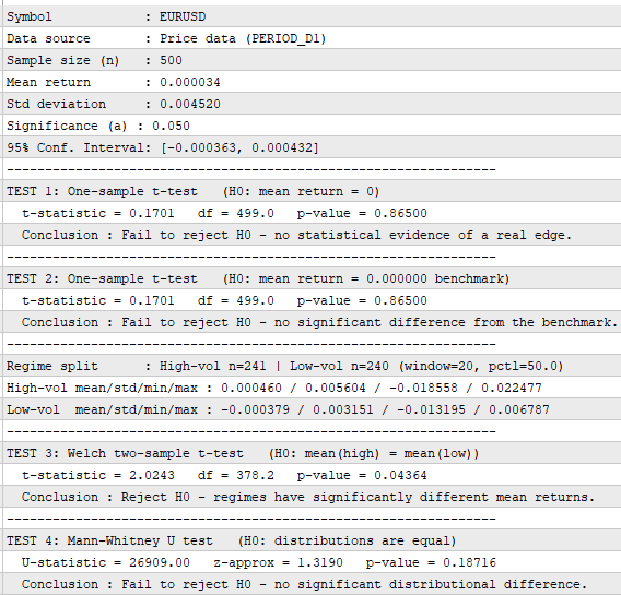
Everything converges in PrintReport, which pulls together the descriptive statistics, the confidence interval, and the outcome of all four tests into a single formatted block written to the Experts tab — including an explicit Reject H₀ / Fail to reject H₀ conclusion for every test, so you don't have to mentally compare a p-value against alpha yourself every time you run it.

Print("  Conclusion : ", (p1 < alpha
      ? "Reject H0 - mean return is statistically different from zero."
      : "Fail to reject H0 - no statistical evidence of a real edge."));

A word on interpretation: "fail to reject H₀" is not the same as "the strategy has no edge" — it means the data collected so far isn't enough to distinguish the strategy's performance from pure chance at your chosen confidence level. That could mean there's genuinely no edge, or it could mean your sample is too small to detect a real but modest one. More data (a longer backtest, a longer live track record) is the only way to resolve that ambiguity, which is itself a useful, honest conclusion for a trader to sit with before committing capital.

Putting It Together: OnStart()

//+------------------------------------------------------------------+
//|                      SCRIPT ENTRY POINT                          |
//+------------------------------------------------------------------+
void OnStart()
  {
   string sym = (InpSymbol == "") ? _Symbol : InpSymbol;

   vector returns;
   bool ok = false;

   if(InpUseDealHistory)
     {
      datetime to   = (InpHistoryTo == 0) ? TimeCurrent() : InpHistoryTo;
      datetime from = (InpHistoryFrom == 0) ? (to - 30 * 24 * 60 * 60) : InpHistoryFrom;
      ok = BuildReturnsFromDeals(from, to, InpInitialBalance, returns);
     }
   else
     {
      ok = BuildReturnsFromPrices(sym, InpTimeframe, InpBars, returns);
     }

   if(!ok || (int)returns.Size() < 10)
     {
      Print("HypothesisTestToolkit: insufficient data to run tests. Aborting.");
      return;
     }

   int n = (int)returns.Size();

//--- Test 1: returns vs zero
   double t1, df1, p1;
   OneSampleTTest(returns, 0.0, t1, df1, p1);

//--- Test 2: returns vs a user-defined benchmark mean
   double t2, df2, p2;
   OneSampleTTest(returns, InpBenchmarkReturn, t2, df2, p2);

//--- Regime split by rolling volatility
   vector highRegime, lowRegime;
   SplitByRegime(returns, InpVolWindow, InpVolPercentile, highRegime, lowRegime);
   bool haveRegimes = ((int)highRegime.Size() >= 5 && (int)lowRegime.Size() >= 5);

   double t3 = 0.0, df3 = 0.0, p3 = 1.0;
   double u4 = 0.0, z4 = 0.0, p4 = 1.0;

   if(haveRegimes)
     {
      WelchTTest(highRegime, lowRegime, t3, df3, p3);
      MannWhitneyU(highRegime, lowRegime, u4, z4, p4);
     }

   PrintReport(sym, n, returns,
               t1, df1, p1, t2, df2, p2,
               highRegime, lowRegime, haveRegimes,
               t3, df3, p3, u4, z4, p4);
  }
//+------------------------------------------------------------------+

OnStart is deliberately thin — it's an orchestration layer, not where any statistics happen. It picks a data source, builds the return vector, guards against too-small samples (fewer than 10 returns isn't enough to say anything meaningful), runs all four tests, and hands everything to PrintReport. Every function it calls takes and returns simple, self-contained vector / matrix arguments, which is exactly what makes this toolkit reusable — you can lift OneSampleTTest, WelchTTest, or MannWhitneyU straight into an Expert Advisor or another script without touching a single line of their implementation.

Running the Toolkit

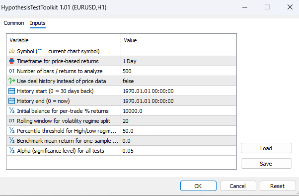
Attach HypothesisTestToolkit.mq5 to any chart as a script. The input dialog lets you configure:

Data source — live price bars (InpTimeframe, InpBars) or your own deal history (InpUseDealHistory, InpHistoryFrom/To, InpInitialBalance)
Regime detection — InpVolWindow (how many bars define "recent volatility") and InpVolPercentile (where to draw the High/Low split — 50 for a median split, higher to isolate only the most extreme volatility spikes)
Statistical rigor — InpSignificanceLevel, the alpha threshold every conclusion is measured against (0.05 is conventional; use 0.01 if you want a stricter bar before trusting a result)

The script's input dialog

Once run, the Experts tab prints the full report — sample size, mean, standard deviation, confidence interval, and all four tests with their conclusions.

Script Expert Tab

To see the regime split visually before trusting the numbers, it helps to look at the price series with the high- and low-volatility windows shaded.

Conclusion

Net profit and profit factor tell you what a strategy did. Hypothesis tests tell you how much you should believe it. This toolkit gives you both halves of that picture: a parametric t-test for when you can trust the normal approximation, a non-parametric Mann-Whitney U test for when you can't, and a regime-splitting framework that stops you from trusting an "edge" that's really just one lucky volatility environment.

None of this replaces good trading judgment — a statistically significant edge with two years of daily data can still evaporate in live trading, and a "fail to reject" result on a short backtest doesn't necessarily mean the strategy is worthless. What it does is remove the guesswork from the first question you should always ask about a backtest: is there any real evidence here at all, or am I just looking at noise that happened to go up?

From here, the same const vector & functions built in this article — OneSampleTTest, WelchTTest, MannWhitneyU, MeanConfidenceInterval — are ready to drop directly into an Expert Advisor for live, rolling statistical monitoring of a strategy's edge, or into a batch script that walks an entire symbol list and evaluates strategies using statistical significance together with traditional performance metrics, rather than profit alone. Whichever way you use them, keep track of which mode produced your numbers — a market-level finding from price data and a strategy-level finding from your deal history are two different claims, and confusing one for the other is the easiest way to misread this entire report.

Attached files |

Download ZIP

HypothesisTestToolkit.mq5 (24.96 KB)

Warning: All rights to these materials are reserved by MetaQuotes Ltd. Copying or reprinting of these materials in whole or in part is prohibited.

This article was written by a user of the site and reflects their personal views. MetaQuotes Ltd is not responsible for the accuracy of the information presented, nor for any consequences resulting from the use of the solutions, strategies or recommendations described.