Neural Networks in Trading: Robust Trading Signals in Any Market Regime (Conclusion)

MetaTrader 5 — Trading systems | 6 October 2026, 11:16

133

Dmitriy Gizlyk

Introduction

Financial markets are governed by the laws of change. Today they may show steady growth, but tomorrow they may react violently to even the slightest external stimulus. New instruments, regulatory initiatives, macroeconomic shocks, and even social sentiment — all of these change the market landscape just as dramatically as the construction of a new highway reshapes traffic flows in a city. That is precisely why classical forecasting algorithms often lose their effectiveness as soon as they encounter new conditions not present in the training set.

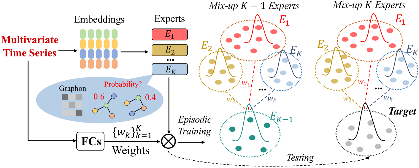
The ST-Expert framework was proposed as one possible solution to this problem. Its central idea is simple and, at the same time, profound. Instead of relying on a single, one-size-fits-all strategy, it forms an ensemble of experts, each specializing in its own segment of market dynamics. This approach can be compared to managing an investment portfolio. An experienced manager does not have a single strategy that works in every situation, but rather a whole set of tools. Some perform better during periods of a steady trend, others generate profits in highly volatile conditions, and still others help preserve capital during a prolonged sideways market. Much like such a portfolio, ST-Expert allocates attention among its experts and forms a balanced solution for new market conditions.

The main advantage of this approach is its robustness. Unlike models that encode rigid relationships between assets and become ineffective when those relationships change, ST-Expert is able to adapt. Its architecture is built around a layer of expert graphons that act as generators of connections between assets. Each graphon forms its own representation of how markets or individual instruments might interact, and the mixing module dynamically selects a combination of experts based on the current situation.

Architecturally, the framework is based on the principle of a mixture of experts (Mixture of Experts). It is based not on a single super-expert, but on an entire ensemble of models trained on various time intervals and scenarios. Episodic training, in which the model is deliberately subjected to a variety of stress tests, becomes a crucial part of the process. The data are divided into different market regimes, such as trend, correction, or flat phases. Then a task is formulated in which each expert is trained under specific conditions. At the same time, the mixing module learns to combine experts to achieve maximum efficiency. This is similar to training a trader on historical data. The trader learns to make decisions in conditions of incomplete information and unpredictable changes. And that is exactly what makes the trader experienced.

From a technical standpoint, the ST-Expert architecture is a multi-layered structure. Raw time series are first converted into embeddings, and are then fed into expert blocks, each of which constructs its own representation of hidden relationships. Next, the mixing module comes into play and determines the weight of each expert for the given market state. The result is a dynamic forecasting system that, rather than searching for a universal formula, balances between different strategies. Like a portfolio manager who, every morning, selects the instruments that are relevant specifically for that day.

This approach combines three key qualities. First, it is flexibility. An expert layer can be integrated into virtually any modern architecture without disrupting the underlying structure. Second, there is robustness. Unlike traditional models, which tend to get stuck on a single pattern, ST-Expert maintains its accuracy even when the market backdrop changes. And finally, there is efficiency. This expansion of capabilities is achieved without an excessive increase in the number of parameters. This makes the framework practical for real-world financial systems, where accuracy and speed are critical.

What makes ST-Expert especially distinctive is its cost-efficiency of implementation. Robustness is usually achieved at the cost of increased computational complexity. More parameters, more data, more time. Here, by contrast, gains are achieved without a drastic increase in costs. In terms of financial markets, this can be compared to an investment strategy that delivers high returns with moderate risk and minimal costs.

The author’s visualization of the ST-Expert framework is shown below.

Author’s visualization of the ST-Expert framework

In our previous work, we have already come a long way — from the theoretical foundations to the practical implementation of the ST-Expert framework. And before we move forward, it is worth taking a moment to look back and systematize what we have covered, so we can better appreciate the scale of the work done and see what opportunities lie ahead.

Right at the beginning, we examined the principle of the mixture of experts in detail. This approach is similar to a trader's diversified portfolio. Each expert is responsible for its own niche, processes specific patterns, and does so without interfering with the others.

Next, we moved from abstract architectural ideas to concrete algorithmic solutions. In practice, this took the form of implementing a set of expert graphons, each of which develops its own understanding of the structure and relationships within the data. Special attention was paid to the mixing module — the core of the entire system. It is this module that provides the key advantage of ST-Expert: the ability to dynamically select experts best suited to a specific market situation. It is like an experienced portfolio manager who can switch from one strategy to another at any time while maintaining a balance between risk and return.

Implementation has shown that the framework does not merely analyze historical data — it can adapt to the transformation of that data. This is especially important for financial markets, where changes occur rapidly and outdated strategies can prove costly. The system's effective adaptability makes it possible to forecast market movements with high accuracy, minimize losses, and capitalize on new opportunities.

The path we have taken has laid the foundation for further work.

Global-Local Attention

In the previous article, we discussed in detail and justified the decisions regarding the implementation of the ST-Expert framework's approaches into the Extralonger architecture. The main goal was to integrate graphons into the Transformer architecture to enhance the model's ability to analyze complex relationships in financial markets. In practice, we implemented full and sparse attention objects, which allowed us to work flexibly with information at different levels of the data hierarchy.

Extralonger places special emphasis on the global-local attention object. It enables two modules to operate in parallel — a global module capable of identifying large-scale patterns, and a local module that focuses on details and anomalies. This approach makes it possible to simultaneously track general market trends and pick up on small signals that can be critical for short-term trading.

To facilitate the integration of this concept into the familiar linear model architecture, we are developing a new global-local attention module based on graphons. This module organizes the operation of global and local attention objects in parallel information streams, followed by adaptive mixing of the results, thereby providing a more accurate and flexible representation of information.

The CNeuronGlobLocGraphAtt class can be thought of as an experienced trader who simultaneously tracks long-term trends and picks up on short-term signals. It is built on the basis of multi-head pooling, inheriting the capabilities of the CNeuronMHAttentionPooling object, which provides a solid foundation for flexible data processing.

class CNeuronGlobLocGraphAtt  :  public CNeuronMHAttentionPooling
  {
protected:
   CNeuronGraphAttention         cGlobal;
   CNeuronSparseGraphAttention   cLocal;
   CNeuronBaseOCL                cConcat;
   //---
   virtual bool      feedForward(CNeuronBaseOCL *NeuronOCL) override;
   virtual bool      updateInputWeights(CNeuronBaseOCL *NeuronOCL) override;
   virtual bool      calcInputGradients(CNeuronBaseOCL *NeuronOCL) override;

public:
                     CNeuronGlobLocGraphAtt(void) {};
                    ~CNeuronGlobLocGraphAtt(void) {};
   virtual bool      Init(uint numOutputs, uint myIndex, COpenCLMy *open_cl,
                          uint units, uint window, uint experts, float dropout,
                          uint emb_dimension, uint sparse_dimension,
                          ENUM_OPTIMIZATION optimization_type, uint batch);
   //---
   virtual int       Type(void) override const   {  return defNeuronGlobLocGraphAtt;   }
   //--- methods for working with files
   virtual bool      Save(int const file_handle) override;
   virtual bool      Load(int const file_handle) override;
   //---
   virtual bool      WeightsUpdate(CNeuronBaseOCL *source, float tau) override;
   virtual void      SetOpenCL(COpenCLMy *obj) override;
   virtual void      SetActivationFunction(ENUM_ACTIVATION value) override { };
   virtual void      TrainMode(bool flag) override;
  };

There are two key components within the class: cGlobal and cLocal. The first, like a senior analyst who sees the market as a whole, reviews the entire data sequence, identifies general patterns and long-term trends, and helps build strategic forecasts. The second acts like a quick tactician, focusing on immediate events and anomalies that can instantly affect the trader's position.

All internal module components are declared as direct class members, which allows us to leave the class's constructor and destructor empty. Initialization takes place in the Init method. This approach is reminiscent of an experienced trader who enters the market with a ready-made team of analysts. Every specialist knows their role. And the manager's job is to assign them the right roles and organize their collaboration.

bool CNeuronGlobLocGraphAtt::Init(uint numOutputs, uint myIndex, COpenCLMy *open_cl,
                                  uint units, uint window, uint experts, float dropout,
                                  uint emb_dimension, uint sparse_dimension,
                                  ENUM_OPTIMIZATION optimization_type, uint batch)
  {
   if(!CNeuronMHAttentionPooling::Init(numOutputs, myIndex, open_cl, window, units,
                                       2, optimization_type, batch))
      return false;

The Init method is responsible for configuring the architecture of our global-local attention module. First, the initialization method of the parent class CNeuronMHAttentionPooling is called. If errors occur at this stage, the process stops. It's like checking an asset's fundamentals before opening a position — without a solid foundation, there's no point in proceeding.

After the base initialization completes successfully, initialization of the internal objects begins. First, cGlobal is configured, which is responsible for global attention. It processes the entire data sequence and builds a strategic picture of the market, identifying long-term trends and patterns. If this component fails to initialize, the module simply cannot continue to function, which underscores the critical importance of global analysis.

   int index = 0;
   if(!cGlobal.Init(0, index, OpenCL, iUnits, iWindow, emb_dimension, experts, dropout,
                    optimization, iBatch))
      return false;

Next, cLocal, a local attention object, is created. It focuses on recent events and sparse patterns, allowing the model to detect important signals and anomalies that might be overlooked by global analysis. Initialization of cLocal is also checked for correctness — if an error occurs, the module does not start, so as not to expose the system to incorrect decisions. Like a trader who won't open a position without reliable data.

   index++;
   if(!cLocal.Init(0, index, OpenCL, iUnits, iWindow, experts, dropout, emb_dimension,
                   sparse_dimension, optimization, iBatch))
      return false;

Finally, the results of global and local attention are combined in cConcat. It is simply a storage object for the concatenated tensor of results from two views of the market. We plan to perform the actual mixing into the final value using the parent class.

   index++;
   if(!cConcat.Init(0, index, OpenCL, 2 * iWindow * iUnits, optimization, iBatch))
      return false;
   cConcat.SetActivationFunction(None);
//---
   return true;
  }

If all steps are completed successfully, the Init method returns true, indicating that the module is ready for operation. Otherwise, initialization is terminated, which ensures the stability and reliability of the model's operation.

The result is a complete architecture in which global and local attention operate in parallel streams, and adaptive mixing ensures accurate and flexible interpretation of market data. The module becomes a dynamic tool capable of both seeing the strategic picture and responding to short-term changes — just like an experienced trader with a finger on the pulse of the market.

After the object has been successfully initialized, the next step is to set up the forward pass of data through the module, which is implemented in the feedForward method. This stage can be thought of as a trader working in real time. Market signals come in continuously, and the system must process them instantly, combining strategic vision with a response to short-term fluctuations.

bool CNeuronGlobLocGraphAtt::feedForward(CNeuronBaseOCL *NeuronOCL)
  {
   if(!cGlobal.FeedForward(NeuronOCL))
      return false;

First, the data passes through the global attention object cGlobal, which provides an overall view of the market and identifies long-term trends and structural patterns. If errors occur at this stage, the forward pass is interrupted, since without the global context, further analysis becomes meaningless — much like a portfolio strategy without an understanding of macroeconomic conditions.

The information is then sent to the local attention object cLocal, which identifies key details, subtle signals, and local anomalies. This component operates in parallel with the global component, focusing on the events that may have an immediate impact on the model's position.

   if(!cLocal.FeedForward(NeuronOCL))
      return false;

After processing by each module, their outputs are concatenated for each individual sequence element.

   if(!Concat(cGlobal.getOutput(), cLocal.getOutput(), cConcat.getOutput(),
              iWindow, iWindow, iUnits))
      return false;
//---
   return CNeuronMHAttentionPooling::feedForward(cConcat.AsObject());
  }

Next, the results of the global and local analyses are adaptively mixed, creating a single, consistent signal for further processing. This stage can be compared to combining the strategic and tactical reports of two teams of analysts so that the trader has a complete picture and can make informed decisions.

Thus, the method ensures a continuous and coordinated flow of information across all levels of the model, making it possible to track both global trends and local market events simultaneously. The module becomes a dynamic tool capable of adaptively responding to changes and generating accurate forecasts amid highly dynamic financial data.

However, the forecast obtained using random model parameters is not very informative. This is no different from telling fortunes by reading tea leaves, or trying to predict market movements without historical data and analysis. For the model to work effectively, the total error must be properly distributed among its components, taking into account their impact on the final result. This is precisely the task handled by the calcInputGradients method.

bool CNeuronGlobLocGraphAtt::calcInputGradients(CNeuronBaseOCL *NeuronOCL)
  {
   if(!NeuronOCL)
      return false;

First, the method checks whether the received pointer to the source data object NeuronOCL is valid, since the calculations cannot be performed without it. Next, the base backpropagation mechanism of the parent class CNeuronMHAttentionPooling is called, which distributes the gradients at the level of the pooled signal.

   if(!CNeuronMHAttentionPooling::calcInputGradients(cConcat.AsObject()))
      return false;
   if(!DeConcat(cGlobal.getGradient(), cLocal.getGradient(), cConcat.getGradient(),
                iWindow, iWindow, iUnits))
      return false;

This is followed by the gradient splitting process. The DeConcat method carefully distributes the error between global and local attention, ensuring that each part of the model correctly accounts for its impact on the overall prediction.

Next, we need to pass the gradients down to the level of the source data via two information streams: global and local attention. First, let's process the global module.

   if(!NeuronOCL.CalcHiddenGradients(cGlobal.AsObject()))
      return false;
   CBufferFloat *temp = NeuronOCL.getGradient();
   if(!NeuronOCL.SetGradient(PrevOutput, false))
      return false;
   if(!NeuronOCL.CalcHiddenGradients(cLocal.AsObject()))
      return false;

Next, a pointer to the gradient buffer is temporarily stored in a local variable so that the information for local attention can be distributed correctly without losing previously obtained data. Only then are the hidden gradients for the local module computed.

Finally, the values from the two information pathways are summed, ensuring consistency between the global and local data flows, and we reset the pointers to the data buffers to their original state.

   if(!SumAndNormilize(temp, PrevOutput, temp, iWindow, false, 0, 0, 0, 1) ||
      !NeuronOCL.SetGradient(temp, false))
      return false;
//---
   return true;
  }

As a result, the method ensures a proper distribution of error across all components of the module, guaranteeing that training proceeds in a balanced manner and that each element of the model contributes to the accuracy of the predictions. This process can be compared to an experienced trader who, after analyzing their team’s results, adjusts each analyst’s actions so that the overall portfolio of strategies remains optimal and robust to market fluctuations.

After computing the gradients, the next step is to adjust the model parameters, which is implemented in the updateInputWeights method. Here, we do not create new algorithms, but simply pass control sequentially to the module's internal components, allowing each of them to adjust its own weights independently based on the gradients received.

bool CNeuronGlobLocGraphAtt::updateInputWeights(CNeuronBaseOCL *NeuronOCL)
  {
   if(!cGlobal.UpdateInputWeights(NeuronOCL))
      return false;
   if(!cLocal.UpdateInputWeights(NeuronOCL))
      return false;
//---
   return CNeuronMHAttentionPooling::updateInputWeights(cConcat.AsObject());
  }

Overall, CNeuronGlobLocGraphAtt works like a real-time market analyst, combining strategic vision with an instant response to events. It enables the model to effectively analyze multidimensional information flows, forecast financial market behavior, and adapt to volatility. Like an experienced trader who never loses sight of the market and can instantly adjust positions in response to new signals.

The complete code for the object and all of its methods is provided in the attachment.

Top-level object

Once all the necessary components have been built, the next step is to integrate the new objects directly into the architecture of the previously created Extralonger framework. Let me remind you that when working on this framework, we initially created a top-level object inside which four dynamic arrays were declared to store pointers to sequences of internal components. This decision gave us flexibility. Now, to add new elements, there is no need to build an object from scratch; it is enough to inherit the functionality of an existing object and override only the initialization method, which defines the architecture of the new module. This is exactly how the CNeuronExtralongerGraph class is created.

class CNeuronExtralongerGraph   :  public CNeuronExtralonger
  {
public:
                     CNeuronExtralongerGraph(void) {};
                    ~CNeuronExtralongerGraph(void) {};
   //---
   virtual bool      Init(uint numOutputs, uint myIndex, COpenCLMy *open_cl,
                          uint time_steps_in, uint time_steps_out, uint variables,
                          uint dimension, uint emb_dimension, uint period1,
                          uint frame1, uint period2, uint frame2, uint layers,
                          uint experts, uint m_units, float sparse,
                          ENUM_OPTIMIZATION optimization_type, uint batch);
   //---
   virtual int       Type(void)   const   {  return defNeuronExtralongerGraph;   }
  };

The constructor and destructor have been left empty, since all internal structures are initialized in the Init method. Its purpose is to bring together disparate elements into a unified structure capable of simultaneously tracking long-term trends, short-term fluctuations, and spatial relationships between variables.

bool CNeuronExtralongerGraph::Init(uint numOutputs, uint myIndex, COpenCLMy *open_cl,
                                   uint time_steps_in, uint time_steps_out, uint variables,
                                   uint dimension, uint emb_dimension, uint period1,
                                   uint frame1, uint period2, uint frame2, uint layers,
                                   uint experts, uint m_units, float sparse,
                                   ENUM_OPTIMIZATION optimization_type, uint batch)
  {
   if(!CNeuronMHAttentionPooling::Init(numOutputs, myIndex, open_cl, variables, time_steps_out,
                                       3, optimization_type, batch))
      return false;

Initialization begins with basic multi-head pooling. It's like laying the foundation for a high-rise building. If the foundation is unstable, the subsequent layers serve no purpose. Next, the Time Projection block is formed, which can be compared to the model’s temporal “radar,” capable of tracking market dynamics across various time horizons. This stage is responsible for transforming the original time series into multidimensional embeddings, which serve as a convenient and informative format for subsequent processing.

   CNeuronBatchNormOCL           *norm    = NULL;
   CNeuronConvOCL                *conv    = NULL;
   CNeuronTransposeOCL           *transp  = NULL;
   CNeuronLearnabledPE           *lnoise  = NULL;
   CNeuronSpatialEmbedding       *semb    = NULL;
   CNeuronTempEmbedding          *temb    = NULL;
   CNeuronGraphAttention         *att     = NULL;
   CNeuronGlobLocGraphAtt        *glatt   = NULL;
//--- Time projection
   cProjectionT.Clear();
   cProjectionT.SetOpenCL(OpenCL);
   int index = 0;
   lnoise = new CNeuronLearnabledPE();
   if(!lnoise ||
      !lnoise.Init(0, index, OpenCL, time_steps_in * variables, optimization, iBatch) ||
      !cProjectionT.Add(lnoise))
     {
      DeleteObj(lnoise);
      return false;
     }
   index++;
   conv = new CNeuronConvOCL();
   if(!conv ||
      !conv.Init(0, index, OpenCL, variables, variables, dimension, time_steps_in, 1,
                 optimization, iBatch) ||
      !cProjectionT.Add(conv))
     {
      DeleteObj(conv);
      return false;
     }
   conv.SetActivationFunction(None);
   index++;
   temb = new CNeuronTempEmbedding();
   uint half_emb = (emb_dimension + 1) / 2;
   if(!temb ||
      !temb.Init(0, index, OpenCL, time_steps_in, dimension, half_emb, period1,
                 frame1, emb_dimension - half_emb, period2, frame2, optimization, iBatch) ||
      !cProjectionT.Add(temb))
     {
      DeleteObj(temb);
      return false;
     }
   index++;
   norm = new CNeuronBatchNormOCL();
   if(!norm ||
      !norm.Init(0, index, OpenCL, temb.Neurons(), iBatch, optimization) ||
      !cProjectionT.Add(norm))
     {
      DeleteObj(norm);
      return false;
     }

This stage has been carried over entirely from the parent class without any changes. To recap briefly, the projection begins with the Learnable Positional Encoding (LPE) object. In this case, it adds learnable noise, which helps the model become more robust to market volatility and data noise. The data then passes through convolutional layers, which identify local patterns and structural features in the time series, revealing short-term trends and anomalies. After that, temporal embeddings (TempEmbedding) are added to the data. The final step is Batch Normalization, which stabilizes the signals and eliminates imbalances between the different components of the embeddings. As a result, the model receives a clean, consistent input for subsequent attention modules, minimizing the risk of error accumulation at an early stage.

The next step is the Time Module. It consists of several layers of graph attention, supplemented by convolutional layers in the data projection block.

//--- Time Module
   cTimeModule.Clear();
   cTimeModule.SetOpenCL(OpenCL);
   for(uint i = 0; i < layers; i++)
     {
      index++;
      att = new CNeuronGraphAttention();
      if(!att ||
         !att.Init(0, index, OpenCL, time_steps_in, dimension + emb_dimension,
                   emb_dimension, experts, sparse, optimization, iBatch) ||
         !cTimeModule.Add(att))
        {
         DeleteObj(att);
         return false;
        }
     }
   index++;
   conv = new CNeuronConvOCL();
   if(!conv ||
      !conv.Init(0, index, OpenCL, dimension + emb_dimension, dimension + emb_dimension,
                 variables, time_steps_in, 1, optimization, iBatch) ||
      !cTimeModule.Add(conv))
     {
      DeleteObj(conv);
      return false;
     }
   conv.SetActivationFunction(TANH);
   index++;
   transp = new CNeuronTransposeOCL();
   if(!transp ||
      !transp.Init(0, index, OpenCL, time_steps_in, variables, optimization, iBatch) ||
      !cTimeModule.Add(transp))
     {
      DeleteObj(transp);
      return false;
     }
   index++;
   conv = new CNeuronConvOCL();
   if(!conv ||
      !conv.Init(0, index, OpenCL, time_steps_in, time_steps_in, time_steps_out, variables,
                 1, optimization, iBatch) ||
      !cTimeModule.Add(conv))
     {
      DeleteObj(conv);
      return false;
     }
   conv.SetActivationFunction(SoftPlus);
   index++;
   conv = new CNeuronConvOCL();
   if(!conv ||
      !conv.Init(0, index, OpenCL, time_steps_out, time_steps_out, time_steps_out, variables,
                 1, optimization, iBatch) ||
      !cTimeModule.Add(conv))
     {
      DeleteObj(conv);
      return false;
     }
   conv.SetActivationFunction(None);
   index++;
   norm = new CNeuronBatchNormOCL();
   if(!norm ||
      !norm.Init(0, index, OpenCL, conv.Neurons(), iBatch, optimization) ||
      !cTimeModule.Add(norm))
     {
      DeleteObj(norm);
      return false;
     }
   index++;
   transp = new CNeuronTransposeOCL();
   if(!transp ||
      !transp.Init(0, index, OpenCL, variables, time_steps_out, optimization, iBatch) ||
      !cTimeModule.Add(transp))
     {
      DeleteObj(transp);
      return false;
     }

Structurally, the block architecture remains unchanged. We simply replace the modules of the classic Transformer with our new graph attention modules. These components enable the model to identify complex relationships in time series, much like an analytics team that simultaneously tracks trends and responds to short-term anomalies.

After the temporal analysis, the Mix Module is built. This block carefully adds new layers of graph attention and global-local modules with graphons.

//--- Mix Module
   cMixModule.Clear();
   cMixModule.SetOpenCL(OpenCL);
   uint att_layers = (layers + 1) / 2;
   for(uint i = 0; i < att_layers; i++)
     {
      index++;
      att = new CNeuronGraphAttention();
      if(!att ||
         !att.Init(0, index, OpenCL, time_steps_in, dimension + emb_dimension,
                   emb_dimension, experts, sparse, optimization, iBatch) ||
         !cMixModule.Add(att))
        {
         DeleteObj(att);
         return false;
        }
     }
   index++;
   transp = new CNeuronTransposeOCL();
   if(!transp ||
      !transp.Init(0, index, OpenCL, time_steps_in, dimension + emb_dimension, optimization, iBatch) ||
      !cMixModule.Add(transp))
     {
      DeleteObj(transp);
      return false;
     }
   for(uint i = (att_layers == layers ? 0 : att_layers - 1); i < layers; i++)
     {
      index++;
      glatt = new CNeuronGlobLocGraphAtt();
      if(!glatt ||
         !glatt.Init(0, index, OpenCL, dimension + emb_dimension, time_steps_in, experts, sparse,
                     emb_dimension, uint(sparse * (dimension + emb_dimension)), optimization, iBatch) ||
         !cMixModule.Add(glatt))
        {
         DeleteObj(glatt);
         return false;
        }
     }
   index++;
   conv = new CNeuronConvOCL();
   if(!conv ||
      !conv.Init(0, index, OpenCL, time_steps_in, time_steps_in, time_steps_out, dimension + emb_dimension,
                                                                                1, optimization, iBatch) ||
      !cMixModule.Add(conv))
     {
      DeleteObj(conv);
      return false;
     }
   conv.SetActivationFunction(SoftPlus);
   index++;
   conv = new CNeuronConvOCL();
   if(!conv ||
      !conv.Init(0, index, OpenCL, time_steps_out, time_steps_out, time_steps_out,
                 dimension + emb_dimension, 1, optimization, iBatch) ||
      !cMixModule.Add(conv))
     {
      DeleteObj(conv);
      return false;
     }
   conv.SetActivationFunction(TANH);
   index++;
   transp = new CNeuronTransposeOCL();
   if(!transp ||
      !transp.Init(0, index, OpenCL, dimension + emb_dimension, time_steps_out, optimization, iBatch) ||
      !cMixModule.Add(transp))
     {
      DeleteObj(transp);
      return false;
     }
   index++;
   conv = new CNeuronConvOCL();
   if(!conv ||
      !conv.Init(0, index, OpenCL, dimension + emb_dimension, dimension + emb_dimension, variables,
                 time_steps_out, 1, optimization, iBatch) ||
      !cMixModule.Add(conv))
     {
      DeleteObj(conv);
      return false;
     }
   conv.SetActivationFunction(None);
   index++;
   norm = new CNeuronBatchNormOCL();
   if(!norm ||
      !norm.Init(0, index, OpenCL, conv.Neurons(), iBatch, optimization) ||
      !cMixModule.Add(norm))
     {
      DeleteObj(norm);
      return false;
     }

Convolutional layers project the analysis results onto a specified planning horizon. Each object undergoes a validity check and is only then included in the overall data stream, ensuring continuity and consistency in processing.

The Spatial Module completes the chain by processing the spatial dependencies between variables. Here, the first step is to project the raw data into spatial embeddings, followed by normalization.

//--- Spatial Module
   cSpatialModule.Clear();
   cSpatialModule.SetOpenCL(OpenCL);
   index++;
   transp = new CNeuronTransposeOCL();
   if(!transp ||
      !transp.Init(0, index, OpenCL, time_steps_in, variables, optimization, iBatch) ||
      !cSpatialModule.Add(transp))
     {
      DeleteObj(transp);
      return false;
     }
   index++;
   conv = new CNeuronConvOCL();
   if(!conv ||
      !conv.Init(0, index, OpenCL, time_steps_in, time_steps_in, dimension, variables,
                 1, optimization, iBatch) ||
      !cSpatialModule.Add(conv))
     {
      DeleteObj(conv);
      return false;
     }
   conv.SetActivationFunction(None);
   index++;
   semb = new CNeuronSpatialEmbedding();
   if(!semb ||
      !semb.Init(0, index, OpenCL, variables, dimension, emb_dimension, optimization, iBatch) ||
      !cSpatialModule.Add(semb))
     {
      DeleteObj(semb);
      return false;
     }
   index++;
   norm = new CNeuronBatchNormOCL();
   if(!norm ||
      !norm.Init(0, index, OpenCL, semb.Neurons(), iBatch, optimization) ||
      !cSpatialModule.Add(norm))
     {
      DeleteObj(norm);
      return false;
     }

Global-local attention modules with graphons make it possible to account for local correlations and global patterns simultaneously, generating an accurate signal. This stage can be compared to a portfolio manager who coordinates the work of several teams of analysts, taking into account both macroeconomic conditions and micro-changes in the market.

   for(uint i = 0; i < layers; i++)
     {
      index++;
      glatt = new CNeuronGlobLocGraphAtt();
      if(!glatt ||
         !glatt.Init(0, index, OpenCL, variables, dimension + emb_dimension, experts, sparse,
                     emb_dimension, m_units, optimization, iBatch) ||
         !cSpatialModule.Add(glatt))
        {
         DeleteObj(glatt);
         return false;
        }
     }
   index++;
   conv = new CNeuronConvOCL();
   if(!conv ||
      !conv.Init(0, index, OpenCL, dimension + emb_dimension, dimension + emb_dimension,
                 time_steps_out, variables, 1, optimization, iBatch) ||
      !cSpatialModule.Add(conv))
     {
      DeleteObj(conv);
      return false;
     }
   conv.SetActivationFunction(SoftPlus);
   index++;
   conv = new CNeuronConvOCL();
   if(!conv ||
      !conv.Init(0, index, OpenCL, time_steps_out, time_steps_out, time_steps_out,
                 variables, 1, optimization, iBatch) ||
      !cSpatialModule.Add(conv))
     {
      DeleteObj(conv);
      return false;
     }
   conv.SetActivationFunction(None);
   index++;
   norm = new CNeuronBatchNormOCL();
   if(!norm ||
      !norm.Init(0, index, OpenCL, conv.Neurons(), iBatch, optimization) ||
      !cMixModule.Add(norm))
     {
      DeleteObj(norm);
      return false;
     }
   index++;
   transp = new CNeuronTransposeOCL();
   if(!transp ||
      !transp.Init(0, index, OpenCL, variables, time_steps_out, optimization, iBatch) ||
      !cMixModule.Add(transp))
     {
      DeleteObj(transp);
      return false;
     }

As with the two previous modules, the analysis results are projected onto a specified planning horizon using a block of convolutional layers.

Finally, all three information streams are combined into the cConcatResults object, which passes them to the parent class for careful adaptive assembly of the results into a final forecast.

   index++;
   if(!cConcatResults.Init(0, index, OpenCL, 3 * variables * time_steps_out, optimization, iBatch))
      return false;
   cConcatResults.SetActivationFunction(None);
//---
   return true;
  }

Ultimately, the Init method creates a dynamic, flexible architecture in which each module performs its own specialized function while remaining integrated into the overall system. The model is capable of simultaneously tracking temporal and spatial dependencies, adapting to market volatility, and generating accurate forecasts even under challenging conditions. This process can be compared to a highly professional analytical team, where each member performs their own task, and together they create the most accurate possible picture of the market.

The forward and backward pass algorithms for the new module are fully inherited from the parent class functionality, allowing developers to focus on architectural and structural features without having to rewrite the basic signal-processing mechanisms. This approach ensures maximum reliability and consistency in the model's operation, since all computational procedures have already been verified and, thanks to inheritance, the feedForward, calcInputGradients, and updateInputWeights methods do not need to be implemented separately in the new object.

The complete code for the class and all of its methods is provided in the attachment, which allows you to examine in detail the architecture and initialization sequence of each internal element, as well as assess how all the blocks interact with one another within a unified model.

Model Architecture

We are gradually approaching the logical conclusion of our work and, after implementing all the necessary components, we move on to describing the architecture of the model itself. It is important to emphasize a key point here. Our goal goes beyond simply forecasting price series. As before, we are building a full-fledged trading robot — an intelligent, autonomous agent capable of analyzing the market and making decisions, opening and closing positions, and adapting to ever-changing market conditions. Price forecasting becomes merely a tool — a market state encoder, a sensor that transforms chaotic financial data into a structured representation that the model can understand.

Our approach is based on the Actor-Critic concept, which allows us to separate the functions of generating actions and evaluating their quality. We define three functional models: Encoder, Actor, and Critic. The Encoder analyzes historical data and identifies patterns; the Actor makes decisions based on the current market state; and the Critic evaluates the results of those actions and adjusts the strategy, minimizing financial losses and improving trading efficiency.

The model architecture is created in the CreateDescriptions method, which carefully constructs arrays of layer descriptions for each of the model's three parts.

bool CreateDescriptions(CArrayObj *&encoder,
                        CArrayObj *&actor,
                        CArrayObj *&critic
                       )
  {
//---
   CLayerDescription *descr;
//---
   if(!encoder)
     {
      encoder = new CArrayObj();
      if(!encoder)
         return false;
     }
   if(!actor)
     {
      actor = new CArrayObj();
      if(!actor)
         return false;
     }
   if(!critic)
     {
      critic = new CArrayObj();
      if(!critic)
         return false;
     }

In the Encoder, the data being analyzed are received by a basic fully connected layer, which serves solely as a receiving buffer.

//--- Encoder
   encoder.Clear();
//--- Input layer
   if(!(descr = new CLayerDescription()))
      return false;
   descr.type = defNeuronBaseOCL;
   uint prev_count = descr.count = (HistoryBars * BarDescr);
   descr.activation = None;
   descr.optimization = ADAM;
   if(!encoder.Add(descr))
     {
      delete descr;
      return false;
     }
//--- layer 1
   if(!(descr = new CLayerDescription()))
      return false;
   descr.type = defNeuronBatchNormWithNoise;
   descr.count = prev_count;
   descr.batch = BatchSize;
   descr.activation = None;
   descr.optimization = ADAM;
   if(!encoder.Add(descr))
     {
      delete descr;
      return false;
     }

Next, a Batch Normalization layer is used, with random noise added for additional augmentation. It stabilizes the signal while simultaneously adding a controlled fluctuation that mimics market uncertainty.

The next layer — ConcatDiff — plays a key role in preparing the data for in-depth analysis. It expands the feature space by computing first differences between adjacent time steps. This approach allows the model to capture the dynamics of price changes, rather than just their absolute values, which is particularly important for financial time series, where the rate and direction of change are often more important than the values themselves.

//--- layer 2
   if(!(descr = new CLayerDescription()))
      return false;
   descr.type = defNeuronConcatDiff;
   prev_count = descr.count = HistoryBars;
   descr.layers = BarDescr;
   descr.step = 1;
   descr.batch = BatchSize;
   descr.optimization = ADAM;
   descr.activation = None;
   if(!encoder.Add(descr))
     {
      delete descr;
      return false;
     }
   uint prev_out = descr.layers*2 ;

You can think of this layer as an experienced trader who not only looks at the current price but also tracks its rate of movement and acceleration: first differences provide the model with information about trends and reversals, helping it identify patterns in the market's multidimensional dynamics. As a result, ConcatDiff creates a structured and informative feature set, which is then passed on to the subsequent layers, providing a solid foundation for complex analysis and forecasting, including the operation of graph attention and global-local modules.

The ExtralongerGraph layer holds a special place. The core of the model, which integrates temporal and spatial embeddings, graph attention, and global-local attention. Here, the parameters are set for the history and forecast time steps, the analysis periods and timeframes, the number of experts, and the embedding size. The layer transforms historical data into a multidimensional representation of the market, enabling it to account for short-term fluctuations and long-term trends simultaneously, as if it were a team of analysts working in tandem, each tracking a different aspect of market dynamics and then combining the results into a single forecast.

//--- Layer 3
   if(!(descr = new CLayerDescription()))
      return false;
   descr.type = defNeuronExtralongerGraph;
     {
      uint temp[] = {HistoryBars,               // History Time Steps
                     NForecast,                 // Forecast Time Steps
                     ShortPeriod,               // Period 2
                     LongPeriod,                // Period 2
                     BarDescr/2                 // M units
                    };
      if(ArrayCopy(descr.units, temp) < (int)temp.Size())
         return false;
     }
   prev_count = descr.units[1];
   descr.window = prev_out;                     // Variables
   descr.window_out = EmbeddingSize;            // Internal Dimension
     {
      uint temp[] = {EmbeddingSize,             // Embedding Dimension
                     PeriodSeconds(PERIOD_H1),  // Frame 1
                     PeriodSeconds(PERIOD_D1)   // Frame 2
                    };
      if(ArrayCopy(descr.windows, temp) < (int)temp.Size())
         return false;
     }
   descr.layers=2;
   descr.step=NExperts;                         //Experts
   descr.probability=0.3f;
   descr.optimization=ADAM;
   descr.batch=BatchSize;
   descr.activation = None;
   if(!encoder.Add(descr))
     {
      delete descr;
      return false;
     }
   uint window=descr.window;
   uint count=prev_count;

A convolutional layer and inverse normalization complete the Encoder, acting as a kind of filter and corrector for the resulting features. At this stage, we already have a forecast generated by the ExtralongerGraph module, but it is important to remember that we previously expanded the feature space by adding first differences. These additional features enable the model to track not only absolute price values but also the rate of change in price, which is critical for identifying trends and reversals in the financial market.

The convolutional layer reduces feature dimensionality, simplifying processing and focusing the model's attention on key patterns. The TANH activation function limits the amplitude of signals, smoothing out sharp fluctuations and preventing excessive sensitivity to noise, which is particularly important in highly volatile conditions. As a result, the object outputs a signal in the range from -1 to 1, which is characteristic of normalized data. The RevInDenorm object returns the resulting values to the scale of the original data and, at the same time, adds the statistical parameters of the analyzed series that were extracted during the initial normalization. Thus, at the model output we obtain forecast values in the familiar context of the original market level — the mean, variance, and other characteristics that allow the forecast values to be compared with the actual values.

As a result, the Encoder forms a rich, multidimensional, and stabilized representation of the market, ready to be passed to the Actor and Critic blocks, where it will be used to make trading decisions and evaluate their quality.

The architecture of the Actor and Critic models has been carried over entirely from previous works without any changes. And we will not dwell on a detailed analysis of their structure, since the main focus is on the operation of the Encoder and feature preparation. The complete code describing the architecture of all models is provided in the attachment, allowing you to review their internal structure if needed.

Testing

Before entrusting the model with real money, we thoroughly backtest the strategy using historical data, testing it against a variety of market scenarios — as if we were honing our risk assessment and decision-making skills under a wide range of conditions.

The first stage — offline training — was conducted using historical data for the EURUSD currency pair on the H1 timeframe for the period from January 2024 to June 2025. This period turned out to be a real training ground for the model. The diverse environment allowed the model to hone its ability to recognize key signals, develop robust trading decisions, and maintain its bearings even in the most chaotic situations. At this stage, the model was learning not merely to repeat historical patterns, but to understand market regularities, adapting to price dynamics and trading volume. Just like an experienced trader who analyzes the market using both intuition and strategy at the same time.

After successfully completing the offline training, we moved on to the second stage — online fine-tuning in the MetaTrader 5 Strategy Tester. Here, data came in in real time, one candlestick at a time, and the model learned to handle the market flow at real-world speeds. It learned to navigate the dynamics of actual price movements, remain stable amid market noise, adjust its actions during periods of low liquidity, and react instantly to sharp spikes. This stage served as a sort of refinement of the strategy. The underlying structure, based on historical data, remained unchanged, but the model learned to adapt to current market conditions, minimizing the risk of overfitting and improving its ability to make decisions in an unpredictable environment.

The final test was conducted using data from July–August 2025 — data that was entirely new and had not been used before. All parameters obtained in the previous stages were loaded without modification, which allowed for an unbiased assessment of the model's generalization ability. The test results are presented below.

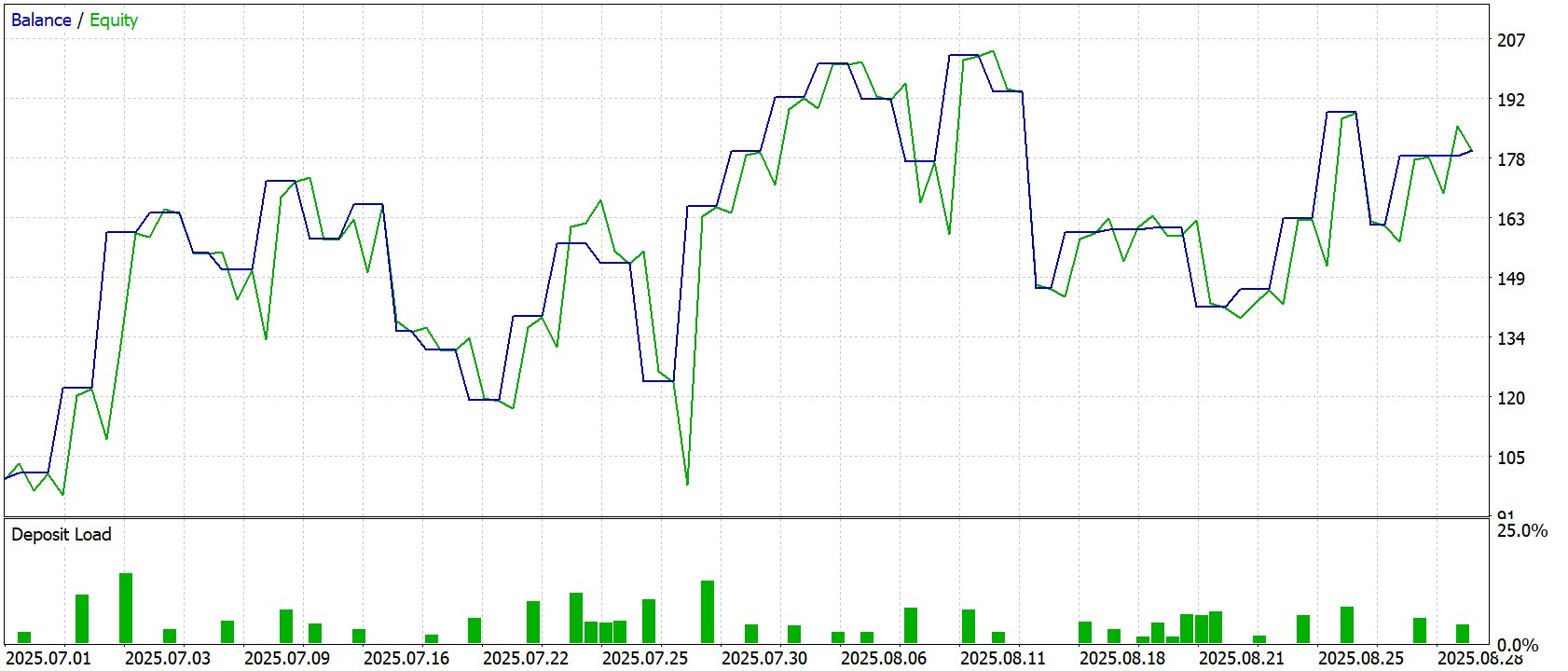
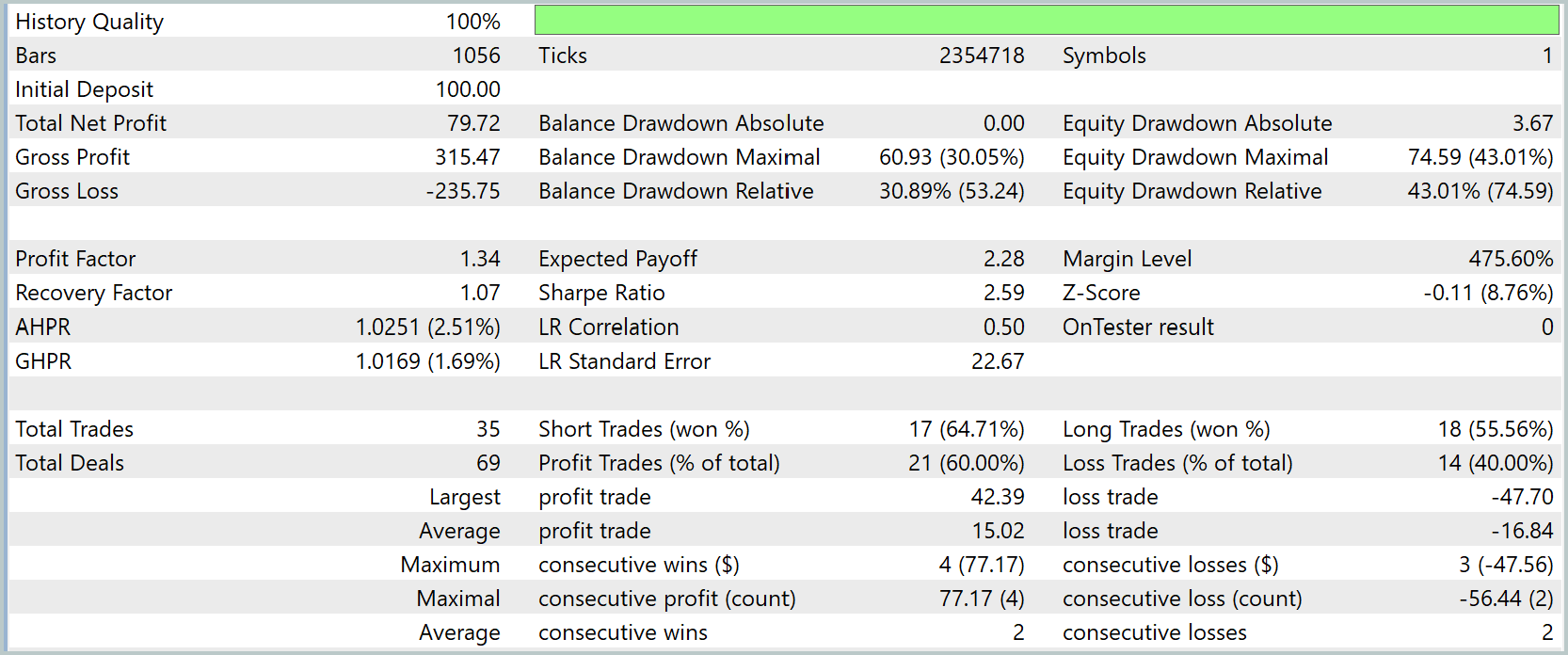
The model's test results demonstrate its training effectiveness and ability to adapt to real-world market conditions. The balance and equity chart shows that the model maintains steady capital growth despite market volatility. The Balance and Equity lines are virtually identical, indicating low capital drawdown and precise risk management.

An analysis of trade statistics confirms the strategy's effectiveness. The model generated a total net profit of 79.72 USD from an initial deposit of 100.0 USD. Total profit (Gross Profit) amounted to 315.47 USD, while total losses (Gross Loss) amounted to 235.75 USD, resulting in a Profit Factor of 1.34. This indicates that each dollar earned generated approximately 34 cents in net profit after losses, which is a respectable result for a real-time strategy.

It is important to note that the strategy exhibits moderate drawdowns: the maximum balance drawdown was 30.05%, while the maximum equity drawdown was 43.01%. At the same time, the Recovery Factor is 1.07, and the Sharpe Ratio reaches 2.59. All of this points to a good risk-return ratio.

The model demonstrated balanced performance with both short and long positions: 17 short trades with a win rate of 64.71% and 18 long trades with a win rate of 55.56%. A total of 69 trades were executed, of which 21 were profitable (60%) and 14 were unprofitable (40%).

Overall, the testing confirms that implementing the developed approaches and training on historical data, followed by real-time fine-tuning, enabled the model to respond effectively to market fluctuations and demonstrate high robustness and predictability in capital management.

Conclusion

We have completed the implementation of the approaches proposed by the authors of the ST-Expert framework and have successfully integrated them into the Extralonger framework. The resulting architecture allows for the simultaneous analysis of temporal and spatial data representations, combining global trends with local anomalies, which significantly improves forecasting accuracy and the robustness of strategies.

Special attention was paid to the reproducibility and determinism of all modules: from initialization and the forward pass to gradient calculation and weight updates. This approach ensures stable system behavior across various operating modes and simplifies the debugging of complex component interactions.

Test results based on real historical data demonstrated the model's effectiveness and its ability to adapt to various market conditions. The results confirm that combining global and local graph attention with temporal and spatial embeddings creates a solid foundation for practical application in the market, enabling models to adapt to changing conditions and deliver highly accurate forecasts while keeping computational costs under control.

Programs used in this article

#	Name	Type	Description
1	Study.mq5	Expert Advisor	Expert Advisor for offline model training
2	StudyOnline.mq5	Expert Advisor	Expert Advisor for online model training
3	Test.mq5	Expert Advisor	Expert Advisor for model testing
4	Trajectory.mqh	Class library	Structure describing the system state and model architecture
5	NeuroNet.mqh	Class library	Class library for building a neural network
6	NeuroNet.cl	Library	Code library for the OpenCL program

Translated from Russian by MetaQuotes Ltd.
Original article: https://www.mql5.com/ru/articles/19663

Attached files |

Download ZIP

MQL5.zip (3133.22 KB)

Warning: All rights to these materials are reserved by MetaQuotes Ltd. Copying or reprinting of these materials in whole or in part is prohibited.

This article was written by a user of the site and reflects their personal views. MetaQuotes Ltd is not responsible for the accuracy of the information presented, nor for any consequences resulting from the use of the solutions, strategies or recommendations described.