Unified Validation Pipeline Against Backtest Overfitting

Introduction

Every algorithmic trader eventually encounters a backtest that looks too good to be true. The equity curve is a near-perfect staircase climbing to the upper-right corner of the chart. The Sharpe ratio is exceptional. Drawdowns are shallow and brief.

The strategy then fails immediately upon going live.

This outcome is so common that it has earned its own vernacular in the quantitative research community. The culprit is almost always some form of overfitting: the algorithm has learned the historical noise of a specific dataset rather than any durable, forward-applicable market structure. What is less commonly understood is that overfitting is not a single phenomenon. It arrives through several distinct channels, each requiring a different countermeasure. A practitioner who deploys only one safeguard — the most common of which is a simple train/test split — remains exposed to the others.

This article examines three of the most rigorous tools available for combating overfitting in algorithmic strategy development: Validation-within-Validation (V-in-V), as articulated by Timothy Masters; Combinatorially Purged Cross-Validation (CPCV), developed by Marcos Lopez de Prado; and Combinatorially Symmetric Cross-Validation (CSCV), introduced by Bailey and Lopez de Prado. Each addresses a distinct failure mode. Together, they form a comprehensive defence against the most consequential forms of statistical self-deception in quantitative research.

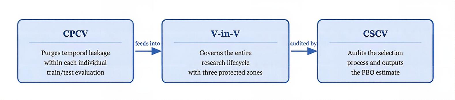
Figure 1. The unified research pipeline. CPCV purges temporal leakage inside individual evaluations; V-in-V governs the lifecycle; CSCV provides a final quantitative audit of the selection process

Part I: The Spaghetti-on-the-Wall Problem

The Brute-Force Temptation

The so-called spaghetti-on-the-wall approach refers to the practice of testing an enormous number of indicators, rules, and parameter combinations against a historical dataset in hopes that something will stick. Modern computing makes this approach trivially easy to execute and catastrophically easy to misinterpret.

The problem is also mathematical. If you conduct enough tests on any finite dataset, random chance alone will produce results that appear statistically significant. This is not a failure of intelligence or intent — it is a structural consequence of repeated hypothesis testing. Every additional test conducted on the same data raises the probability that the eventual winner is a statistical artifact rather than a genuine market edge.

The Primary Dangers

Data Snooping Bias. When the same historical data is used repeatedly to test different hypotheses, the probability that the eventual best performer is simply a lucky draw from randomness increases with each test. A strategy selected from ten thousand candidates on the same dataset carries very different probabilistic implications than one selected from five.

Curve-Fitting. An algorithm that has been allowed to optimise freely over historical data will, to some degree, fit the specific noise realisations of that particular price path. It will perform well on what has already happened precisely because it has learned to perform well on what has already happened. The noise of the past is not the signal of the future.

Researcher Degrees of Freedom. Even a researcher acting in complete good faith accumulates bias through the ordinary process of development. Every modelling decision that is informed, even indirectly, by observed performance on test data — feature selection, parameter bounds, rule structure — constitutes a degree of freedom that inflates the apparent significance of the final result. This form of contamination is invisible in any single decision but becomes severe in aggregate.

The spaghetti-on-the-wall approach is not inherently illegitimate. Broad exploratory search can surface genuine edges. The critical question is whether the researcher has applied safeguards rigorous enough to distinguish genuine edges from the statistical artifacts that such a search inevitably produces. Without all three layers of defense described here, it cannot.

Part II: Validation-within-Validation

The Hidden Flaw in Standard Walkforward Testing

The standard walkforward framework appears, on its surface, to be a complete solution. You train your strategy on historical data, test it on a subsequent out-of-sample period, declare success if it holds up, and move to live deployment. The framework is sound in principle. The problem is in the implementation.

Every time a researcher observes validation performance and uses that observation to make a modelling decision — adjusting a parameter, pruning a feature set, selecting among competing rule variants — the out-of-sample period becomes, in effect, part of the training set. The researcher's decision-making process has accessed that data.

This is what Masters terms the accumulation of researcher degrees of freedom, and it is arguably the most dangerous form of overfitting because it is invisible. The data partitions look clean on paper. The code is correctly structured. But the researcher's iterative responses to observed out-of-sample performance have introduced bias that standard partitioning cannot detect or correct.

The Three-Layer Architecture

Masters' solution is to create three strictly partitioned data pools, each serving a designated purpose and consuming the dataset's informational integrity at only that designated stage.

Total Historical Data
│
├── OUTER TRAINING SET (~60%)    ← Full exploratory search occurs here
│
├── INNER VALIDATION SET (~20%)  ← Candidate shortlisting occurs here
│                                   (Intentionally exposed to limited candidates)
│
└── FINAL TEST SET (~20%)        ← Opened exactly once, after full commitment

The Outer Training Set is where the full brute-force search is conducted. Thousands of rules, indicators, and parameter combinations are tested here. Every permutation test, regularisation pass, and exploratory analysis is performed within this boundary. The researcher may observe performance here freely, because this data is explicitly designated for exploration.

The Inner Validation Set is where candidate selection takes place. The shortlisted survivors from Phase 1 are exposed to this previously unseen data. Those that degrade severely are eliminated as likely overfit. This stage is used sparingly — the researcher commits to a small number of finalist configurations before exposing them here.

The Final Test Set is inviolable. It is opened exactly once, after the researcher has fully committed in writing to a single, final strategy configuration. The result of this single evaluation is the published performance figure. Any attempt to use this result to make further adjustments invalidates the test.

Figure 2. The three-layer data partition. Each zone serves one designated purpose. The Final Test Set is inviolable until a full written commitment to a single strategy has been made

Anchored Walkforward Expansion

The core problem it solves. A three-way data partition (60/20/20) is statistically sound in principle but practically punishing. On five years of daily data you might have 1,250 observations. A 20% Final Test Set gives you 250 bars — barely enough to estimate a Sharpe ratio with meaningful confidence intervals, and far too little to say anything about regime robustness. Shrinking the partition to get more test data just shifts the problem to the training set.

How it differs from standard rolling walkforward. Standard walkforward fixes the training window size and slides it forward. The training set rolls — old data drops off the left edge as new data is added to the right. This means the strategy is re-estimated from scratch each time on a different, equally-sized sample. Early market regimes are eventually discarded.

Anchored walkforward — a widely-used technique described clearly by Masters and others — fixes the start of the training set and expands it forward through time. The training set always begins at the same historical origin. Each successive window adds more data to it. The Final Test and Inner Validation windows advance in time but keep their proportional sizes relative to the total data consumed so far.

The individual Final Test results are not cherry-picked. They are evaluated as a single body of evidence. A strategy that holds its edge across the majority of test windows has demonstrated robustness across different market regimes and time periods — a much stronger claim than any single test-set result can provide.

Why it works — five interlocking reasons

1. Each Final Test window is genuinely out-of-sample. The strategy configuration that faces each test window was committed to before that window was opened. The temporal boundary is strict.
2. The test results are substantially independent. Because each Final Test window covers a different, non-overlapping slice of calendar time, the individual test results are largely independent observations of market performance — though the overlapping training data creates some serial correlation in parameter estimates that should be borne in mind when aggregating results.
3. Anchoring accumulates rather than discards information. Rolling walkforward throws away early data when the window advances. Anchoring keeps all historical data in the training set as the window grows.
4. Multiple test results reveal regime sensitivity. A strategy that holds its edge across all test windows has proven itself across whatever market conditions occurred across the full historical span. A strategy that performs well in some windows and fails in others is revealing genuine regime sensitivity — a finding a single test window would completely obscure.
5. The three-layer integrity is preserved in every window. Each window maintains its own Inner Validation boundary. The lifecycle discipline that makes V-in-V meaningful is not relaxed — it is applied repeatedly.

The catch — and why it matters less than it appears

The individual test windows are not fully independent. Later windows share most of their training data with earlier ones, creating serial correlation in the parameter estimates used to generate each window's result. The test results should therefore be evaluated qualitatively — as a body of evidence asking whether the edge persists and whether its magnitude is roughly consistent — rather than combined into a single pooled statistic with a falsely inflated sample size.

Figure 3. Standard walkforward expansion

Figure 4. Anchored walkforward expansion — three windows showing training set growing while Inner Validation and Final Test shift forward

Implementation

The code below shows how to structure the full V-in-V three-layer pipeline using PurgedWalkForwardCV. The outer training data is what you pass to PurgedWalkForwardCV; the inner validation and final test sets are manually held out beforehand.

import numpy as np
import pandas as pd
from sklearn.base import clone

from cross_validation import PurgedWalkForwardCV

def vin_v_anchored_walkforward(
    X: pd.DataFrame,
    y: pd.Series,
    t1: pd.Series,
    estimator,
    n_splits: int = 5,
    inner_val_pct: float = 0.20,
    final_test_pct: float = 0.20,
    pct_embargo: float = 0.01,
    scorer=None,
) -> dict:
    """
    Three-layer V-in-V pipeline with anchored expanding-window walkforward.

    Data is partitioned once, strictly in temporal order:
        [─── Outer Training (60%) ───][─ Inner Val (20%) ─][─ Final Test (20%) ─]

    The outer training set is further split by PurgedWalkForwardCV into
    n_splits expanding windows, each producing its own purged train/test pair.
    The inner validation set is touched only for shortlisting; the final test
    set is opened exactly once after a written commitment to a single config.

    Parameters
    ----------
    X, y, t1 : aligned DataFrame, Series, Series
    estimator  : sklearn-compatible estimator
    n_splits   : number of anchored walkforward windows within outer training
    inner_val_pct, final_test_pct : fractions of total data reserved
    pct_embargo : embargo fraction passed to PurgedWalkForwardCV
    scorer     : callable(y_true, y_pred) -> float, or None (returns raw preds)

    Returns
    -------
    dict with keys:
        outer_scores    – per-window score within outer training
        inner_val_score – score on the inner validation set (shortlisting only)
        final_test_score– score on the final test set (opened once, at the end)
        outer_cv        – the fitted PurgedWalkForwardCV object
    """
    n = len(X)

    # ── 1. Partition the data into three zones ───────────────────────────────
    outer_end   = int(n * (1.0 - inner_val_pct - final_test_pct))
    val_end     = int(n * (1.0 - final_test_pct))

    X_outer,     y_outer,     t1_outer     = X.iloc[:outer_end],  y.iloc[:outer_end],  t1.iloc[:outer_end]
    X_inner_val, y_inner_val, t1_inner_val = X.iloc[outer_end:val_end], y.iloc[outer_end:val_end], t1.iloc[outer_end:val_end]
    X_final,     y_final                   = X.iloc[val_end:],    y.iloc[val_end:]

    # ── 2. Phase 1 — exhaustive search within outer training ─────────────────
    # PurgedWalkForwardCV(expanding_window=True) anchors the start at index 0
    # and grows the training window forward — this IS anchored walkforward.
    outer_cv = PurgedWalkForwardCV(
        n_splits=n_splits,
        t1=t1_outer,
        pct_embargo=pct_embargo,
        expanding_window=True,   # ← anchored, not rolling
    )

    outer_scores = []
    outer_models = []

    for train_idx, test_idx in outer_cv.split(X_outer, y_outer):
        model = clone(estimator)
        model.fit(X_outer.iloc[train_idx], y_outer.iloc[train_idx])
        preds = model.predict(X_outer.iloc[test_idx])

        score = scorer(y_outer.iloc[test_idx], preds) if scorer else None
        outer_scores.append(score)
        outer_models.append(model)

    # At this point the researcher reviews outer_scores, shortlists candidates,
    # and selects a small number of finalist configurations. The inner
    # validation set is NOT touched yet.

    # ── 3. Phase 2 — shortlist on inner validation (sparingly) ───────────────
    # Only finalist models are exposed here. This set must not be used
    # to refine parameters — observation terminates candidate selection.
    finalist_model = outer_models[-1]   # placeholder: researcher selects this
    val_preds      = finalist_model.predict(X_inner_val)
    inner_val_score = scorer(y_inner_val, val_preds) if scorer else None

    # ── 4. Phase 3 — final test (opened exactly once) ────────────────────────
    # The researcher commits in writing to finalist_model before this line.
    # Any adjustment after seeing this result invalidates the test.
    final_preds      = finalist_model.predict(X_final)
    final_test_score = scorer(y_final, final_preds) if scorer else None

    return {
        "outer_scores":     outer_scores,
        "inner_val_score":  inner_val_score,
        "final_test_score": final_test_score,
        "outer_cv":         outer_cv,
    }

# ── Example usage ─────────────────────────────────────────────────────────
if __name__ == "__main__":
    from sklearn.ensemble import RandomForestClassifier
    from sklearn.metrics import accuracy_score

    dates  = pd.date_range("2018-01-01", periods=1000, freq="B")
    X_demo = pd.DataFrame(np.random.randn(1000, 5), index=dates)
    y_demo = pd.Series(np.random.randint(0, 2, 1000), index=dates)
    t1_demo = pd.Series(dates + pd.Timedelta(days=5), index=dates)

    results = vin_v_anchored_walkforward(
        X=X_demo, y=y_demo, t1=t1_demo,
        estimator=RandomForestClassifier(n_estimators=50, random_state=42),
        n_splits=5,
        scorer=accuracy_score,
    )

    print("Outer window scores:", results["outer_scores"])
    print("Inner validation:  ", results["inner_val_score"])
    print("Final test score:  ", results["final_test_score"])

Part III: Combinatorially Purged Cross-Validation

The Problem CPCV Was Built to Solve

Validation-within-Validation assumes that the individual evaluations conducted within the Outer Training Set are themselves clean. It governs the lifecycle of the research process but does not inspect the internal validity of each train/test evaluation.

This is the problem CPCV, developed by Marcos Lopez de Prado in Advances in Financial Machine Learning, was built to solve. The contamination it addresses is not behavioural, it is structural, embedded in the statistical properties of financial time series themselves.

Why Financial Data Is Different

Standard k-fold cross-validation — the workhorse of machine learning — assumes that observations are independently and identically distributed. Financial time series violate this assumption profoundly and in multiple overlapping ways.

Consider a feature set that includes a 20-day moving average. The observation computed on Day 21 shares 19 of its 20 underlying data points with the observation computed on Day 20. If these two observations are assigned to different folds — one to training, one to testing — the test fold has effectively seen nearly all of the training data that produced the corresponding training observation. The boundary between training and test is an illusion.

This problem is compounded by the labelling process. In financial machine learning, observations are typically labelled based on the outcome of a future holding period. A label formed by the return over the next 10 days creates a dependency between the labelled observation and the 10 subsequent price bars. Those subsequent bars will almost certainly appear as feature inputs elsewhere in the dataset, creating a leakage channel that standard purging does not address.

Figure 5 illustrates the k train/test splits carried out by a k-fold CV, where k = 5. In this scheme:

1. The dataset is partitioned into k subsets.
2. For i = 1,…,k:
   • (a) The ML algorithm is trained on all subsets excluding i.
   • (b) The fitted ML algorithm is tested on i.

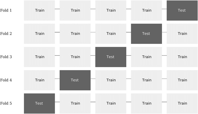
Figure 5. Train/test splits in a 5-fold CV scheme

The Two Purging Mechanisms

Purging. After a test fold is assigned, CPCV removes from the training set any observation whose label formation window overlaps in time with the test period. This is not simply a matter of separating time periods — the purge must account for the specific horizon over which each observation's label was computed.

Embargoing. A buffer of observations immediately following the test fold is also removed from training. Features calculated on these post-test observations may look backward into the test period, creating a reverse leakage channel. The embargo window is sized to the longest feature lookback in the feature set.

Figure 6. Purge of train observations pre-test and embargo of post-test train observations

The Combinatorial Paths

Beyond purging and embargoing, CPCV introduces a structural improvement over standard k-fold validation. Rather than a single train/test split, it generates all possible combinations of fold assignments. These splits are then recombined into complete backtest paths.

Consider T observations partitioned into N groups without shuffling, where groups n = 1, ... , N − 1 are of size ⌊T∕N⌋, the Nth group is of size T − ⌊T∕N⌋ (N − 1), and ⌊.⌋ is the floor or integer function. For a testing set of size k groups, the number of possible training/testing splits is

Since each combination involves k tested groups, the total number of tested groups is . And since we have computed all possible combinations, these tested groups are uniformly distributed across all N (each group belongs to the same number of training and testing sets). The implication is that from k-sized testing sets on N groups we can backtest a total number of paths 𝜑 [N, k],

... There are C(6, 4) = 15 splits, indexed as S1, … ,S15. For each split, the figure ... leaves unmarked the groups that form the training set. Each group forms part of 𝜑 [6, 2] = 5 testing sets, therefore this train/test split scheme allows us to compute 5 backtest paths.

Figure 7 shows the assignment of each tested group to one backtest path. For example, path 1 is the result of combining the forecasts from (G1, S1), (G2, S1), (G3, S2), (G4, S3), (G5, S4) and (G6, S5). Path 2 is the result of combining forecasts from (G1, S2), (G2, S6), (G3, S6), (G4, S7), (G5, S8) and (G6, S9), and so on.

These paths are generated by training the classifier on a portion 𝜃 = 1 − k∕N of the data for each combination. Although it is theoretically possible to train on a portion 𝜃 < 1∕2, in practice we will assume that k ≤ N∕2. The portion of data in the training set 𝜃 increases with N → T but it decreases with k → N∕2. The number of paths 𝜑 [N, k] increases with N → T and with k → N∕2. In the limit, the largest number of paths is achieved by setting N = T and k = N∕2 = T∕2, at the expense of training the classifier on only half of the data for each combination (𝜃 = 1∕2).

Figure 7. Assignment of testing groups to each of the 5 paths

Lopez de Prado, 2018, p. 164-165

With N=6 groups and k=2 test groups, each path stitches together the out-of-sample segments from a subset of splits to cover the full timeline exactly once, yielding C(6,2) × k / N = 5 complete paths. It is these paths — not the individual splits — that are the correct basis for computing Sharpe ratios and assessing distributional robustness.

This distribution is itself informative. A strategy with a narrow, positive distribution of path outcomes across all combinatorial fold assignments has demonstrated robustness across many different temporal configurations. A strategy whose performance varies dramatically across paths is fragile, regardless of its mean performance.

Figure 8: Bar chart of 5 CPCV path Sharpe ratios side-by-side for a robust strategy and a fragile strategy

Implementation

import numpy as np
import pandas as pd
from sklearn.ensemble import RandomForestClassifier

from combinatorial import CombinatorialPurgedCV, CPCVAnalyzer, optimal_folds_number

# ── 1. Configure the CV generator ────────────────────────────────────────
# Use optimal_folds_number to find N and k that meet your targets.
# Here: aim for ~600 obs in each training set and 5 backtest paths.
n_folds, n_test_folds = optimal_folds_number(
    n_observations=1000,
    target_train_size=600,
    target_n_test_paths=5,
)
print(f"n_folds={n_folds}, n_test_folds={n_test_folds}")

cv = CombinatorialPurgedCV(
    n_folds=n_folds,
    n_test_folds=n_test_folds,
    t1=t1_outer,          # pd.Series: index=event start, values=event end
    pct_embargo=0.01,     # removes 1% of obs after each test block
)

print(cv.summary(X_outer))
# Number of Observations      1000
# Total Number of Folds          6
# Number of Test Folds           2
# Number of Test Paths           5
# Number of Training Combinations 15

# ── 2. Fit and predict across all combinatorial splits ───────────────────
# CPCVAnalyzer handles the parallel execution and path recombination.
analyzer = CPCVAnalyzer(
    estimator=RandomForestClassifier(n_estimators=100, random_state=42),
    cv_gen=cv,
    close_prices=close_prices,   # pd.Series of price for MtM Sharpe calculation
)

recombined_preds = analyzer.fit_predict(X_outer, y_outer)


# ── 3. Inspect the distribution of path Sharpe ratios ───────────────────
# Each path is an independent backtest covering the full timeline once.
# A tight, positive distribution signals robustness.
metrics = analyzer.get_distribution_metrics(primary_sides=sides)

path_sharpes = metrics.xs("binary", level="method")["mtm_sharpe"]
print("Path Sharpe ratios:")
print(path_sharpes.to_string())
print(f"Mean: {path_sharpes.mean():.3f}  Std: {path_sharpes.std():.3f}")


# ── 4. Visualise train/test fold assignments ─────────────────────────────
# Run split() fully first so index_train_test_ is complete.
_ = [s for s in cv.split(X_outer)]   # exhaust generator
fig = cv.plot_train_test_folds()
fig.show()

Part IV: Combinatorially Symmetric Cross-Validation

From Protection to Measurement

Where V-in-V and CPCV are protective mechanisms — they reduce overfitting by structuring the research process and purging data leakage — CSCV is primarily a diagnostic and measurement tool. Its output is a single number: the Probability of Backtest Overfitting (PBO).

CSCV was introduced by David Bailey and Marcos Lopez de Prado as a method for quantifying the degree to which a strategy selection process is producing results attributable to in-sample optimisation rather than genuine out-of-sample predictive power. The PBO is a falsifiable, communicable claim, not a qualitative judgement. It can be applied at any stage of the research pipeline where a candidate set exists — not exclusively after the V-in-V shortlisting phase — making it a flexible audit instrument.

The Mechanics

The procedure begins by dividing the historical data into S equal subsets, typically between 8 and 16. All C(S, S/2) ways to split those subsets into a training half and a test half are then generated. For each split, the strategy with the best in-sample performance is identified. Its rank among all strategies on the out-of-sample half of that same split is then recorded.

Figure 9. CSCV Step 1: data is divided into S equal subsets. All C(S, S/2) ways of assigning half to in-sample (IS, green) and half to out-of-sample (OOS, red) are then enumerated

Figure 10. CSCV Step 2: for each split, the best in-sample (IS) strategy is identified (S3★), then its rank in the out-of-sample (OOS) half is recorded. Here it ranks 4th out of 6 — below the median — contributing to the PBO count.

Figure 11. CSCV Step 3: the proportion of splits where the best in-sample strategy ranked below the median out-of-sample is the PBO estimate. A PBO of 0.38 suggests meaningful selection bias in the research process

Figure 12. PBO interpretation. A PBO near 0 indicates the selection process reliably identifies genuine out-of-sample leaders. A PBO near 0.5 indicates the best in-sample strategy is essentially randomly ranked out-of-sample. The threshold for "acceptable" varies by context and candidate set size — it is a rule of thumb, not a formal statistical boundary

What CSCV Does Not Do

CSCV does not fix overfitting. It does not purge temporal leakage, does not control researcher degrees of freedom, and does not structure the research lifecycle. A high PBO score tells you that your selection process is unreliable — it does not tell you how to make it reliable.

CSCV is most powerful when used as a final audit: run after your candidate shortlist has been assembled using the V-in-V framework, it produces a PBO score for the selection process as a whole. A low PBO score provides a quantitative, communicable assurance that the selection process was generating signal rather than noise. However, because CSCV operates on any collection of strategy trial results, it can equally be applied at earlier stages, for instance to audit the candidate generation process inside the Outer Training Set.

[!] Note on thresholds: The original Bailey & Lopez de Prado paper does not establish a universal PBO threshold for "acceptable" results. Values such as 0.1 or 0.2 are informal rules of thumb that depend on the number of candidates tested, the length of the historical sample, and the practitioner's tolerance for selection risk. They should not be treated as formal statistical criteria.

Implementation

CSCV reuses CombinatorialPurgedCV directly. Because CSCV treats all subsets symmetrically — there is no temporal arrow between in-sample and out-of-sample halves — set pct_embargo=0.0 and n_test_folds=n_folds//2. This produces exactly the C(S, S/2) symmetric splits described above.

"""
Probability of Backtest Overfitting (PBO) — Bailey & Lopez de Prado (2014).

Uses CombinatorialPurgedCV with pct_embargo=0.0 and n_test_folds=n_folds//2
to generate the C(S, S/2) symmetric IS/OOS splits required by CSCV.
"""
from math import comb
from typing import Callable, Dict, List

import numpy as np
import pandas as pd
from scipy.stats import norm

from combinatorial import CombinatorialPurgedCV

def compute_pbo(
    returns_matrix: pd.DataFrame,
    t1: pd.Series,
    n_folds: int = 8,
    metric: Callable = None,
) -> Dict:
    """
    Compute the Probability of Backtest Overfitting (PBO).

    Parameters
    ----------
    returns_matrix : pd.DataFrame, shape (T, N)
        Columns are candidate strategies; rows are time-ordered observations.
        Values should be per-period returns (or any scalar performance measure
        that is comparable across strategies at a given time step).

    t1 : pd.Series
        Event end-times aligned with returns_matrix.index. Because CSCV is
        symmetric (no temporal arrow), pct_embargo is set to 0.0, so t1 is
        used only to satisfy the CombinatorialPurgedCV interface — you may
        pass t1 = pd.Series(index, index=index) as a neutral value.

    n_folds : int, default=8
        Number of equal subsets S. Must be even. C(S, S/2) splits are
        generated. Bailey & Lopez de Prado recommend 8–16.

    metric : callable(returns: pd.Series) -> float, optional
        Aggregates a column of returns into a scalar performance measure.
        Defaults to the Sharpe ratio (mean/std).

    Returns
    -------
    dict with keys:
        pbo          – float in [0, 1]: estimated probability of overfitting
        n_splits     – total number of IS/OOS splits evaluated (= C(S, S/2))
        below_median – number of splits where best-IS ranked below OOS median
        oos_ranks    – list of normalised OOS ranks for the best-IS strategy
                       (0 = best OOS, 1 = worst OOS)
        logit_sr     – logit-transformed OOS score (if in (0,1)) for best-IS strategy per split
    """
    if n_folds % 2 != 0:
        raise ValueError(f"n_folds must be even for symmetric CSCV; got {n_folds}.")

    n_test_folds = n_folds // 2          # ← symmetric split: half IS, half OOS

    if metric is None:
        def metric(r: pd.Series) -> float:
            """Sharpe ratio."""
            return r.mean() / r.std(ddof=1) if r.std() > 0 else 0.0

    # ── Build the CSCV generator ──────────────────────────────────────────
    # pct_embargo=0.0  → no embargo (CSCV is symmetric, not temporal)
    # n_test_folds=n_folds//2 → exactly half the folds form the OOS set
    cv = CombinatorialPurgedCV(
        n_folds=n_folds,
        n_test_folds=n_test_folds,   # = n_folds // 2
        t1=t1,
        pct_embargo=0.0,             # ← required for symmetric CSCV
    )

    n_strategies = returns_matrix.shape[1]
    below_median = 0
    oos_ranks    = []
    logit_sr     = []

    # ── Iterate over all C(n_folds, n_folds//2) symmetric splits ────────
    for train_idx, test_idx_list in cv.split(returns_matrix):
        test_idx = np.concatenate(test_idx_list)

        # IS half: compute metric for every strategy
        is_scores = returns_matrix.iloc[train_idx].apply(metric, axis=0)

        # OOS half: compute metric for every strategy
        oos_scores = returns_matrix.iloc[test_idx].apply(metric, axis=0)

        # Best IS strategy
        best_is_col = is_scores.idxmax()

        # Rank of that strategy OOS (0-based; 0 = best OOS performer)
        oos_sorted = oos_scores.rank(ascending=False)   # rank 1 = best
        oos_rank   = oos_sorted[best_is_col]               # 1-indexed

        # Normalise rank to [0, 1]: 0 = best OOS, 1 = worst OOS
        norm_rank = (oos_rank - 1) / (n_strategies - 1) if n_strategies > 1 else 0.0
        oos_ranks.append(float(norm_rank))

        # Below median? (norm_rank > 0.5 means worse than median)
        if norm_rank > 0.5:
            below_median += 1

        # Logit-transformed OOS score (if in (0,1)) for the best-IS strategy
        oos_sr = float(oos_scores[best_is_col])
        logit_sr.append(np.log(oos_sr / (1 - oos_sr)) if 0 < oos_sr < 1 else np.nan)

    n_splits = cv.n_splits
    pbo      = below_median / n_splits

    return {
        "pbo":          pbo,
        "n_splits":     n_splits,
        "below_median": below_median,
        "oos_ranks":    oos_ranks,
        "logit_sr":     [v for v in logit_sr if not np.isnan(v)],
    }

# ── Example usage ─────────────────────────────────────────────────────────
if __name__ == "__main__":
    # Simulate 50 strategy return streams over 500 time steps
    rng     = np.random.default_rng(42)
    dates   = pd.date_range("2020-01-01", periods=500, freq="B")
    returns = pd.DataFrame(
        rng.normal(0.0001, 0.01, size=(500, 50)),
        index=dates,
        columns=[f"strategy_{i}" for i in range(50)],
    )

    # Neutral t1: event start == event end (no label horizon, no purging effect)
    t1_neutral = pd.Series(dates, index=dates)

    result = compute_pbo(
        returns_matrix=returns,
        t1=t1_neutral,
        n_folds=8,      # → n_test_folds=4, C(8,4)=70 splits
    )

    print(f"PBO  : {result['pbo']:.3f}")
    print(f"Splits evaluated : {result['n_splits']}")
    print(f"Below median (IS best → OOS below median): {result['below_median']}")

    # Interpret: if returns are pure noise, PBO ≈ 0.5
    # A strategy with genuine edge should push PBO toward 0

Part V: A Unified Pipeline

Mapping the Techniques to the Research Stages

The relationship between these three techniques becomes clear when they are mapped against the phases of the V-in-V research lifecycle. They do not compete. They occupy different positions in the pipeline and protect against different threats.

Technique	Stage in Pipeline	Threat Addressed	Output
CPCV	Inside Outer Training (Phase 1)	Temporal leakage within each train/test evaluation	Clean per-evaluation performance paths
V-in-V	Governs the entire lifecycle	Researcher degrees of freedom accumulated across iterations	Lifecycle structure with three protected zones
CSCV	After candidate shortlisting (Phase 2), or at any stage where a candidate set exists	Selection bias over the candidate set	PBO — a falsifiable probability estimate

Are They Solving the Same Problem?

The three techniques are related in that they all exist because naive train/test splits produce optimistic performance estimates in financial data. But they address genuinely different mechanisms of that shared problem.

Validation-within-Validation addresses behavioural contamination accumulated across the development lifecycle by a human researcher making iterative modelling decisions. This contamination is introduced by the researcher and would not exist if a single, non-iterative strategy selection were made at the outset.

Combinatorially Purged Cross-Validation addresses structural contamination embedded in the temporal dependence of financial observations. This contamination exists in the data itself and would persist even if the researcher made no iterative decisions whatsoever — it is a mathematical property of financial time series.

Combinatorially Symmetric Cross-Validation quantifies the probability that the selection process as a whole produced an overfit result, providing a falsifiable, communicable claim about the reliability of the chosen strategy that neither of the other two techniques produces.

Running CPCV without V-in-V's structural discipline produces clean individual evaluations but leaves researcher degrees of freedom uncontrolled. A developer could run CPCV through fifty iterations of strategy refinement, observe each result, and allow each observation to influence the next modelling decision. Each individual evaluation would be clean, but the research process as a whole would be contaminated.

Conversely, running V-in-V without CPCV inside Phase 1 preserves the Final Test Set perfectly but may produce a candidate from Phase 1 that was selected on the basis of leakage-inflated evaluations. The three-layer structure protects the Final Test Set, but the candidacy mechanism that feeds it is compromised.

Omitting CSCV means the practitioner has no quantitative estimate of how reliable the selection process was. They have protected themselves against known leakage channels but have no auditable, communicable claim about the probability that the selected strategy is a genuine edge rather than a lucky draw.

Which Technique Is Most Important?

If forced to prioritise by the severity of the bias introduced when each is omitted in isolation, the following ordering is a reasonable starting point — though practitioners should note this is an editorial judgement rather than a settled empirical finding, and the relative importance of each technique will vary with dataset length, feature complexity, and the intensity of the research programme.

1. CPCV — Non-negotiable for financial time series. Standard k-fold cross-validation is not merely suboptimal for financial data; it is structurally wrong. The i.i.d. assumption it requires is violated by virtually every financial feature set. Temporal leakage inflates performance estimates in a way that cannot be corrected after the fact.

2. V-in-V — Non-negotiable for any iterative research programme. In practice, every serious strategy development effort involves weeks or months of iterative refinement. Without V-in-V's structural discipline, every observation of out-of-sample performance that influences a subsequent decision constitutes unaccounted researcher degrees of freedom. In a long, intensive research programme this accumulated effect may dwarf any single source of data leakage — making a strong argument that V-in-V can be equally or more important than CPCV in practice.

3. CSCV — Uniquely valuable for communicating findings. Its quantitative PBO output provides something the other two techniques cannot: a single, defensible number that summarises the reliability of the entire selection process. This makes it particularly valuable in institutional contexts where research must be reviewed, peer-validated, or communicated to stakeholders who cannot inspect the full methodology.

Conclusion

The spaghetti-on-the-wall approach to strategy discovery does not have to be intellectually disreputable. Broad exploratory search over large indicator spaces can surface genuine market edges, provided the researcher has constructed a validation infrastructure rigorous enough to separate genuine signal from the statistical noise that brute-force search inevitably produces.

No single technique is sufficient. V-in-V, CPCV, and CSCV each address a distinct failure mode, operate at a different stage of the research pipeline, and provide a different form of protection or measurement. Deploying one without the others leaves meaningful attack surface open.

CPCV ensures that every train/test evaluation within the exploratory phase is free of temporal information leakage. V-in-V ensures that the research lifecycle as a whole does not accumulate researcher degrees of freedom that inflate the apparent significance of the final strategy selection. CSCV provides a quantitative, auditable estimate of the probability that the selection process itself produced a genuine edge rather than an optimised artifact of the available data.

Together, these three techniques transform the Sharpe ratio (or any other performance metric) of a backtest from a number that reflects what a researcher hoped to find into a number that represents what the strategy is actually likely to deliver.

Code Reference

The implementation examples throughout this article draw on five files. The table below summarises their roles and relationships.

File	Purpose	Key Contents	Dependencies
cross_validation.py	Core purging and walk-forward CV primitives. Foundation for all higher-level components.	ml_get_train_times — vectorised event-based purging; PurgedKFold — standard purged k-fold; PurgedWalkForwardCV — anchored (expanding) or rolling walk-forward with purging and embargo; ml_cross_val_score — single-metric CV runner; analyze_cross_val_scores — multi-metric CV runner with confusion matrix breakdown.	None (base module)
combinatorial.py	Combinatorially Purged Cross-Validation engine. Generates all C(N,k) train/test splits, recombines them into φ[N,k] complete backtest paths, and computes the full distribution of path-level performance metrics.	CombinatorialPurgedCV — sklearn-compatible CV generator with purging, embargo, path recombination, and fold visualisation; CPCVAnalyzer — parallel fit/predict and MtM Sharpe distribution across all paths; optimal_folds_number — finds the (N, k) pair that best matches target training size and path count.	cross_validation.py (imports ml_get_train_times)
anchored_walkforward.py	Implements the full three-layer V-in-V research lifecycle using an anchored expanding window. Enforces strict separation of the outer training, inner validation, and final test zones.	vin_v_anchored_walkforward — partitions data into three temporal zones, runs PurgedWalkForwardCV(expanding_window=True) within the outer zone, exposes the inner validation set only for shortlisting, and opens the final test set exactly once after a written commitment.	cross_validation.py
cpcv_usage.py	Usage example showing how to configure and run CPCV within the outer training zone of a V-in-V pipeline, inspect the Sharpe distribution across paths, and correctly invoke the fold visualisation methods.	Demonstrates optimal_folds_number, CombinatorialPurgedCV.summary, CPCVAnalyzer.fit_predict, get_distribution_metrics, and the correct call order for plot_train_test_index and plot_train_test_folds.	combinatorial.py
pbo.py	Computes the Probability of Backtest Overfitting (PBO) using CombinatorialPurgedCV configured for symmetric CSCV splits. Accepts any matrix of strategy returns and a performance metric, and returns the PBO estimate along with per-split OOS rank diagnostics.	compute_pbo — sets pct_embargo=0.0 and n_test_folds=n_folds//2 to produce the C(S, S/2) symmetric splits required by CSCV; identifies the best in-sample strategy per split; records its normalised out-of-sample rank; and aggregates the proportion of splits where it ranked below the OOS median.	combinatorial.py

Further Reading

• Masters, T. (1995). Advanced Algorithms for Neural Networks. John Wiley & Sons.
• Masters, T. (2013). Permutation and Randomization Tests for Trading System Development. Self-published.
• Lopez de Prado, M. (2018). Advances in Financial Machine Learning. John Wiley & Sons.
• Bailey, D. H., & Lopez de Prado, M. (2014). The Deflated Sharpe Ratio: Correcting for Selection Bias, Backtest Overfitting and Non-Normality. Journal of Portfolio Management.
• Bailey, D. H., Borwein, J., Lopez de Prado, M., & Zhu, Q. J. (2014). Pseudo-Mathematics and Financial Charlatanism: The Effects of Backtest Overfitting on Out-of-Sample Performance. Notices of the AMS.
• White, H. (2000). A Reality Check for Data Snooping. Econometrica, 68(5), 1097–1126.