Mathematics in trading: Sharpe and Sortino ratios

Return on investments is the most obvious indicator which investors and novice traders use for the analysis of trading efficiency. Professional traders use more reliable tools to analyze strategies, such as Sharpe and Sortino ratios, among others. In this article, we will consider simple examples to understand how these ratios are calculated. The specifics of evaluation of trading strategies were earlier considered in the article "Mathematics in trading. How to estimate trading results". It is recommended that you read the article to refresh the knowledge or to learn something new.

Sharpe ratio

Experienced investors and traders often trade multiple strategies and invest in different assets in an effort to get consistent results. This is one of the concepts of smart investment which implies the creation of an investment portfolio. Each portfolio of securities/strategies has its own risk and return parameters, which should somehow be compared.

One of the most referenced tools for such comparison is the Sharpe ratio, which was developed in 1966, by Nobel laureate William F. Sharpe. The ratio calculation uses basic performance metrics, including the average rate of return, standard deviation of return and risk-free return.

The disadvantage of the Sharpe ratio is that the source data used for the analysis must be normally distributed. In other words, the return distribution graph should be symmetrical, and it should not have sharp peaks or falls.

The Sharpe ratio is calculated using the following formula:

Sharpe Ratio = (Return - RiskFree)/Std

Where:

• Return — the average rate of return for a certain period. For example, for a month, quarter, year, etc.
  
• RiskFree — risk-free return rate for the same period. Traditionally, these include bank deposits, bonds and other minimum-risk assets with 100% reliability.
  
• Std — standard deviation of the portfolio returns for the same period. The greater the returns deviate from the expected value, the higher the risk and the volatility experienced by the trader's account or portfolio assets.
  

Return

The return is calculated as a change in the value of assets for a certain interval. Return values are used for the same time period for which the Sharpe ratio is calculated. Usually, the annual Sharpe ratio is considered, but it is also possible to calculate quarterly, monthly or even daily values. The return is calculated by the following formula:

Return[i] = (Close[i]-Close[i-1])/Close[i-1]

Where:

• Return[i] — return for the i interval;
• Close[i] — the value of the assets at the end of the i-th interval;
• Close[i-1] — the value of the assets at the end of the previous interval.

In other words, the return can be written as a relative change in the asset value for the selected period:

Return[i] = Delta[i]/Previous

Where:

• Delta[i] = (Close[i]-Close[i-1]) — absolute change in the asset value for the selected period;
• Previous = Close[i-1] — the value of assets at the end of the previous interval.
  

To calculate the Sharpe ratio for a period of one year using daily values, we should use the return values for each day during the year and calculate the average daily return as a sum of returns divided by the number of days in the calculation. 

Return = Sum(Return[i])/N

where N is the number of days.

Risk-free return

The concept of risk-free return is conditional, since there is always a risk. Since the Sharpe ratio is used for comparing different strategies/portfolios in the same time intervals, the zero risk-free return can be used on the formula. That is,

RiskFree = 0

Standard deviation or return

The standard deviation shows how random variables deviate from a mean value. First, the average return value is calculated, then the squared deviations of returns from the average value are summed up. The resulting sum is divided by the number of returns to obtain dispersion. Square root of dispersion is the standard deviation.

D = Sum((Return - Return[i])^2 )/N

STD = SQRT(D)

Example of standard deviation calculation is provided in the previously mentioned article.

Calculating the Sharpe ratio on any timeframe and converting it to an annual value

The Sharpe ratio calculation method has not changed since 1966. The variable received its modern name after this calculation methodology was widely recognized. At that time, fund and portfolio performance evaluations were based on returns received for several years. Later, calculations were made on monthly data, while the resulting Sharpe ratio was mapped into an annual value. This method enables the comparison of two funds, portfolios or strategies.

The Sharpe Ratio can be easily scaled from different periods and timeframes into an annual value. This is done by multiplying the resulting value by the square root of the ratio of the annual interval to the current one. Let us consider the following example.

Suppose we have calculated the Sharpe ratio using daily return values — SharpeDaily. The result should be converted to the annual value SharpeAnnual. The annual ratio is proportional to the square root of the ratio of periods, i.e. how many daily intervals fit into one year. Since there are 252 working days in one year, the daily return-based Sharpe ratio should be multiplied by the square root of 252. This will be the annual Sharpe ratio:

SharpeAnnual = SQRT(252)*SharpeDaily // 252 working days in a year

If the value is calculated based on the H1 timeframe, we use the same principle — first convert SharpeHourly to SharpeDaily, and then calculate the annual Sharpe ratio. One D1 bar includes 24 H1 bars, which is why the formula will be as follows:

SharpeDaily = SQRT(24)*SharpeHourly   // 24 hours fit into D1

Not all financial instruments are traded 24 hours a day. But this is not important when evaluating trading strategies in the tester for the same financial instrument, since comparison is performed for the same testing interval and the same timeframe.

Evaluating strategies using the Sharpe ratio

Depending on the strategy/portfolio performance, the Sharpe Ratio can have different values, even negative ones. The conversion of the Sharpe ratio to an annual value enables its interpretation in a classical way:

Value	Meaning	Description
Sharpe Ratio < 0	Bad	The strategy is unprofitable
0 < Sharpe Ratio  < 1.0	Undefined	The risk does not pay off. Such strategies can be considered when there are no alternatives
Sharpe Ratio ≥ 1.0	Good	If the Sharpe ratio is greater than one, this can mean that the risk pays off and that the portfolio/strategy can show positive results
Sharpe Ratio ≥ 3.0	Very Good	A high value indicates that the probability of obtaining a loss in each particular deal is very low

Don't forget that the Sharpe coefficient is a regular statistical variable. It reflects the ratio between returns and risk. Therefore, when analyzing different portfolios and strategies, it is important to correlate Sharpe ratio with recommended values or compare with the relevant values.

Sharpe ratio calculation for EURUSD, 2020

The Sharpe Ratio was originally developed to evaluate portfolios which usually consist of many stocks. The value of stocks changes every day, and the value of the portfolio changes accordingly. A change in the value and in returns can be measured in any timeframe. Let's view calculations for EURUSD.

Calculations will be performed on two timeframes, H1 and D1. Then, we will convert the results to annual values and compare them to see if there is a difference. We will use bar closing prices for 2020 for calculations.

Code in MQL5

//+------------------------------------------------------------------+
//| Script program start function                                    |
//+------------------------------------------------------------------+
void OnStart()
  {
//---
   double H1_close[],D1_close[];
   double h1_returns[],d1_returns[];
   datetime from = D'01.01.2020';
   datetime to = D'01.01.2021';
   int bars = CopyClose("EURUSD",PERIOD_H1,from,to,H1_close);
   if(bars == -1)
      Print("CopyClose(\"EURUSD\",PERIOD_H1,01.01.2020,01.01.2021 failed. Error ",GetLastError());
   else
     {
      Print("\nCalculate the mean and standard deviation of returns on H1 bars");
      Print("H1 bars=",ArraySize(H1_close));
      GetReturns(H1_close,h1_returns);
      double average = ArrayMean(h1_returns);
      PrintFormat("H1 average=%G",average);
      double std = ArrayStd(h1_returns);
      PrintFormat("H1 std=%G",std);
      double sharpe_H1 = average / std;
      PrintFormat("H1 Sharpe=%G",sharpe_H1);
      double sharpe_annual_H1 = sharpe_H1 * MathSqrt(ArraySize(h1_returns));
      Print("Sharpe_annual(H1)=", sharpe_annual_H1);
     }

   bars = CopyClose("EURUSD",PERIOD_D1,from,to,D1_close);
   if(bars == -1)
      Print("CopyClose(\"EURUSD\",PERIOD_D1,01.01.2020,01.01.2021 failed. Error ",GetLastError());
   else
     {
      Print("\nCalculate the mean and standard deviation of returns on D1 bars");     
      Print("D1 bars=",ArraySize(D1_close));
      GetReturns(D1_close,d1_returns);
      double average = ArrayMean(d1_returns);
      PrintFormat("D1 average=%G",average);
      double std = ArrayStd(d1_returns);
      PrintFormat("D1 std=%G",std);
      double sharpe_D1 = average / std;
      double sharpe_annual_D1 = sharpe_D1 * MathSqrt(ArraySize(d1_returns));
      Print("Sharpe_annual(H1)=", sharpe_annual_D1);
     }
  }

//+------------------------------------------------------------------+
//|  Fills the returns[] array of returns                            |
//+------------------------------------------------------------------+
void GetReturns(const double & values[], double & returns[])
  {
   int size = ArraySize(values);
//--- if less than 2 values, return an empty array of returns
   if(size < 2)
     {
      ArrayResize(returns,0);
      PrintFormat("%s: Error. ArraySize(values)=%d",size);
      return;
     }
   else
     {
      //--- fill returns in a loop
      ArrayResize(returns, size - 1);
      double delta;
      for(int i = 1; i < size; i++)
        {
         returns[i - 1] = 0;
         if(values[i - 1] != 0)
           {
            delta = values[i] - values[i - 1];
            returns[i - 1] = delta / values[i - 1];
           }
        }
     }
//---
  }
//+------------------------------------------------------------------+
//|  Calculates the average number of array elements                 |
//+------------------------------------------------------------------+
double ArrayMean(const double & array[])
  {
   int size = ArraySize(array);
   if(size < 1)
     {
      PrintFormat("%s: Error, array is empty",__FUNCTION__);
      return(0);
     }
   double mean = 0;
   for(int i = 0; i < size; i++)
      mean += array[i];
   mean /= size;
   return(mean);
  }
//+------------------------------------------------------------------+
//|  Calculates the standard deviation of array elements             |
//+------------------------------------------------------------------+
double ArrayStd(const double & array[])
  {
   int size = ArraySize(array);
   if(size < 1)
     {
      PrintFormat("%s: Error, array is empty",__FUNCTION__);
      return(0);
     }
   double mean = ArrayMean(array);
   double std = 0;
   for(int i = 0; i < size; i++)
      std += (array[i] - mean) * (array[i] - mean);
   std /= size;
   std = MathSqrt(std);
   return(std);
  }  
//+------------------------------------------------------------------+

/*
Result

Calculate the mean and standard deviation of returns on H1 bars
H1 bars:6226
H1 average=1.44468E-05
H1 std=0.00101979
H1 Sharpe=0.0141664
Sharpe_annual(H1)=1.117708053392263

Calculate the mean and standard deviation of returns on D1 bars
D1 bars:260
D1 average=0.000355823
D1 std=0.00470188
Sharpe_annual(H1)=1.2179005039019222

*/

Python code to calculate using the MetaTrader 5 library

import math
from datetime import datetime
import MetaTrader5 as mt5

# display data on the MetaTrader 5 package
print("MetaTrader5 package author: ", mt5.__author__)
print("MetaTrader5 package version: ", mt5.__version__)

# import the 'pandas' module for displaying data obtained in the tabular form
import pandas as pd

pd.set_option('display.max_columns', 50)  # how many columns to show
pd.set_option('display.width', 1500)  # max width of the table to show
# import pytz module for working with the time zone
import pytz

# establish connection to the MetaTrader 5 terminal
if not mt5.initialize():
    print("initialize() failed")
    mt5.shutdown()

# set time zone to UTC
timezone = pytz.timezone("Etc/UTC")
# create datetime objects in the UTC timezone to avoid the local time zone offset
utc_from = datetime(2020, 1, 1, tzinfo=timezone)
utc_to = datetime(2020, 12, 31, hour=23, minute=59, second=59, tzinfo=timezone)
# get EURUSD H1 bars in the interval 2020.01.01 00:00 - 2020.31.12 13:00 in the UTC timezone
rates_H1 = mt5.copy_rates_range("EURUSD", mt5.TIMEFRAME_H1, utc_from, utc_to)
# also get D1 bars in the interval 2020.01.01 00:00 - 2020.31.12 13:00 in the UTC timezone
rates_D1 = mt5.copy_rates_range("EURUSD", mt5.TIMEFRAME_D1, utc_from, utc_to)
# shut down connection to the MetaTrader 5 terminal and continue processing obtained bars
mt5.shutdown()

# create DataFrame out of the obtained data
rates_frame = pd.DataFrame(rates_H1)

# add the "Return" column
rates_frame['return'] = 0.0
# now calculate the returns as return[i] = (close[i] - close[i-1])/close[i-1]
prev_close = 0.0
for i, row in rates_frame.iterrows():
    close = row['close']
    rates_frame.at[i, 'return'] = close / prev_close - 1 if prev_close != 0.0 else 0.0
    prev_close = close

print("\nCalculate the mean and standard deviation of returns on H1 bars")
print('H1 rates:', rates_frame.shape[0])
ret_average = rates_frame[1:]['return'].mean()  # skip the first row with zero return
print('H1 return average=', ret_average)
ret_std = rates_frame[1:]['return'].std(ddof=0) # skip the first row with zero return
print('H1 return std =', ret_std)
sharpe_H1 = ret_average / ret_std
print('H1 Sharpe = Average/STD = ', sharpe_H1)

sharpe_annual_H1 = sharpe_H1 * math.sqrt(rates_H1.shape[0]-1)
print('Sharpe_annual(H1) =', sharpe_annual_H1)

# now calculate the Sharpe ratio on the D1 timeframe
rates_daily = pd.DataFrame(rates_D1)

# add the "Return" column
rates_daily['return'] = 0.0
# calculate returns
prev_return = 0.0
for i, row in rates_daily.iterrows():
    close = row['close']
    rates_daily.at[i, 'return'] = close / prev_return - 1 if prev_return != 0.0 else 0.0
    prev_return = close

print("\nCalculate the mean and standard deviation of returns on D1 bars")
print('D1 rates:', rates_daily.shape[0])
daily_average = rates_daily[1:]['return'].mean()
print('D1 return average=', daily_average)
daily_std = rates_daily[1:]['return'].std(ddof=0)
print('D1 return std =', daily_std)
sharpe_daily = daily_average / daily_std
print('D1 Sharpe =', sharpe_daily)

sharpe_annual_D1 = sharpe_daily * math.sqrt(rates_daily.shape[0]-1)
print('Sharpe_annual(D1) =', sharpe_annual_D1)

Result
Calculate the mean and standard deviation of returns on H1 bars

H1 rates: 6226
H1 return average= 1.4446773215242986e-05
H1 return std = 0.0010197932969323495
H1 Sharpe = Average/STD = 0.014166373968823358
Sharpe_annual(H1) = 1.117708053392236

Calculate the mean and standard deviation of returns on D1 bars
D1 rates: 260
D1 return average= 0.0003558228355051694
D1 return std = 0.004701883757646081
D1 Sharpe = 0.07567665511222807
Sharpe_annual(D1) = 1.2179005039019217 

As you can see, the MQL5 and Python calculation results are the same. The source codes are attached below (CalculateSharpe_2TF).

The annual Sharpe ratios calculated from H1 and D1 bars differ: 1.117708 and 1.217900, accordingly. Let us try to find out the reason.

Calculating annual Sharpe ratio on EURUSD for 2020 on all timeframes

Now, let us calculate the annual Sharpe ratio on all timeframes. To do this, we collect the obtained data in a table:

• TF — timeframe
• Minutes — number of minutes in a timeframe
• Rates — number of bars per year on this timeframe
• Avg — average return per bar on the timeframe in percent (average price change percent per bar)
• Std — standard deviation per bar on the timeframe in percent (price volatility percentage on this timeframe)
• SharpeTF — Sharpe ratio calculated on the given timeframe
• SharpeAnnual — annual Sharpe ratio calculated based on this timeframe Sharpe ratio

Below is the calculation code block. The full code is available in the CalculateSharpe_All_TF.mq5 file attached to the article.

//--- structure to print statistics to log
struct Stats
  {
   string            TF;
   int               Minutes;
   int               Rates;
   double            Avg;
   double            Std;
   double            SharpeTF;
   double            SharpeAnnual;
  };
//--- array of statistics by timeframes
Stats stats[];
//+------------------------------------------------------------------+
//| Script program start function                                    |
//+------------------------------------------------------------------+
void OnStart()
  {
//--- arrays for close prices
   double H1_close[],D1_close[];
//--- arrays of returns
   double h1_returns[],d1_returns[];
//--- arrays of timeframes on which the Sharpe coefficient will be calculated
   ENUM_TIMEFRAMES timeframes[] = {PERIOD_M1,PERIOD_M2,PERIOD_M3,PERIOD_M4,PERIOD_M5,
                                   PERIOD_M6,PERIOD_M10,PERIOD_M12,PERIOD_M15,PERIOD_M20,
                                   PERIOD_M30,PERIOD_H1,PERIOD_H2,PERIOD_H3,PERIOD_H4,
                                   PERIOD_H6,PERIOD_H8,PERIOD_H12,PERIOD_D1,PERIOD_W1,PERIOD_MN1
                                  };

   ArrayResize(stats,ArraySize(timeframes));
//--- timeseries request parameters
   string symbol = Symbol();
   datetime from = D'01.01.2020';
   datetime to = D'01.01.2021';
   Print(symbol);
   for(int i = 0; i < ArraySize(timeframes); i++)
     {
      //--- get the array of returns on the specified timeframe
      double returns[];
      GetReturns(symbol,timeframes[i],from,to,returns);
      //--- calculate statistics
      GetStats(returns,avr,std,sharpe);
      double sharpe_annual = sharpe * MathSqrt(ArraySize(returns));
      PrintFormat("%s  aver=%G%%   std=%G%%  sharpe=%G  sharpe_annual=%G",
                  EnumToString(timeframes[i]), avr * 100,std * 100,sharpe,sharpe_annual);
      //--- fill the statistics structure
      Stats row;
      string tf_str = EnumToString(timeframes[i]);
      StringReplace(tf_str,"PERIOD_","");
      row.TF = tf_str;
      row.Minutes = PeriodSeconds(timeframes[i]) / 60;
      row.Rates = ArraySize(returns);
      row.Avg = avr;
      row.Std = std;
      row.SharpeTF = sharpe;
      row.SharpeAnnual = sharpe_annual;
      //--- add a row for the timeframe statistics
      stats[i] = row;
     }
//--- print statistics on all timeframes to log
   ArrayPrint(stats,8);
  }

/*
Result

      [TF] [Minutes] [Rates]      [Avg]      [Std] [SharpeTF] [SharpeAnnual]
[ 0] "M1"          1  373023 0.00000024 0.00168942 0.00168942     1.03182116
[ 1] "M2"          2  186573 0.00000048 0.00239916 0.00239916     1.03629642
[ 2] "M3"          3  124419 0.00000072 0.00296516 0.00296516     1.04590258
[ 3] "M4"          4   93302 0.00000096 0.00341717 0.00341717     1.04378592
[ 4] "M5"          5   74637 0.00000120 0.00379747 0.00379747     1.03746116
[ 5] "M6"          6   62248 0.00000143 0.00420265 0.00420265     1.04854166
[ 6] "M10"        10   37349 0.00000239 0.00542100 0.00542100     1.04765562
[ 7] "M12"        12   31124 0.00000286 0.00601079 0.00601079     1.06042363
[ 8] "M15"        15   24900 0.00000358 0.00671964 0.00671964     1.06034161
[ 9] "M20"        20   18675 0.00000477 0.00778573 0.00778573     1.06397070
[10] "M30"        30   12450 0.00000716 0.00966963 0.00966963     1.07893298
[11] "H1"         60    6225 0.00001445 0.01416637 0.01416637     1.11770805
[12] "H2"        120    3115 0.00002880 0.01978455 0.01978455     1.10421905
[13] "H3"        180    2076 0.00004305 0.02463458 0.02463458     1.12242890
[14] "H4"        240    1558 0.00005746 0.02871564 0.02871564     1.13344977
[15] "H6"        360    1038 0.00008643 0.03496339 0.03496339     1.12645075
[16] "H8"        480     779 0.00011508 0.03992838 0.03992838     1.11442404
[17] "H12"       720     519 0.00017188 0.05364323 0.05364323     1.22207717
[18] "D1"       1440     259 0.00035582 0.07567666 0.07567666     1.21790050
[19] "W1"      10080      51 0.00193306 0.14317328 0.14317328     1.02246174
[20] "MN1"     43200      12 0.00765726 0.43113365 0.43113365     1.49349076

*/

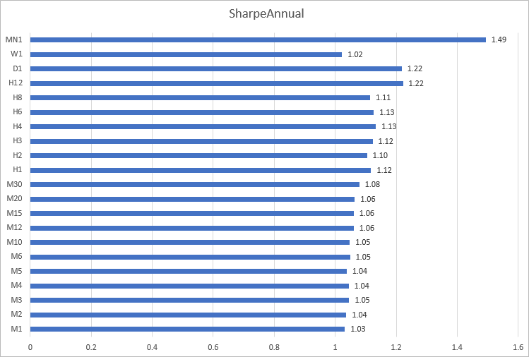
Let's construct a histogram of the Sharpe ratio on EURUSD for 2020 on the different timeframes. It can be seen here that calculations on minute timeframes, from M1 to M30, give close results: from 1.03 to 1.08. The most inconsistent results were obtained on timeframes from H12 to MN1.

Sharpe ratio calculation for GBPUSD, USDJPY and USDCHF for 2020

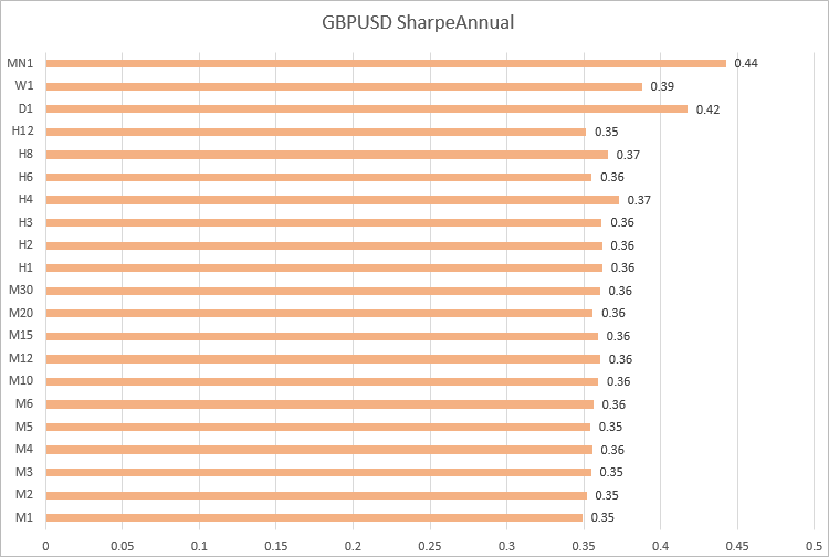
Let's perform similar calculations for three more currency pairs.

GBPUSD, Sharpe ratio values are similar on timeframes from M1 to H12.

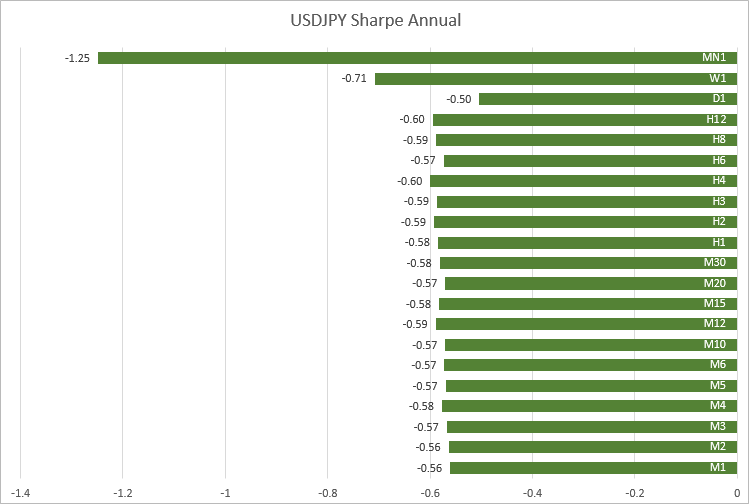
USDJPY, values are also close on timeframes from M1 to H12: -0.56 to -0.60.

USDCHF, similar values were obtained on timeframes from M1 to M30. As the timeframe increases, the Sharpe ratio fluctuates.

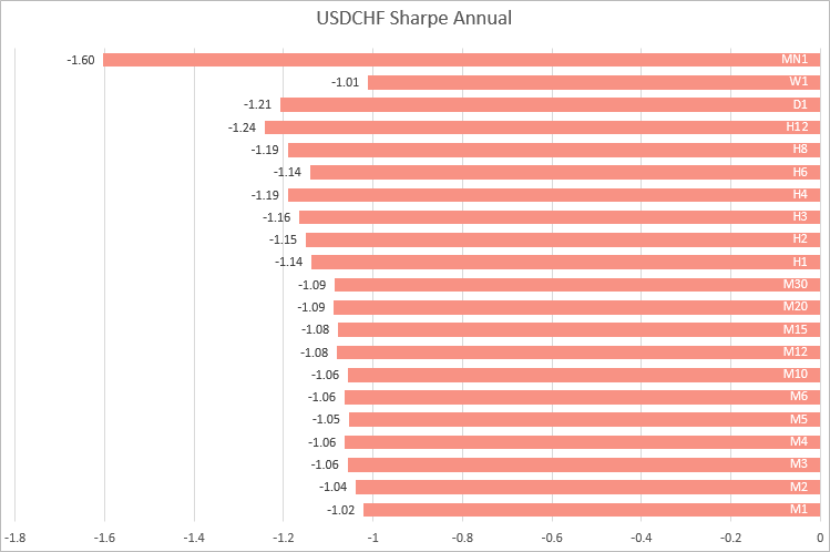
Thus, based on the examples of four major currency pairs, we can conclude that the most stable calculations of the Sharpe ratio are obtained on timeframes from M1 to M30. It means that it is better to calculate the ratio using lower-timeframe returns, when you want to compare strategies working on different symbols.

Calculating annual Sharpe ratio on EURUSD for 2020 by months

Let's use monthly returns of each month of 2020 and calculate the annual Sharpe Ratio on timeframes from M1 to H1. The full code of the CalculateSharpe_Months.mq5 script is attached to the article.

//--- structure to store returns
struct Return
  {
   double            ret;   // return
   datetime          time;  // date
   int               month; // month
  };
//+------------------------------------------------------------------+
//| Script program start function                                    |
//+------------------------------------------------------------------+
void OnStart()
  {
   SharpeMonths sharpe_by_months[];
//--- arrays of timeframes on which the Sharpe coefficient will be calculated
   ENUM_TIMEFRAMES timeframes[] = {PERIOD_M1,PERIOD_M2,PERIOD_M3,PERIOD_M4,PERIOD_M5,
                                   PERIOD_M6,PERIOD_M10,PERIOD_M12,PERIOD_M15,PERIOD_M20,
                                   PERIOD_M30,PERIOD_H1
                                  };
   ArrayResize(sharpe_by_months,ArraySize(timeframes));
//--- timeseries request parameters
   string symbol = Symbol();
   datetime from = D'01.01.2020';
   datetime to = D'01.01.2021';
   Print("Calculate Sharpe Annual on ",symbol, " for 2020 year");
   for(int i = 0; i < ArraySize(timeframes); i++)
     {
      //--- get the array of returns on the specified timeframe
      Return returns[];
      GetReturns(symbol,timeframes[i],from,to,returns);
      double avr,std,sharpe;
      //--- Calculate statistics for the year
      GetStats(returns,avr,std,sharpe);
      string tf_str = EnumToString(timeframes[i]);
      //--- calculate the annual Sharpe ratio for each month
      SharpeMonths sharpe_months_on_tf;
      sharpe_months_on_tf.SetTimeFrame(tf_str);
      //--- select returns for i-th month
      for(int m = 1; m <= 12; m++)
        {
         Return month_returns[];
         GetReturnsByMonth(returns,m,month_returns);
         //--- Calculate statistics for the year
         double sharpe_annual = CalculateSharpeAnnual(timeframes[i],month_returns);
         sharpe_months_on_tf.Sharpe(m,sharpe_annual);
        }
      //--- add Sharpe ratio for 12 months on timeframe i
      sharpe_by_months[i] = sharpe_months_on_tf;
     }
//--- display the table of annual Sharpe values by months on all timeframes
   ArrayPrint(sharpe_by_months,3);
  }

/*
Result

Calculate Sharpe Annual on EURUSD for 2020 year
             [TF]  [Jan]  [Feb] [Marc]  [Apr] [May] [June] [July] [Aug] [Sept]  [Oct] [Nov] [Dec]
[ 0] "PERIOD_M1"  -2.856 -1.340  0.120 -0.929 2.276  1.534  6.836 2.154 -2.697 -1.194 3.891 4.140
[ 1] "PERIOD_M2"  -2.919 -1.348  0.119 -0.931 2.265  1.528  6.854 2.136 -2.717 -1.213 3.845 4.125
[ 2] "PERIOD_M3"  -2.965 -1.340  0.118 -0.937 2.276  1.543  6.920 2.159 -2.745 -1.212 3.912 4.121
[ 3] "PERIOD_M4"  -2.980 -1.341  0.119 -0.937 2.330  1.548  6.830 2.103 -2.765 -1.219 3.937 4.110
[ 4] "PERIOD_M5"  -2.929 -1.312  0.120 -0.935 2.322  1.550  6.860 2.123 -2.729 -1.239 3.971 4.076
[ 5] "PERIOD_M6"  -2.945 -1.364  0.119 -0.945 2.273  1.573  6.953 2.144 -2.768 -1.239 3.979 4.082
[ 6] "PERIOD_M10" -3.033 -1.364  0.119 -0.934 2.361  1.584  6.789 2.063 -2.817 -1.249 4.087 4.065
[ 7] "PERIOD_M12" -2.952 -1.358  0.118 -0.956 2.317  1.609  6.996 2.070 -2.933 -1.271 4.115 4.014
[ 8] "PERIOD_M15" -3.053 -1.367  0.118 -0.945 2.377  1.581  7.132 2.078 -2.992 -1.274 4.029 4.047
[ 9] "PERIOD_M20" -2.998 -1.394  0.117 -0.920 2.394  1.532  6.884 2.065 -3.010 -1.326 4.074 4.040
[10] "PERIOD_M30" -3.008 -1.359  0.116 -0.957 2.379  1.585  7.346 2.084 -2.934 -1.323 4.139 4.034
[11] "PERIOD_H1"  -2.815 -1.373  0.116 -0.966 2.398  1.601  7.311 2.221 -3.136 -1.374 4.309 4.284

*/

It can be seen that the annual ratio values for each month are very close on all timeframes on which we performed calculations. For a better presentation, let's render the results as a 3D surface using an Excel diagram.

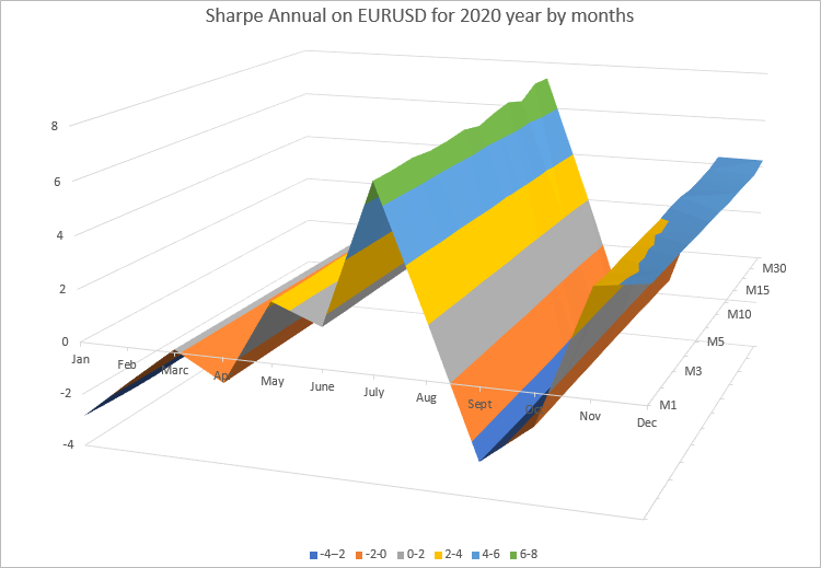
The diagram clearly shows that the values of the annual Sharpe ratio change every month. It depends on how EURUSD was changing this month. On the other hand, the annual Sharpe ratio for each month on all timeframes almost does not change.

Thus, the annual Sharpe Ratio can be calculated on any timeframe, while the resulting value also depends on the number of bars on which returns were obtained. It means that this calculation algorithm can be used in testing, optimization and monitoring in real time. The only prerequisite is to have a large enough array of returns.

Sortino ratio

In the Sharpe ratio calculation, the risk is the full volatility of quotes, both increase and decrease in the assets. But the increase in the portfolio value is good for the investor, while the loss is only connected with its decrease. Therefore, the actual risk in the ratio is overstated. The Sortino ratio developed in the early 1990s by Frank Sortino addresses this problem.

Like his predecessors, F. Sortino considers the future return as a random variable equal to its mathematical expectation, while the risk is considered as a variance. Return and risk are determined based on the historical quotes for a certain period. As in the Sharpe ratio calculation, return is divided by risk.

Sortino noted that the risk defined as the total variance of returns (or the full volatility) depends both on positive and negative changes. Sortino replaced the total overall volatility by semi-volatility which only considers a decrease in the assets. Semi-volatility is also referred to as harmful volatility, downside risk, downward deviation, negative volatility or the downside standard deviation.

The Sortino ratio calculation is similar to that of Sharpe, with the only difference being that positive returns are excluded from the volatility calculation. This reduces the risk measure and increases the ratio weight.

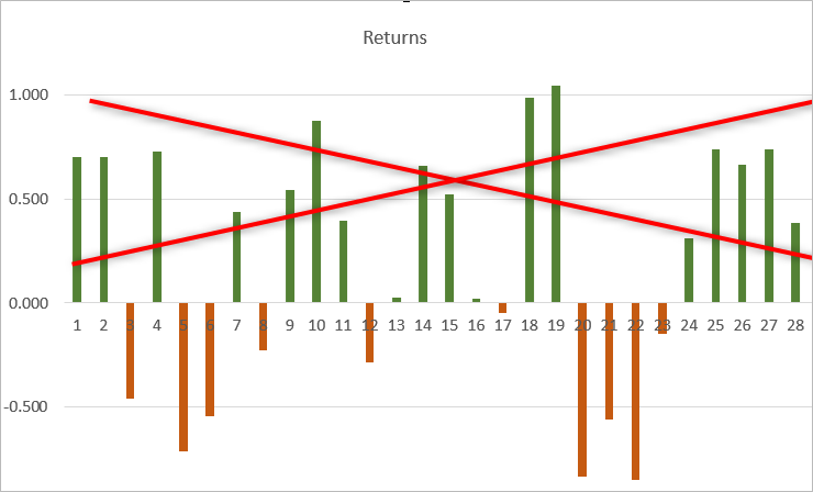
Code example calculating the Sortino ratio based on the Sharpe ratio. The semi-dispersion is calculated only using negative returns.

//+------------------------------------------------------------------+
//|  Calculates Sharpe and Sortino ratios                            |
//+------------------------------------------------------------------+
void GetStats(ENUM_TIMEFRAMES timeframe, const double & returns[], double & avr, double & std, double & sharpe, double & sortino)
  {
   avr = ArrayMean(returns);
   std = ArrayStd(returns);
   sharpe = (std == 0) ? 0 : avr / std;
//--- now, remove negative returns and calculate the Sortino ratio
   double negative_only[];
   int size = ArraySize(returns);
   ArrayResize(negative_only,size);
   ZeroMemory(negative_only);
//--- copy only negative returns
   for(int i = 0; i < size; i++)
      negative_only[i] = (returns[i] > 0) ? 0 : returns[i];
   double semistd = ArrayStd(negative_only);
   sortino = avr / semistd;   
   return;
  }

Script CalculateSortino_All_TF.mq5 attached to this article generates the following results on EURUSD, for 2020:

      [TF] [Minutes] [Rates]      [Avg]      [Std] [SharpeAnnual] [SortinoAnnual]    [Ratio]
[ 0] "M1"          1  373023 0.00000024 0.00014182     1.01769617      1.61605380 1.58795310
[ 1] "M2"          2  186573 0.00000048 0.00019956     1.02194170      1.62401856 1.58914991
[ 2] "M3"          3  124419 0.00000072 0.00024193     1.03126142      1.64332243 1.59350714
[ 3] "M4"          4   93302 0.00000096 0.00028000     1.02924195      1.62618200 1.57998030
[ 4] "M5"          5   74637 0.00000120 0.00031514     1.02303684      1.62286584 1.58632199
[ 5] "M6"          6   62248 0.00000143 0.00034122     1.03354379      1.63789024 1.58473231
[ 6] "M10"        10   37349 0.00000239 0.00044072     1.03266766      1.63461839 1.58290848
[ 7] "M12"        12   31124 0.00000286 0.00047632     1.04525580      1.65215986 1.58062730
[ 8] "M15"        15   24900 0.00000358 0.00053223     1.04515816      1.65256608 1.58116364
[ 9] "M20"        20   18675 0.00000477 0.00061229     1.04873529      1.66191269 1.58468272
[10] "M30"        30   12450 0.00000716 0.00074023     1.06348332      1.68543441 1.58482449
[11] "H1"         60    6225 0.00001445 0.00101979     1.10170316      1.75890688 1.59653431
[12] "H2"        120    3115 0.00002880 0.00145565     1.08797046      1.73062372 1.59068999
[13] "H3"        180    2076 0.00004305 0.00174762     1.10608991      1.77619289 1.60583048
[14] "H4"        240    1558 0.00005746 0.00200116     1.11659184      1.83085734 1.63968362
[15] "H6"        360    1038 0.00008643 0.00247188     1.11005321      1.79507001 1.61710267
[16] "H8"        480     779 0.00011508 0.00288226     1.09784908      1.74255746 1.58724682
[17] "H12"       720     519 0.00017188 0.00320405     1.20428761      2.11045830 1.75245371
[18] "D1"       1440     259 0.00035582 0.00470188     1.20132966      2.04624198 1.70331429
[19] "W1"      10080      51 0.00193306 0.01350157     1.03243721      1.80369984 1.74703102
[20] "MN1"     43200      12 0.00765726 0.01776075     1.49349076      5.00964481 3.35431926

It can be seen that in almost all timeframes Sortino value is 1.60 times the Sharpe ratio. Of course, there will not be such clear dependence when calculating the ratios based on trading results. Therefore, it makes sense to compare strategies/portfolios using both ratios.

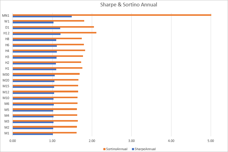
The difference between these two metrics is that the Sharpe ratio primarily reflects volatility, while the Sortino ratio really shows the ratio or return per unit of risk. But do not forget that the calculations are done based on history, so good results cannot guarantee future profits.

Example of Sharpe ratio calculation in the MetaTrader 5 Strategy Tester

Sharpe ratio was originally developed to evaluate portfolios containing stocks. Stock prices change every day, and therefore the value of assets also changes every day. By default, trading strategies do not imply the existence of open positions, so part of time the state of a trading account will remain unchanged. It means that when there are no open positions, we will receive zero return values, and thus Sharpe calculations will be wrong for them. Therefore, the calculations will only use the bars on which the trading account state has changed. The most suitable option is to analyze equity values on the last tick of each bar. This will allow the calculation of the Sharpe ratio with any tick generation mode in the MetaTrader 5 strategy tester.

Another point that should be taken into account is that the percentage price increment, which is usually calculated as Return[i]=(CloseCurrent-ClosePrevious)/ClosePrevious, has a certain disadvantage in calculations. It is as follows: if the price falls by 5% and then grows by 5%, we will not get the initial value. That is why, instead of the usual relative price increment, statistical studies usually utilize the price increment logarithm. Log returns (logarithmic returns) do not have this disadvantage of linear returns. The value is calculated as follows:

Log_Return =ln(Current/Previous) = ln(Current) — ln(Previous)

Log returns are convenient because they can be added together as the sum of logarithms is equivalent to the product of relative returns.

So, the Sharpe ratio calculation algorithm needs minimum adjustments.

//--- calculate the logarithms of increments using the equity array
   for(int i = 1; i < m_bars_counter; i++)
     {
      //--- only add if equity has changed
      if(m_equities[i] != prev_equity)
        {
         log_return = MathLog(m_equities[i] / prev_equity); // increment logarithm
         aver += log_return;            // average logarithm of increments
         AddReturn(log_return);         // fill the array of increment logarithms
         counter++;                     // counter of returns
        }
      prev_equity = m_equities[i];
     }
//--- if values are not enough for Sharpe calculation, return 0
   if(counter <= 1)
      return(0);
//--- average value of the increment logarithm
   aver /= counter;
//--- calculate standard deviation
   for(int i = 0; i < counter; i++)
      std += (m_returns[i] - aver) * (m_returns[i] - aver);
   std /= counter;
   std = MathSqrt(std);
//--- Sharpe ratio on the current timeframe
   double sharpe = aver / std;

The complete calculation code is implemented as an include file Sharpe.mqh which is attached to the article. To calculate the Sharpe ratio as a custom optimization criterion, connect this file to your Expert Advisor and add a few code lines. Let's see how to do it using the MACD Sample.mq5 EA from the standard MetaTrader 5 pack as an example.

#define MACD_MAGIC 1234502
//---
#include <Trade\Trade.mqh>
#include <Trade\SymbolInfo.mqh>
#include <Trade\PositionInfo.mqh>
#include <Trade\AccountInfo.mqh>
#include "Sharpe.mqh"
//---
input double InpLots          = 0.1;// Lots
input int    InpTakeProfit    = 50; // Take Profit (in pips)
input int    InpTrailingStop  = 30; // Trailing Stop Level (in pips)
input int    InpMACDOpenLevel = 3;  // MACD open level (in pips)
input int    InpMACDCloseLevel = 2; // MACD close level (in pips)
input int    InpMATrendPeriod = 26; // MA trend period
//---
int ExtTimeOut = 10; // time out in seconds between trade operations
CReturns   returns;
....
//+------------------------------------------------------------------+
//| Expert new tick handling function                                |
//+------------------------------------------------------------------+
void OnTick(void)
  {
   static datetime limit_time = 0; // last trade processing time + timeout
//--- add current equity to the array to calculate the Sharpe ratio
   MqlTick tick;
   SymbolInfoTick(_Symbol, tick);
   returns.OnTick(tick.time, AccountInfoDouble(ACCOUNT_EQUITY));
//--- don't process if timeout
   if(TimeCurrent() >= limit_time)
     {
      //--- check for data
      if(Bars(Symbol(), Period()) > 2 * InpMATrendPeriod)
        {
         //--- change limit time by timeout in seconds if processed
         if(ExtExpert.Processing())
            limit_time = TimeCurrent() + ExtTimeOut;
        }
     }
  }
//+------------------------------------------------------------------+
//| Tester function                                                  |
//+------------------------------------------------------------------+
double OnTester(void)
  {
//--- calculate Sharpe ratio
   double sharpe = returns.OnTester();
   return(sharpe);
  }
//+------------------------------------------------------------------+

Save the resulting code as "MACD Sample Sharpe.mq5" - the relevant file is also attached below.

Let's run a genetic optimization for EURUSD M10 2020, selecting a custom optimization criterion.

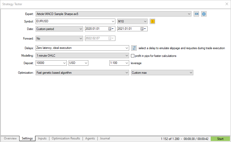
The obtained custom criterion values coincide with the Sharpe ratio calculated by the strategy tester. Now you know the calculation mechanisms as well as how to interpret the obtained results.

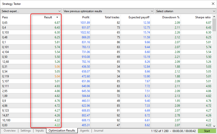
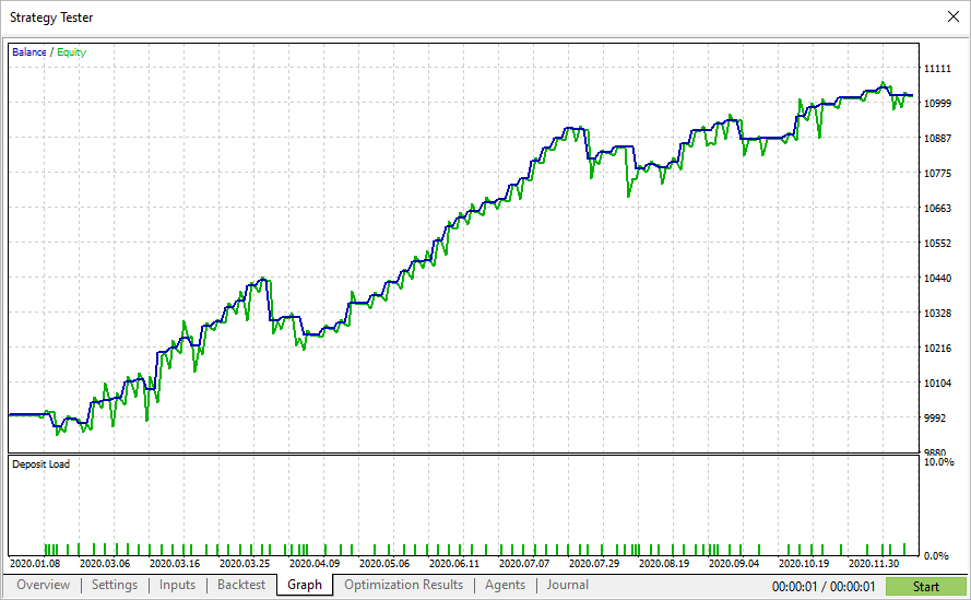
Passes with the highest Sharpe ratio do not always show the highest profit in the tester, but they allow finding parameters with a smooth equity graph. Such graphs usually don't show sharp growth, but there are also no big falls and equity drawdowns.

It means that using optimization by Sharpe ratio, it is possible to find more stable parameters, compared to other optimization criteria.

Advantages and disadvantages

Sharpe and Sortino ratios allow the determining of whether the received profit covers the associated risk or not. Another advantage over alternative risk measures is that the calculations can be applied to all types of assets. For example, you can compare gold to silver using the Sharpe ratio because it does not require a specific external benchmark to evaluate. Thus, the ratios can be applied to individual strategies or securities, as well as to asset or strategy portfolios.

The disadvantage of these tools is that the calculation assumes a normal distribution of returns. In reality, this requirement is rarely met. Nevertheless, Sharpe and Sortino ratios are the simplest and most understandable tools enabling the comparison of different strategies and portfolios.