Variational Mode Decomposition: Building the Solver, and Measuring What Hindsight Buys

Contents

• Introduction
• What this delivers
• The method: what VMD actually solves
• The frequency-domain plumbing
• The ADMM solver
• The causal boundary, and testing it by sabotage
• Reading a decomposition honestly
• Checking the solver against a reference
• What hindsight buys
• The indicator
• The strategy, and what it actually says
• Conclusion

Introduction

Price is a sum of things happening at different speeds: a multi-month trend, a multi-week swing, an intraday wobble, and noise that means nothing. Every trader draws that decomposition by eye on every change of timeframe. The question here is whether a machine can draw it, and what the drawing is worth once drawn.

The standard answers are unsatisfying. A moving average extracts a trend but lags it, throws the rest away, and needs you to pick the lookback. A Fourier transform assumes the frequencies never change, which is false for any market. Empirical Mode Decomposition is adaptive and popular, but it is a recipe rather than a stated problem and it suffers from mode mixing, one component quietly absorbing part of another.

Variational Mode Decomposition (Dragomiretskiy and Zosso, 2014) states a clear optimization: find K components that sum to the signal, each as narrow as possible around its own center frequency. It is solved by the alternating direction method of multipliers (ADMM) and yields clean bands with directly readable center frequencies. There is no VMD implementation on this site, so this article writes one.

The library is the first half; the second half decided how it had to be built. VMD is a batch algorithm: hand it a series and it optimizes over the whole thing at once, so a naive implementation decomposes the full chart history and plots the modes. The result looks convincing, fitting most historical turning points, and it is worthless, because every historical bar's mode value came from a window containing that bar's own future. This article measures how much of that picture is hindsight, on three real symbol/timeframe combinations against matched random walks.

You will end with a working library, an indicator whose every plotted point is computed once from a window ending at its own bar, a strategy whose stop, target and holding time come from the decomposition rather than from taste, and a set of numbers telling you what to believe.

What this delivers

The indicator draws three things on the main chart: the denoised signal, the trend mode alone, and a band showing how far this market currently wanders for no reason. A panel carries every mode's period in bars, its share of the energy, and a verdict on whether the window was solved well enough to read.

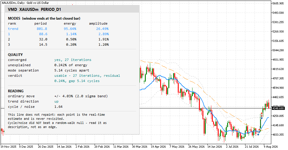
Fig. 1. The indicator on XAUUSD D1: every plotted point comes from a window ending at that bar, and the panel reports the modes and the solve quality

That is the visible product; the measured one matters more. Decomposing the whole visible history in one call, which almost every published VMD chart does, and comparing it bar by bar against the causal version gives this:

Symbol and timeframe	Median gap in trend value	Bars where the two point in opposite directions
XAUUSD D1	1318 bp	31.0%
XAUUSD H1	40 bp	33.9%
EURUSD H1	15 bp	24.2%

A batch chart is not a smoother version of the causal one. On roughly one bar in three, across the three combinations tested, it points the other way. That table is why the indicator in Fig. 1 is built the way it is.

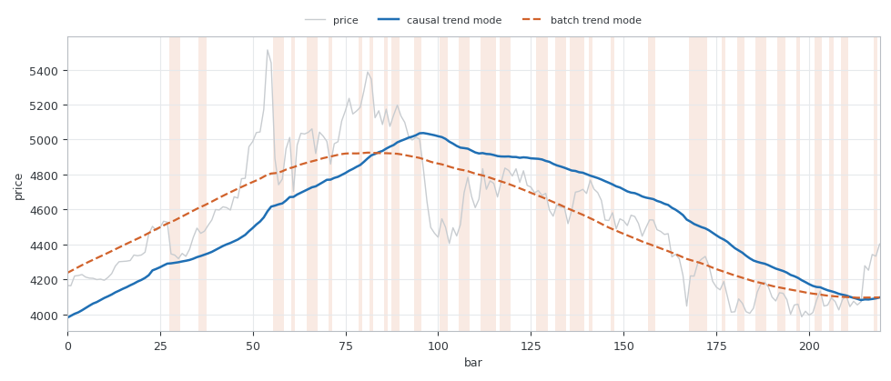
Fig. 2. The same trend mode computed two ways over the same bars, with the disagreement in direction shaded

The method: what VMD actually solves

VMD asks for K modes u_k that add up to the input f, each concentrated around its own center frequency w_k. "Concentrated" is made precise by taking each mode's analytic signal, shifting it to baseband, and penalizing the squared norm of its time derivative. A narrow band changes slowly once shifted down, so a small penalty means a tight mode.

Written out, the constrained problem is:

minimize over {u_k},{w_k}: sum_k || d/dt [ analytic(u_k)(t) * exp(-j*w_k*t) ] ||^2 subject to sum_k u_k = f

The constraint is handled with an augmented Lagrangian, which adds a quadratic penalty and a dual variable lambda, and is solved by alternating: hold everything else fixed and update one block at a time. In the frequency domain each update has a closed form, which makes VMD cheap despite looking heavy.

Updating mode k is a Wiener filter on whatever the other modes have not explained:

u_k(w) = ( f(w) - sum_{i != k} u_i(w) - lambda(w)/2 ) / ( 1 + alpha*(w - w_k)^2 )

The denominator is the whole idea. At w = w_k it equals 1 and the residual passes through untouched; far from w_k it grows as alpha times the squared distance and crushes whatever is there. So alpha sets how wide each band may be.

The center frequency is the power-weighted centroid of the mode just built:

w_k = sum_w w*|u_k(w)|^2 / sum_w |u_k(w)|^2

The dual variable takes an ascent step on how badly the modes fail to add up:

lambda(w) = lambda(w) + tau*( sum_k u_k(w) - f(w) )

Three parameters fall out. K is how many modes you want. alpha is the bandwidth penalty, so a large alpha gives narrow, well-separated bands. tau is the dual ascent step, and setting it to zero relaxes the sum-to-signal constraint, the right choice when the input is noisy.

Fig. 3 shows this on a signal where the answer is known: three cosines at 4, 16 and 48 cycles across the window, summed, then handed to the solver with no hint about what went in.

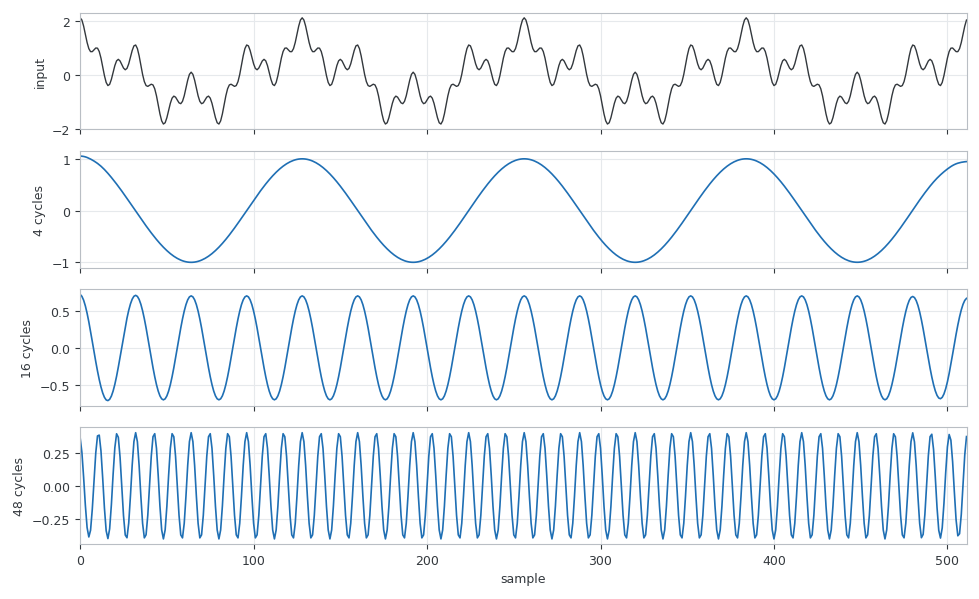
Fig. 3. A sum of three tones and the three modes the solver pulls back out of it, with the recovered cycle counts

The library recovers 4.000, 15.999 and 48.001 cycles, the sanity check every decomposition should pass before it is pointed at price.

The frequency-domain plumbing

Every update above is a pointwise operation on a spectrum; nothing in the iteration transforms anything. The input is transformed once before the loop and the K finished modes once after it, so a decomposition costs K+1 transforms however many iterations it runs. The iteration count, not the transform, sets the price.

The transform is an iterative radix-2 Cooley-Tukey in VMDTransform.mqh. Two details in it are easy to get wrong.

First, twiddle factors are evaluated with cosine and sine per butterfly rather than carried as a running product. The running product is faster but accumulates drift, and that drift feeds back into the solver: the filter divides by 1 + alpha*(w - w_k)^2 and w_k is a power-weighted centroid of the same spectrum.

Second, the shift that moves the zero frequency to the middle of the array is its own inverse at even length, being nothing but a swap of the two halves, which is why the library has one routine rather than a forward and inverse pair:

//+------------------------------------------------------------------+
//| Move the zero frequency to the middle of the array               |
//|                                                                  |
//|  For an EVEN length this is just a swap of the two halves, and   |
//|  that operation is its own inverse - which is why forward and    |
//|  inverse shifts are one routine here rather than two. Odd        |
//|  lengths would need the usual off-by-one pair, and are refused:  |
//|  the solver only ever shifts arrays of length T = 2N.            |
//|                                                                  |
//|  After the shift, index T/2 carries the zero frequency, indices  |
//|  below it the negative frequencies and indices above it the      |
//|  positive ones. The solver relies on exactly that layout when it |
//|  zeroes the negative half to build the analytic signal.          |
//+------------------------------------------------------------------+
bool CVMDTransform::Shift(double &a[])
  {
   int n = ArraySize(a);
   if(n < 2 || (n % 2) != 0)
    {
     PrintFormat("VMDTransform::Shift - length %d is not even", n);
     return false;
    }
   int h = n >> 1;
   for(int i = 0; i < h; i++)
    {
     double t = a[i];
     a[i]     = a[i + h];
     a[i + h] = t;
    }
   return true;
  }

Before the transform runs, the window is mirrored. With h = N/2, the first h bars are reflected onto the front and the last h onto the back, so a window of N bars is actually solved at length T = 2N. Without it the first and last bars look like a discontinuity to a periodic transform, and every mode picks up a spurious jump there. With it the extended array is continuous across the original window's ends, though not smooth: reflection reverses the slope at each join, so the mirror removes the step and leaves a kink. The step is the part the spectrum reacts to most.

That has a consequence that comes back in the results. The ends of the window are the least trustworthy part of any decomposition, since half their supporting data is reflection rather than observation, and in trading the end of the window is the only part you can act on.

//--- reflect the first half at the front and the last half at the back
   for(int i = 0; i < h; i++)
     m_mirror[i] = f[h - 1 - i];
   for(int i = 0; i < N; i++)
     m_mirror[h + i] = f[i];
   for(int i = 0; i < h; i++)
     m_mirror[h + N + i] = f[N - 1 - i];

   for(int i = 0; i < T; i++)
    {
     m_fRe[i] = m_mirror[i];
     m_fIm[i] = 0.0;
    }
   if(!CVMDTransform::FFT(m_fRe, m_fIm, false))
     return false;
   if(!CVMDTransform::Shift(m_fRe) || !CVMDTransform::Shift(m_fIm))
     return false;

After the shift, the negative half of the spectrum is zeroed. That converts the real signal to its analytic counterpart, which is what the derivation assumes, and it means every mode the solver produces is one-sided too. The Hermitian symmetry is put back by hand at the end, before the inverse transform. The construction is a little more than a dropped half-array: the Nyquist bin lands at index 0 and is zeroed with the negative frequencies, the surviving bins keep their original amplitudes rather than being doubled, and the zero-frequency bin survives carrying almost nothing because the mean was already removed.

Because the transform is radix-2 and the solve happens at T = 2N, N must be a power of two. There is no zero-padding escape here of the kind a convolution enjoys. That is not because padding changes the spectrum while mirroring does not, since both change it, but because they change it differently: zeros append a flat segment unrelated to the series, while the reflection appends samples with the same local level and variance. No measurement here puts a number on that gap. The data layer therefore snaps a requested window down to the nearest power of two.

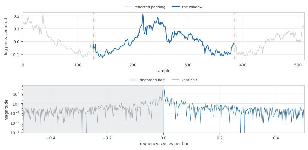
Fig. 4. The window is reflected to twice its length before transforming, and the negative half of the centered spectrum is discarded

The ADMM solver

The solver lives in VMDCore.mqh. Its inner sweep is the three updates from Section 3 over K modes; the excerpt below is the mode update: the accumulator, the Wiener filter, the centroid.

      for(int k = 0; k < K; k++)
       {
        int cur  = (C * K + k) * T;
        int prvK = (P * K + k) * T;

        //--- the accumulator holds "every mode except this one", mixing the
        //--- already-updated modes of this sweep with last sweep's rest
        if(k == 0)
         {
          int prvLast = (P * K + (K - 1)) * T;
          for(int i = 0; i < T; i++)
           {
            m_sumRe[i] += m_upRe[prvLast + i] - m_upRe[prvK + i];
            m_sumIm[i] += m_upIm[prvLast + i] - m_upIm[prvK + i];
           }
         }
        else
         {
          int curPrev = (C * K + (k - 1)) * T;
          for(int i = 0; i < T; i++)
           {
            m_sumRe[i] += m_upRe[curPrev + i] - m_upRe[prvK + i];
            m_sumIm[i] += m_upIm[curPrev + i] - m_upIm[prvK + i];
           }
         }

        //--- Wiener filter of the residual around this mode's frequency
        double wk = m_om[P * K + k];
        for(int i = 0; i < T; i++)
         {
          double d   = m_freqs[i] - wk;
          double den = 1.0 + m_alpha * d * d;
          m_upRe[cur + i] = (m_fRe[i] - m_sumRe[i] - 0.5 * m_lmRe[P * T + i]) / den;
          m_upIm[cur + i] = (m_fIm[i] - m_sumIm[i] - 0.5 * m_lmIm[P * T + i]) / den;
         }

        //--- power-weighted centroid over the positive half
        if(m_DC && k == 0)
          m_om[C * K + k] = 0.0;
        else
         {
          double num = 0.0, den2 = 0.0;
          for(int i = half; i < T; i++)
           {
            double pw = m_upRe[cur + i] * m_upRe[cur + i]
                     + m_upIm[cur + i] * m_upIm[cur + i];
            num  += m_freqs[i] * pw;
            den2 += pw;
           }
          m_om[C * K + k] = (den2 > 0.0 ? num / den2 : 0.0);
         }
       }

The accumulator deserves a note. Updating mode k naively needs the sum of all the other modes, a fresh O(K*T) sum for every mode on every sweep. Instead m_sumRe is carried across the run and corrected by two terms: add the mode that just moved out of the "others" set, subtract the one moving in. That mixes the already-updated modes of this sweep with the previous sweep's rest, which is the Gauss-Seidel ordering the method expects. Whether the running sum is right is not visible here: it also depends on the initial fill before the first sweep and on the row swap that makes P the previous sweep and C the current one, both outside this loop. The tests check the consequence, planted tones at the right frequencies, not the recurrence alone.

The indices P and C are the second thing worth pointing at. The reference stores all iterations in an array of size maxIter x 2N x K, about 32 MB per call at N = 512 and K = 4. The recurrence never reads further back than one sweep, so this solver keeps two rolling rows and swaps them: the same arithmetic in roughly 130 KB, which matters because a rolling indicator calls it once per bar.

One inherited quirk is reproduced deliberately. The reference reads its answer from the second to last ADMM row rather than the last one, a detail carried down from the original MATLAB. It is what every published VMD result was produced with, so the solver matches it, and removing it shifts the output by a small amount that looks exactly like a tolerance problem in a cross-check and is not one. That is a compatibility decision and only that: matching the reference says nothing about which row is the better answer, since near convergence the two differ by less than the tolerance.

Convergence is not guaranteed, and one series will not show you how often it fails. Over 40 walks at N = 512, K = 4, alpha = 2000 and tol = 1e-6, 35 converged out of 40, with the iteration count spanning 71 to 499 and a median of 218. So roughly one window in eight runs out of iterations, which makes the converged flag a live quality gate, not a formality.

Both K and alpha buy convergence, and alpha is the sharper.

Setting	Converged, out of 40 walks	Median iterations
K = 2	40	98
K = 4	35	218
K = 8	27	337
alpha = 500	23	441
alpha = 2000	35	218
alpha = 5000	35	141

A small alpha means wide bands that overlap and fight, the least stable setting available. A large K costs twice over, for the extra modes and the extra sweeps they need.

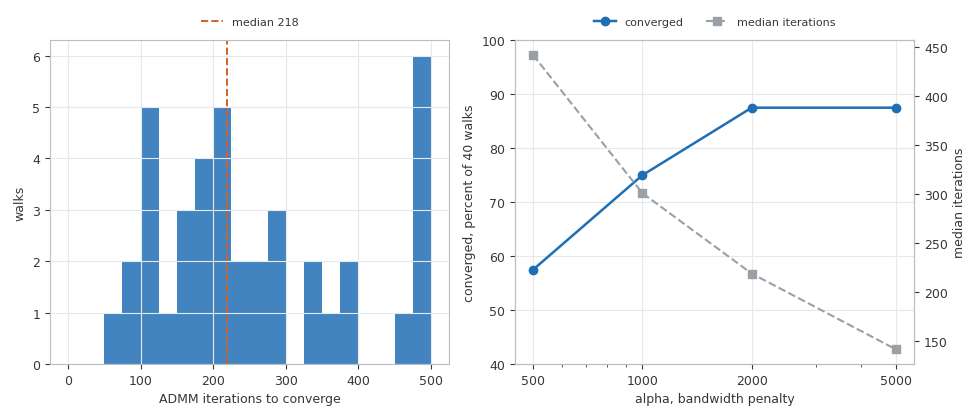
Fig. 5. Iteration counts over 40 matched random walks, and how the converged fraction moves with the bandwidth penalty

The cost that follows from all this is set by the iteration count. Each sweep is linear in N at fixed K while the K+1 transforms outside the loop are N log N, so the sweeps dominate at these window sizes; at much larger N the transforms would begin to show. In MetaTrader 5, as the minimum over five repetitions, one ADMM iteration costs about 44, 79 and 144 microseconds at N = 256, 512 and 1024 with K = 4; three runs of the same test reported those numbers as high as 61, 98 and 261. The minimum is a lower bound on the solver's cost, not the latency to expect, and the test reports no median or tail, so plan against the upper figures. The spread is most likely contention with other terminal activity, but that is a reading rather than a measurement: no profiling or isolated replay was run. At the shipped tolerance a price window runs about 150 to 270 iterations, so one decomposition lands near 12 to 26 milliseconds at N = 512. Loosening the tolerance from 1e-9 to 1e-4 saves about 40% of that and moves the answer by 0.095% of range, which is why 1e-4 is the default.

Important: GetTickCount cannot time this: its resolution on Windows is about 15 ms, the same order as a whole decomposition, and it reported 0, 15 and 15 ms for three runs that differed by a factor of four. Use GetMicrosecondCount and print the observed range.

The causal boundary, and testing it by sabotage

Everything so far decomposes an array. Which array it is allowed to see is the decision that makes the library usable, and it lives in one class rather than in the indicator and the strategy.

CVMDData takes a bar anchor and produces the window ending at that bar, transformed three ways. Prices are log-transformed, because a 1% move should count the same at 2000 as at 3000 and because mode amplitudes then read directly as fractional moves, which is where the strategy's target comes from. Then the mean is removed, then the length is snapped to a power of two.

//+------------------------------------------------------------------+
//| One window from the chart, anchored at a bar SHIFT               |
//|                                                                  |
//|  endShift is a shift, so 1 is the last CLOSED bar and 0 is the   |
//|  bar still forming. Callers that pass 0 are decomposing a bar    |
//|  that is still changing, and every reading taken from it will    |
//|  change with it; the library allows it but the indicator and the |
//|  EA both anchor at 1 on purpose.                                 |
//+------------------------------------------------------------------+
bool CVMDData::BuildFromChart(const string symbol, const ENUM_TIMEFRAMES tf,
                              const int endShift, double &out[])
  {
   int N = m_window;
   if(endShift < 0)
    {
     Print("VMDData - endShift cannot be negative");
     return false;
    }

   double closes[];
   ArraySetAsSeries(closes, true);
   int got = CopyClose(symbol, tf, endShift, N, closes);
   if(got != N)
    {
     PrintFormat("VMDData - asked for %d bars at shift %d, got %d", N, endShift, got);
     return false;
    }

   ArrayResize(out, N);
   double sum = 0.0;
   for(int i = 0; i < N; i++)
    {
     //--- closes[] is newest-first; the solver wants oldest-first
     double v = closes[N - 1 - i];
     if(m_useLog)
      {
       if(v <= 0.0)
        {
         Print("VMDData - non-positive price cannot be log transformed");
         return false;
        }
       v = MathLog(v);
      }
     out[i] = v;
     sum   += v;
    }

   m_mean = sum / N;
   for(int i = 0; i < N; i++)
     out[i] -= m_mean;

Removing the mean is free mathematically, since subtracting a constant moves only the zero-frequency term, and arithmetically it is the difference between a working library and a broken one: the mean of log gold is an enormous spike at the exact center of the spectrum, it survives the analytic-signal step, and every mode's Wiener filter then fights over it. The removed mean is kept so a caller can map a mode value back to price.

Now the part that matters. Claiming a library is causal is easy. VMD_Test_Facade.mq5 checks it by sabotage: decompose at a bar, overwrite every later bar with arbitrary values, decompose again, and demand the two answers be identical.

//--- now destroy everything strictly after the anchor
   double poisoned[];
   ArrayCopy(poisoned, prices);
   for(int i = anchor + 1; i < n; i++)
     poisoned[i] = 1.0 + 1000.0 * MathAbs(NextR());

   CVMD b;
   b.SetWindow(256);
   b.SetK(4);
   b.SetTol(1e-6);
   Check(b.DecomposeSeries(poisoned, anchor), "decomposed the poisoned series");

   double worstMode = 0.0, worstOm = 0.0;
   for(int k = 0; k < K; k++)
    {
     worstOm = MathMax(worstOm, MathAbs(omA[k] - b.Omega(k)));
     for(int i = 0; i < N; i++)
       worstMode = MathMax(worstMode,
                              MathAbs(modesA[k * N + i] - b.ModeValue(k, i)));
    }
   Check(worstMode == 0.0 && worstOm == 0.0,
       "the future changed nothing: bit-identical",
       StringFormat("mode diff %.3e, omega diff %.3e", worstMode, worstOm));

The measured difference is 0.000e+00 on both the modes and the frequencies. The test then does the opposite check, moving the anchor bar itself by 5% and demanding the answer does change, because a function that ignores its input would also pass the first half. Two limits on what that proves. Comparing against zero exactly is right inside one process on one build, where both calls take identical arithmetic paths, but it is not a benchmark that would survive a change of compiler. And it exercises the array path; the chart path is covered by the indicator verification in Section 10.

Reading a decomposition honestly

A decomposition always returns something: modes for a pure trend, for noise, and for a window where the solver quit without settling, and on a chart all three look equally convincing. So the numbers that say whether the answer means anything travel with it in the same struct.

   int               K;                 // number of modes
   int               n;                 // samples per mode
   double           modes[];            // K*n, mode k at [k*n .. k*n+n-1]
   double           omega[];            // K center frequencies, cycles per bar
   double           energy[];           // K mode energies as a fraction of input

   int               iters;             // ADMM iterations actually run
   int               maxIters;          // the cap it was allowed
   bool              converged;         // stopped by tolerance, not by the cap
   double           uDiff;              // the convergence measure at the end

   double           residFrac;          // unexplained energy / input energy
   double           residMaxAbs;        // largest single-sample residual
   double           minGapCycles;       // smallest adjacent omega gap, in cycles
   bool              omegaSorted;       // did the solver return them in order

   bool              valid;             // the inputs were accepted at all

Three of these need explaining.

residFrac is not an epsilon check. The obvious property to assert is that the modes sum back to the input, which is the constraint the problem states, and the solver meets it exactly at no tau: at tau = 0 the constraint is deliberately relaxed, and with tau non-zero the dual ascent drives the sum toward the input without arriving, because the Wiener filters have finite bandwidth and some energy never lands in any mode. A three-tone signal leaves 8.7e-03 even at tau = 1.0, and a random walk leaves about 3% of range. Over 40 walks at K = 4 the unexplained fraction is 5.8e-03 at the median and 1.2e-02 at the ninetieth percentile, and the shipped threshold sits above that percentile: an empirical setting from forty walks at one window length, not a derived bound, with its stability across windows and instruments untested.

minGapCycles is the K selection signal. Ask for more modes than the signal supports and two collapse onto the same frequency, at which point the pair is one mode reported twice. On one walk the smallest gap between adjacent center frequencies held between 3.5 and 4.8 cycles from K = 2 through K = 6 and then fell to 1.43 at K = 7, while the residual stopped improving. That collapse is the signal that K is too large, and it is reported per window rather than baked into a rule, because the collapse point is series dependent: other walks hold their separation to K = 8 and never collapse at all. So there is no K that is right in general and no rejection rule here either; what is reproducible is the procedure, which is to sweep K on your own series and stop before the smallest gap collapses while the residual stops improving.

Mode order is not guaranteed. With uniform frequency initialization the planted tones at 4, 16 and 48 cycles came back in the order 4, 48, 16, and on one walk it invented a 156-cycle mode where zero initialization gave a sensible spread. The facade therefore rebuilds a frequency ranking after every decomposition and every accessor works in rank, so rank 0 is the slowest component whatever index the solver gave.

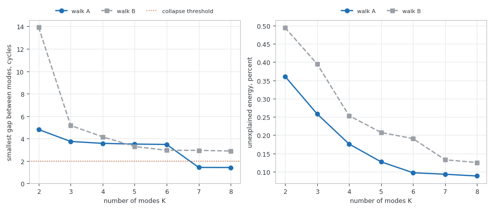
Fig. 6. The smallest gap between adjacent modes against K, on two random walks: one collapses past the usable level at K = 7, the other holds its separation throughout

On top of these the facade exposes four readings a strategy may use, each derived from the decomposition rather than chosen: a mode's swing amplitude (its root mean square times the square root of two, exact for a sinusoid), its half period in bars, the noise width, the standard deviation of everything the denoised signal dropped, and a regime ratio.

That last one needs stating, because the obvious regime measure fails on price: log price is dominated by its trend, so rank 0 carried 95.7% of the energy on XAUUSD D1, the slow-energy reading came out at 0.9932, and a gate at 0.90 would pass every window ever presented to it. Dropping rank 0 and asking about the rest gives a number with room to move:

//+------------------------------------------------------------------+
//| Oscillatory structure against oscillatory churn, trend EXCLUDED  |
//|                                                                  |
//|  SlowEnergy is the obvious regime reading and on price data it   |
//|  is nearly useless, which only a real chart showed: log price is |
//|  dominated by its trend, so rank 0 carried 95.7% of the energy   |
//|  on XAUUSD D1 and SlowEnergy(2) read 0.9932. A gate at 0.90      |
//|  would pass every window ever presented to it.                   |
//|                                                                  |
//|  This ratio drops rank 0 entirely and asks the question that is  |
//|  actually open: of the part of the move that is NOT the trend,   |
//|  how much sits in slow swings rather than in fast churn. On the  |
//|  same XAUUSD window that is 1.07% against 0.46% + 0.20%, a ratio |
//|  of about 1.6 - a number with room to move in both directions.   |
//|                                                                  |
//|  Returns 0 when there is no oscillatory energy at all, and a     |
//|  large finite number rather than infinity when there is no       |
//|  churn, so a caller can compare it without special cases.        |
//+------------------------------------------------------------------+
double CVMD::CycleToNoise(const int cycleRanks) const
  {
   if(!m_res.valid || m_res.K < 3)
     return 0.0;
   int hi = MathMin(MathMax(cycleRanks, 1), m_res.K - 2);

   double cyc = 0.0, noise = 0.0;
   for(int r = 1; r <= hi; r++)
     cyc += EnergyOfRank(r);
   for(int r = hi + 1; r < m_res.K; r++)
     noise += EnergyOfRank(r);

   if(cyc <= 0.0)
     return 0.0;
   if(noise <= 0.0)
     return 1e6;
   return cyc / noise;
  }

Whether that is worth gating on is what the next two sections answer.

Checking the solver against a reference

A from-scratch numerical solver is worth as much as its verification. VMD is lucky here: the widely used Python reference (vmdpy) is fully deterministic, its center frequencies starting either at zero or at a fixed uniform spread with no random seeding, which turns the cross-check from a statistical comparison into an equality.

The verification uses two Python implementations. The first is the reference itself. The second is restructured the way the MQL5 code had to be written: two rolling ADMM rows instead of a full history, a hand-written radix-2 transform instead of a library call, real arrays instead of complex ones. Checking against both separates two failures. Agreeing with the reference but not the restructured version means the port drifted; the reverse means the blueprint was wrong to begin with.

An MQL5 script exports eleven configurations, dumping the window the solver saw along with its modes, frequencies and diagnostics. Doubles are written with %.17g, which round-trips an IEEE 754 double exactly, so the comparison is made at the level of the arithmetic rather than at six decimals; that assumes a period decimal separator, and on a comma-decimal environment the Python side splits the row on the wrong character and fails outright rather than quietly shifting a digit. The cases exercise every branch: both initializations, the zero-frequency constraint on and off, tau zero and non-zero, three window sizes, four values of K, and two windows of real gold bars.

Comparison	Worst disagreement
Modes, relative to input scale	1.29e-13
Center frequencies, absolute	4.11e-14
Unexplained energy fraction	1.6e-15 relative
ADMM iteration count	exact on all 11 cases

The iteration count matching exactly on every case is the strongest line in that table. The two implementations did not merely arrive at the same answer, they took the same number of steps to get there, which requires the convergence measure to track closely enough at every sweep to cross the tolerance on the same one. That is not agreement at the last digit: two runs that differ slightly can still cross a threshold together.

Alongside the reference comparison the suite checks things that need no reference: the transform against a direct O(N^2) discrete transform, against closed forms for a constant, an impulse and a pure cosine, and against Parseval's identity and linearity. Those catch what an equality check cannot, both implementations being wrong in the same way.

What hindsight buys

Here is the experiment the library was built for.

Roll a causal decomposition forward one bar at a time and record, for each anchor, the trend value assigned to the bar at the window's edge and to the bars behind it. A bar gets one value as the newest bar in the window, and a different one once it is one, five or twenty-five bars old. The gap between them is repaint.

The comparison needs a null, so here is the null. Each matched walk is built in log space from the real series' own per-bar log-return standard deviation, with no drift term, from a fixed-seed linear congruential stream whose draws are six uniforms summed to unit variance. It carries gold's volatility but neither its trend nor its tails, and the same seed reproduces every number here. The repaint table uses one such walk and the regime band five. The forty behind the convergence table in Section 5, which are also the forty behind the residual percentiles in Section 7, are a simpler null: plain unit-variance Gaussian walks from the Python phase, matched to no instrument, because neither convergence nor the residual floor is a property of a symbol.

Here is the drift on XAUUSD D1 over 250 rolling windows, in basis points of price:

Bar age	Median drift, real	Median drift, matched random walk	Direction reversed, real	Direction reversed, null
1 bar	17.5 bp	14.7 bp	13.7%	13.3%
5 bars	81.3 bp	68.4 bp	25.3%	23.3%
25 bars	191.9 bp	175.8 bp	31.6%	37.8%

The two drift columns sit at the same scale, and at 25 bars the null reverses direction more often than the real series does. That comparison is the finding: on these series, most of the repaint comes from the method rather than from the market. A random walk matched to gold's own per-bar volatility, carrying no deterministic cycles, repaints by a comparable amount. What one matched walk cannot do is separate the two sources, and the gap that remains is not zero: real drift sits above its null at all three ages, by 8 to 16 percent of the drift itself. A comparable scale is not a measurement of independence, so a drift reading is mostly method with a remainder that one walk cannot size.

The pattern holds on the other two combinations. On XAUUSD H1 the one-bar drift is 3.6 bp against a null of 4.0, and on EURUSD H1 it is 0.8 bp against 1.1; in both the null repaints slightly more than the real series.

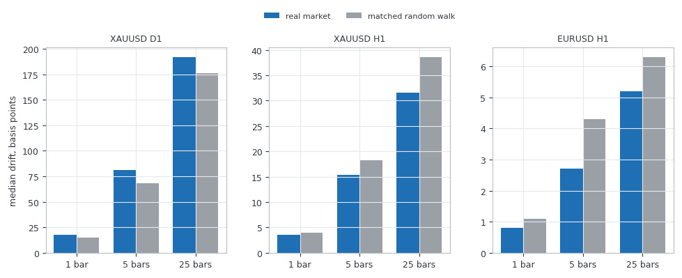
Fig. 7. Trend-value drift as a bar ages, real data against a volatility-matched random walk, on three symbol and timeframe combinations

The endpoint profile answers a related question badly. Drift from the freshest reading grows roughly linearly with distance from the window edge, out to the 50 bars measured, with no sign of stabilization: on XAUUSD D1 it runs 17, 35, 54, 64, 81 basis points at one through five bars back and keeps climbing. There is no lag at which the reading settles.

The practical response is to compute each point once, from the window ending at its own bar, and never recompute it. That plot does not repaint, not because repaint was engineered away, but because the real-time estimate is what gets drawn and is then left alone. Two senses of the word are worth keeping apart: causal means the value uses no bar after its own, which the data layer enforces and the sabotage test checks, but it is not stable, since the value sits at the window edge where half its support is reflection. Drawing it once fixes the picture, not the uncertainty.

The regime reading did not survive its own null. Comparing the real median of the cycle-to-noise ratio from Section 7 against the band produced by five matched walks on the same settings:

Symbol and timeframe	Real median	Null band over 5 walks	Verdict
XAUUSD D1	2.264	inside	does not separate
XAUUSD H1	2.069	2.412 to 4.706	below the null
EURUSD H1	2.823	2.658 to 3.958	does not separate

In no market did real data look more cyclical than noise, and on gold H1 it looked less so. A gate on that ratio would filter nothing while implying a discrimination that does not exist, so it ships turned off.

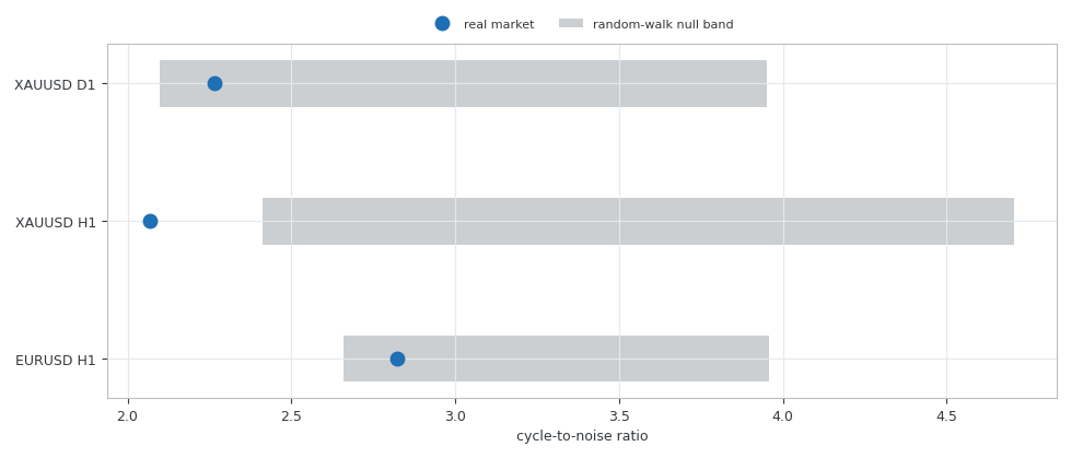
Fig. 8. The regime ratio against the band spanned by five matched random walks, on each symbol and timeframe

The scope of this should be read off the design. Three symbol and timeframe combinations, 250 rolling anchors each, one matched walk behind the repaint table and five behind the regime band: every number above is a point estimate with no confidence interval, no p-value and no bootstrap behind it, and the percentages are quoted more precisely than the sample supports. That is enough to show that batch and causal readings differ by a lot, and that a series with no cycles drifts by a similar amount. It is not enough to put a figure on either difference, or to say whether the pattern survives on instruments not looked at.

None of this makes the decomposition useless. It makes it descriptive. The modes are a well-defined and reproducible summary of what a window contains, and the noise width is a genuine volatility estimate. What the measurements refuse is the leap from "this is a clean decomposition" to "this tells me something the market did not already say."

The indicator

VMD_Decomposition.mq5 plots four buffers on the main chart: the denoised signal, the trend mode, and a band at plus and minus a chosen number of noise standard deviations around the denoised line, all mapped back through the log and the removed mean so they sit in price units. One caution about reading them: the modes add in log space, not in price, so exponentiating one mode does not give a price component that the others add to. The trend line is that mode's level expressed as a price, not a split of price into additive parts.

The important part is the calculation policy. On the first pass it wipes every buffer and computes each displayed bar once from its own causal window; on every later call it computes only newly closed bars. A value already written is never recomputed.

   //--- newest CLOSED bar. The forming bar is never decomposed: its close
   //--- is still moving, so any reading taken from it moves with it.
   int lastClosed = rates_total - 2;
   int first     = MathMax(lastClosed - InpHistoryBars + 1, need);

The history cap is a cost decision, not a convention. One decomposition costs a few milliseconds and a first load pays that once per displayed bar. Measured on this build the default of 150 bars took 1017 ms on XAUUSD D1 (6.8 ms per bar) and 222 ms on EURUSD H1 (1.5 ms per bar), each the fastest of several loads; the slowest of the same loads were 1244 ms and 352 ms, which are the figures to plan against. A 500-bar setting would be three times worse for no extra information, since the older bars carry the reading they would have carried anyway.

The panel is drawn with chart objects, a background rectangle plus text labels, rather than Comment. That is the only way to get aligned columns and a readable box, but chart objects do not clip their text: a value too long for the panel renders out over the chart, and no buffer assertion can see that because buffers know nothing about labels. Any long value is therefore wrapped at a character count derived from the panel width and font size, and the panel reports the widest label it drew so an overflow announces itself in the log. That is a log-level guard and not a visual assertion: nothing inspects the rendered panel, so the last check on its geometry is the eye.

Because an indicator cannot assert on itself, VMD_Verify_Indicator.mq5 drives it through iCustom and checks the buffers from outside: that exactly the display window is filled and older bars left empty, that the band brackets the denoised line, that the values sit in price range rather than log units, that the denoised line is smoother than price, and that the forming bar mirrors the last closed one instead of leading it.

Its last check is the one that matters. The script decomposes the same bar itself and compares its answer against what the indicator plotted there; if those agree, the plotted point came from a window ending at its own bar. On XAUUSD D1 and EURUSD H1 the worst disagreement across five probe bars was 0.000e+00. That is five probe bars on two charts at the shipped settings: strong evidence about the path the indicator takes, silent about very small windows, too little history, or a symbol change mid-session.

The strategy, and what it actually says

VMD_Cycle_EA.mq5 trades the oscillatory mode: long when rank 1 crosses up through zero while the trend mode is rising, short on the mirror image. That entry is ordinary; what makes it a VMD strategy is the risk, since every number comes out of the decomposition:

   //--- log-unit distances become price distances multiplicatively
   double slDist = px * (MathExp(InpSLSigma * noiseWidth) - 1.0);
   double tpDist = px * (MathExp(InpTPAmp   * amplitude)  - 1.0);

   //--- never place a stop inside the broker's own minimum distance
   long   stopsLevel = SymbolInfoInteger(_Symbol, SYMBOL_TRADE_STOPS_LEVEL);
   double minDist    = stopsLevel * _Point;
   if(slDist < minDist * 1.5)
     slDist = minDist * 1.5;
   if(tpDist < minDist * 1.5)
     tpDist = minDist * 1.5;

   double lots = LotsForRisk(slDist);

The stop is a multiple of the noise width, the measured spread of everything the decomposition could not explain, so it scales with how far this market is wandering for no reason. The target is a multiple of the traded mode's own amplitude, and the holding limit a multiple of that mode's half period, which is how long a swing of that frequency takes to complete. Position size then risks a fixed fraction of equity across the stop distance.

Every number below comes from one configuration, stated so it can be reproduced: a 512-bar window, K = 4, alpha = 2000, tol = 1e-4, a stop at two noise standard deviations, a target of one cycle amplitude, a time stop of one half period capped at 200 bars, and one percent of equity risked per trade. The window is worth naming out loud: 512 is what the indicator ships with and what every measurement here was made at, and it matters more than the trade logic.

The quality gates from Section 7 do refuse windows. Over a four and a half year run on gold H1 the strategy saw 27023 bars and refused 273 for unexplained energy above the threshold, none for modes too close together and none for a solve that never converged. The rule doing most of the work is trend agreement: of 1030 zero crossings, 589 were rejected for disagreeing with the trend mode and 3 more arrived while a position was already open, leaving 436 entries. Every signal that did not become a trade is counted and printed.

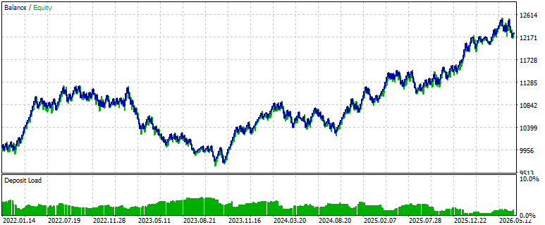
Fig. 9. Balance and equity over 436 trades, XAUUSD H1 from January 2022 to August 2026, at a 512-bar window and a target of one cycle amplitude

The tester puts numbers on that curve: 436 trades for a net 2240.27 on a 10000 deposit, a profit factor of 1.15, 64.22% of trades profitable, an average win of 61.27 against an average loss of 95.61, and a maximum balance drawdown of 1491.76, or 13.31%. Winning two trades in three while the average loss is half again the average win is what a near target and a wide stop look like from the account's side. It is also a curve that goes up, which is the kind of result that gets published without the test that comes next.

Now the honest part. A balance curve on its own says almost nothing about whether the signal knows anything, so the strategy carries a diagnostic input that takes the opposite of every signal and changes nothing else. If following loses and fading wins by a similar amount, the signal carries real information with the wrong sign; if both lose by about the cost of trading, it carries none.

Run	Following the signal	Fading the signal	Trades
XAUUSD H1, 2022 to 2026	12240 (+22.4%)	6060 (-39.4%)	436/436
XAUUSD D1, 2016 to 2026	10506 (+5.1%)	9182 (-8.2%)	47/47

Following beats fading by 61.8 percentage points on the hourly chart and by 13.2 on the daily, on the same signals in each pair. That asymmetry, rather than the balance curve above it, is the result worth reporting, and it is also the whole of the claim. These are two paired runs on one instrument with no significance test behind the gap, and things other than the signal could produce it: the stop and target are not symmetric, so reversing an entry does not reverse the trade; the instrument trended over both periods; and both arms inherit the same spread and the same execution model. The reversal test rules out the laziest explanation for a rising curve. It does not establish an edge.

The daily row deserves a note. A 512-bar window on daily bars is two years of history, and the tester hands out only 314 bars before the test starts, so the first 202 bars produce no model at all and the EA says so in the log rather than silently doing nothing. Over 2022 to 2026 the same configuration reaches just 11 trades, which is why the row above starts in 2016, and even then ten and a half years yields only 47.

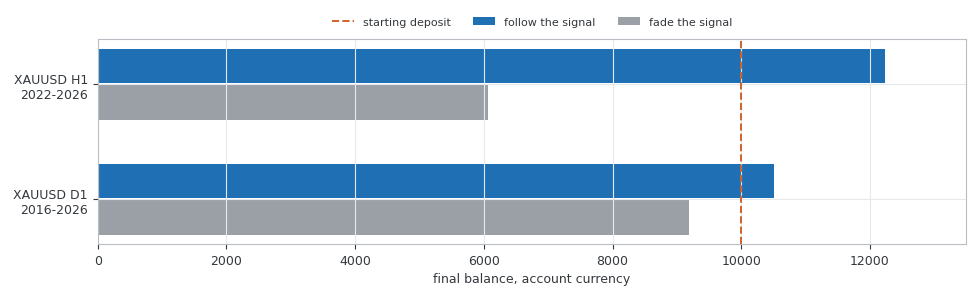
Fig. 10. Final balance from following the signal against fading it on gold, on the same trades in each pair

Important: this is a result for one instrument, one broker's history and one configuration, and it is offered as exactly that. Nothing here claims the strategy is profitable on other symbols, and anyone with the attached files should run it themselves first. Two limits matter inside that scope. There is no out-of-sample period, because this broker's gold hourly history begins in January 2021, and no walk-forward either, so nothing re-selects the settings as the data moves. And the outcome moves a long way on a setting unrelated to the trade logic: the same instrument, period and target on a 256-bar window returns 9474, a loss of 5.3%. Report the asymmetry. Do not read the 22% as an edge.

That is the evidence, stated in full. On gold, over this period and on both timeframes tested, following the decomposition's direction did better than fading it. With no out-of-sample period, no walk-forward, and an outcome that changes sign when the window moves from 512 to 256, that describes two backtests rather than demonstrating a robust signal. The strategy is one section of this article rather than its subject: the library, the causal boundary and the measurement of what hindsight buys are what have to stand on their own.

Conclusion

Variational Mode Decomposition now exists for MetaTrader 5 as a from-scratch library, agreeing with a deterministic reference to 1.29e-13 on the modes, wrapped in a causal boundary tested by sabotage rather than asserted, and reported alongside the numbers that say when to distrust it.

What was built:

• A radix-2 transform and centered-spectrum shift, checked against a direct O(N^2) transform, against closed forms, and against Parseval's identity and linearity.
• The ADMM solver, in two rolling rows rather than a full iteration history, matching the Python reference to 1.29e-13 on the modes and taking the same number of iterations on all eleven exported test cases.
• A data layer that owns the causal boundary, log transform, mean removal and power-of-two window, tested by overwriting the future and demanding an unchanged answer.
• A result type that carries convergence, unexplained energy and mode separation, so a bad solve can be refused instead of plotted.
• An indicator whose every plotted point is computed once from a window ending at its own bar, with an external script that reproduces those points independently.
• A strategy whose stop comes from the noise width, target from the traded mode's amplitude and holding time from that mode's half period, with a diagnostic that separates a real signal from a spread bleed.
• A measurement of what a batch decomposition adds, on three symbol and timeframe combinations against matched random walks.

The measurement is the part worth carrying away. On the three combinations looked at, a batch VMD chart is not a slightly optimistic version of the causal one: it points the other way on roughly a quarter to a third of bars, and a volatility-matched random walk drifts by a comparable amount. That is a result about these series rather than about markets in general, and not evidence about how any other decomposition behaves. It is a reason to run the same test before believing the picture such an indicator draws.

#	Filename	Type	Description
1	VMD.mqh	Include	Facade CVMD: runs one causal decomposition and exposes it by frequency rank, plus the amplitude, half period, noise width and regime readings
2	VMDData.mqh	Include	The causal boundary: bars to log prices to a mean-centered power-of-two window, with bar provenance
3	VMDTransform.mqh	Include	Radix-2 fast Fourier transform and the even-length centered-spectrum shift
4	VMDCore.mqh	Include	The ADMM solver: mirroring, analytic spectrum, Wiener filter, centroid and dual ascent over two rolling rows
5	VMDResult.mqh	Include	SVMDResult: the modes and frequencies plus convergence, unexplained energy and mode separation
6	VMD_Test_Transform.mq5	Script	Transform tests against a direct transform, closed forms, identities and input contracts
7	VMD_Test_Core.mq5	Script	Solver tests: planted tone recovery, residual bounds, convergence over a batch, mode separation and cost
8	VMD_Test_Facade.mq5	Script	Data layer and facade tests, including the causality-by-sabotage check
9	VMD_Export_ForCrosscheck.mq5	Script	Exports eleven configurations for the Python comparison, at full double precision
10	VMD_Scan_Market.mq5	Script	The repaint study: drift by bar age, endpoint profile, batch against causal, stability and the random-walk nulls
11	VMD_Verify_Indicator.mq5	Script	Drives the indicator through iCustom and reproduces its plotted points independently
12	VMD_Decomposition.mq5	Indicator	Causal denoised line, trend mode and ordinary-move band, with a panel carrying the modes and the solve verdict
13	VMD_Cycle_EA.mq5	Expert	Trades the oscillatory mode with stop, target, holding time and size all derived from the decomposition
14	vmd_prototype.py	Python	The restructured blueprint the MQL5 solver was written from, with its own self-test
15	vmd_crosscheck.py	Python	Compares the MQL5 export against the reference implementation and against the blueprint
16	MQL5.zip	Archive	Archive with all project files in their subfolders; unpack it into the terminal data directory and every file lands in its required location