Surrogate Data Testing: A Null Model for Any Statistic, and Why Shuffling Bars Is Not One

MetaTrader 5 — Trading | 13 October 2026, 15:04

176

Hammad Dilber

Introduction

Suppose your indicator reports a determinism of 0.73, or a persistence entropy of 1.42, or a time reversal asymmetry of -0.31. The number is real and the code is correct, yet the reading is uninterpretable, because nothing in the calculation tells you what that statistic would have produced on a series with no structure worth finding. Without that comparison a reading is a number, not a result.

The standard answer is a null model: generate many synthetic series sharing everything with your data except the thing you claim to have found, score the statistic on each, and see where the real reading lands among them. The difficulty is all in "share everything except". Get that wrong and the test answers a question nobody asked.

MQL5 already has permutation testing. Two articles cover it, both aimed at strategy results: Monte Carlo Permutation Tests in MetaTrader 5 permutes ticks, and Permuting price bars in MQL5 permutes bars, and both ask whether a backtest could have arisen by luck. That is a sound question about a P&L curve. It is usually the wrong question about an indicator, for a mechanical rather than philosophical reason. Shuffling bars destroys arrival order and, with it, the autocorrelation almost every technical indicator uses. A shuffled null therefore asks, "Is the indicator reading anything at all?" That is the right question for an indicator whose claim does not involve time ordering, and the wrong one for the majority that do. For those the relevant question is, "Is it reading anything beyond the linear correlation present in any trending or mean-reverting series?"

The difference is visible in one picture. The chart below takes 300 daily gold bars, converts them to absolute log returns, and plots the autocorrelation of the data against two candidate nulls. Absolute returns are used because raw gold returns have little linear structure (mean absolute autocorrelation over lags 1 to 10 is 0.064 against a noise band of 0.115), while absolute values exhibit volatility clustering, which is what a volatility statistic reads.

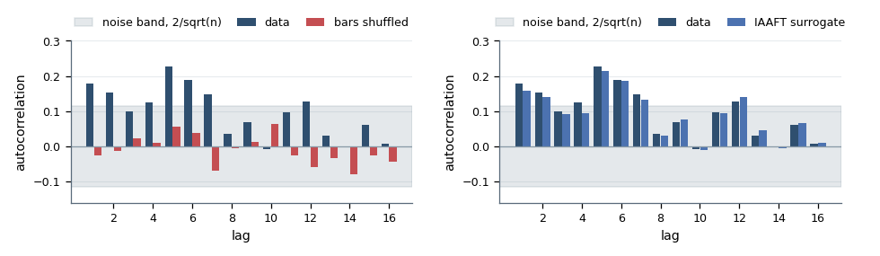
Two bar charts comparing the autocorrelation of the data with a bar-shuffled version and with an IAAFT surrogate

Fig. 1. Shuffling the bars collapses the autocorrelation into the noise band, while a surrogate reproduces it lag by lag

Mean absolute autocorrelation over the first sixteen lags: data 0.098, bar shuffled 0.036, surrogate 0.094. The shuffle removed the very structure the test should have held fixed. A statistic that reads volatility clustering will separate the data from a shuffled null every time, and the separation says nothing except that volatility clusters, which everybody knew. Note that this picture is drawn on absolute returns, where that clustering lives. The market tests later run on log returns themselves, whose linear structure is far weaker, so the picture motivates the choice of null rather than standing behind those findings.

A surrogate is the alternative: a synthetic series built to hold fixed whatever features define the null being tested, while destroying everything else. The four methods below hold different things fixed, and none holds both the amplitude distribution and the power spectrum exactly, a tension this article measures rather than hides. If your statistic reads the same on surrogates as it does on the data, then whatever it is detecting is already in the features that were held fixed, and the reading carries no further information. If it separates cleanly, you have evidence against that particular null, and which null it was decides what the evidence means. That is the test this article builds, in MQL5, with no external dependency.

What the test reads on real bars

Here is the finished library pointed at 512 daily gold log returns, running four statistics against four different null models, with 99 surrogates behind every cell.

[2] every statistic against every null
       99 surrogates, alpha 0.050, p floor 0.0200 two-tailed / 0.0100 one-tailed
       statistic        null      observed     null mean        sd        z       p
       trev(1)         FT       +0.077879    +0.010151  0.107531    +0.63  0.5400
                       AAFT     +0.077879    +0.017128  0.187362    +0.32  0.7400
                       IAAFT    +0.077879    +0.030893  0.230827    +0.20  0.8400
                       BLOCK    +0.077879    +0.083546  0.338389    -0.02  1.0000
       trev(3)         FT       +0.035350    -0.001607  0.080693    +0.46  0.6200
                       AAFT     +0.035350    -0.030679  0.214802    +0.31  0.8000
                       IAAFT    +0.035350    +0.020299  0.199194    +0.08  0.9200
                       BLOCK    +0.035350    +0.010591  0.221273    +0.11  0.8200
       prederr         FT       +1.088484    +1.116320  0.023250    -1.20  0.1600
                       AAFT     +1.088484    +1.120495  0.024695    -1.30  0.1200
                       IAAFT    +1.088484    +1.115241  0.023930    -1.12  0.1500
                       BLOCK    +1.088484    +1.022617  0.042075    +1.57  0.9600
       acf(1)          FT       +0.029230    +0.030134  0.002210    -0.41  0.4200
                       AAFT     +0.029230    +0.023496  0.016482    +0.35  0.6800
                       IAAFT    +0.029230    +0.029885  0.001600    -0.41  0.5600
                       BLOCK    +0.029230    +0.020167  0.053210    +0.17  0.8600
       ---
       0 of 16 cells cleared alpha 0.050

Zero of sixteen cells clear a significance of 0.05. The closest is the prediction error against the AAFT null at 0.1200, more than twice the threshold, and the largest distance anywhere in the table is 1.57 standard deviations. Nothing in this window separates gold's daily returns from any of the four nulls these rows were scored against, which between them cover a linear Gaussian process, a static transform of one, and short-range dependence with no spectral model at all.

A result of "nothing here" is only worth reading if the machinery could have said otherwise, so the scan runs a control on the same window whose correct answer is known before the run starts.

[3] the negative control
       circular acf(1) vs FT   observed +0.030282537   null sd 4.357e-17   p 1.0000
       CORRECT - phase randomization cannot move this statistic, and the
       test correctly refuses to separate what it cannot move.

The circular autocorrelation is fixed by the power spectrum, and phase randomization preserves that spectrum exactly, so every surrogate must score precisely what the data scores. The null's standard deviation is 4.4e-17, floating point noise and not a distribution at all, and the test returns p = 1.0000. A test that refuses to separate what it provably cannot separate is one whose machinery is working for this statistic against this null. That is one invariant holding, not a warrant covering every statistic and null in the table above.

Between those two extremes sits the thing a p-value actually summarizes. The next chart shows the null distribution behind a single cell, for a deterministic chaotic map on the left and for the real gold window on the right.

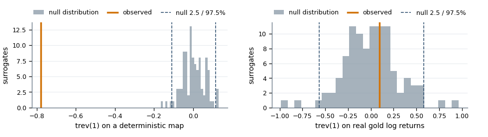
Two histograms of surrogate statistic values with the observed value marked on each

Fig. 2. The same statistic against the same null model, once on a deterministic map and once on real bars

On the left the observation sits far outside every surrogate it was compared against. On the right it sits in the middle of the pile. Both pictures are the same calculation; only the data changed. That is what this article delivers. The rest explains how.

What a surrogate has to preserve

A surrogate must be indistinguishable from the data under the null hypothesis and different from it under the alternative, which turns into two target constraints. The first is the amplitude distribution: the surrogate should contain the values the data contains, so no statistic can separate the two by reading the size of the moves. The second is the power spectrum, which by the Wiener-Khinchin theorem is the same thing as the autocorrelation function.

A permutation test and a surrogate test are often spoken of as one thing, and they answer different questions. A permutation test has two series and breaks the correspondence between them, which is right when the claim is that one relates to the other. A surrogate test has one series and no pairing to break, so it builds its comparison from that series alone, holding the two constraints above fixed. The constructions are opposites: a permutation destroys time ordering, while a spectral surrogate keeps the linear correlation structure and destroys only what is left. Reach for the first when testing a relationship, the second when testing a property of one series.

Those two constraints pull against each other, and the four methods in this library are four answers to that tension.

//+------------------------------------------------------------------+
//| Which null a surrogate is drawn from                             |
//|                                                                  |
//|  These are not four qualities of the same thing. They are four   |
//|  different NULL HYPOTHESES, and choosing one is choosing what    |
//|  "by chance" is allowed to mean.                                 |
//+------------------------------------------------------------------+
enum ENUM_SURROGATE_METHOD
  {
   SURROGATE_FT    = 0,    // linear Gaussian process
   SURROGATE_AAFT  = 1,    // static monotone transform of one
   SURROGATE_IAAFT = 2,    // the same, with the spectrum iterated back in
   SURROGATE_BLOCK = 3     // short-range dependence, no spectral model at all
  };

The comment is doing real work: these are four different null hypotheses rather than four qualities of one thing, and choosing one is choosing what "by chance" is permitted to mean. FT asks whether the data could be a linear Gaussian process. AAFT and IAAFT ask whether it could be a static, order-preserving transform of one, which is a strictly wider and more realistic hypothesis for price data. BLOCK abandons the spectral model entirely and asks only whether short-range dependence explains the reading; at the shipped setting it is the Politis-Romano stationary bootstrap with geometric block lengths of mean 10, so its null is specifically "dependence reaching about ten bars", and a different mean block length is a different null.

FT carries a scope limit the other three do not. The size measurement below shows it is usable only where the amplitude distribution is near Gaussian, so on every heavy-tailed series in this article its rows are controls and never results.

The chart below shows what survives each construction, computed on the same 256 real gold returns.

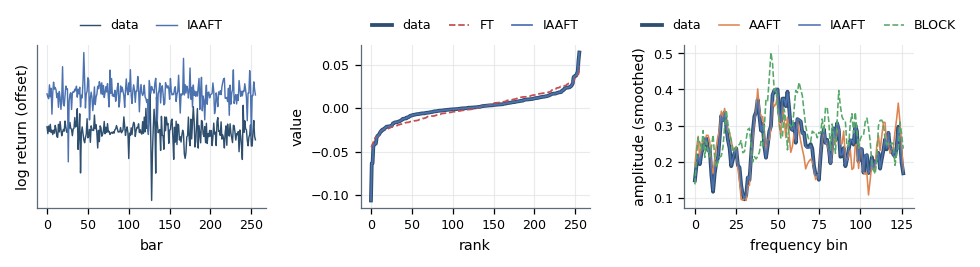
Three panels showing a series and its surrogate, sorted values, and smoothed power spectra

Fig. 3. The left panel is one surrogate beside its data, the middle panel is the amplitude constraint, and the right panel is the spectral constraint

In the middle panel the IAAFT curve lies exactly on the data's, because an IAAFT surrogate is a permutation of the data and its sorted values are identical to the last bit. The FT curve departs at both ends: phase randomization sums many independently phased sinusoids, so the result is Gaussian whatever it was built from and the extreme moves are pulled in. In the right panel the two rank-based methods track the data's spectrum closely while the bootstrap does not, which is what a method with no spectral model should look like.

Carrying a method that fails differently is not redundancy. A finding that survives both a spectral null and a bootstrap null is standing on two different sets of assumptions, and a finding that survives only one of them has told you precisely which assumption it needs. The two tests are not statistically independent, since they score the same statistic on the same series, so surviving both is not two confirmations and their p-values cannot be pooled as though it were.

A transform that accepts any length

Every spectral surrogate is a transform, an edit in the frequency domain, and a transform back, so the FFT is the engine the whole library runs on. A textbook radix-2 kernel accepts only powers of two, and both usual workarounds are wrong here: zero padding changes the spectrum, the one thing a surrogate must reproduce exactly, and snapping the length down discards up to half the series, so the null answers a different question.

Bluestein's chirp-z algorithm removes the choice. It rewrites a transform of any length as a convolution, which a radix-2 kernel can perform, at the cost of one padded transform. The dispatch is the only place a caller ever needs to think about it.

//+------------------------------------------------------------------+
//| A DFT of any length: radix-2 when it can, Bluestein otherwise    |
//|                                                                  |
//|  The inverse of a non-radix-2 length goes through the identity   |
//|  IDFT(X) = conj(DFT(conj(X))) / n, so only the forward chirp     |
//|  path ever runs and only one kernel is ever cached.              |
//+------------------------------------------------------------------+
bool CSurrogateTransform::DFT(double &re[], double &im[], const bool inverse)
  {
   int n = ArraySize(re);
   if(n != ArraySize(im))
     {
      Print("SurrogateTransform::DFT - real and imaginary parts differ in length");
      return(false);
     }
   if(n < 1)
      return(false);
   if(n == 1)
      return(true);
 
   if(IsPow2(n))
      return(FFT(re, im, inverse));
 
   if(!inverse)
      return(Bluestein(re, im));
 
   for(int i = 0; i < n; i++)
      im[i] = -im[i];
   if(!Bluestein(re, im))
      return(false);
 
   double invn = 1.0 / (double)n;
   for(int i = 0; i < n; i++)
     {
      re[i] =  re[i] * invn;
      im[i] = -im[i] * invn;
     }
   return(true);
  }

Two details in that function are load bearing. The chirp path is forward only: the kernel is cached already transformed, and conjugating a transformed kernel is not the same operation as conjugating it beforehand, which yields a result of the right shape that is simply wrong. Reaching the inverse through the identity in the header means one kernel is ever built and no second sign convention can drift out of step.

The second is the cost. Measured with GetMicrosecondCount, minimum of five runs, the radix-2 kernel takes 6.0, 13.8 and 32.0 microseconds at lengths 256, 512 and 1024, while the chirp path takes 32.4, 66.9 and 143.3 microseconds at the adjacent lengths 250, 500 and 1000. About five times as much, which is the price of not having to lie about the window length, and it is worth paying.

Important: the twiddle factors are cached per length rather than evaluated inside every butterfly. One IAAFT surrogate is a few hundred transforms and a null distribution is hundreds of them, so calling a cosine and a sine inside the inner loop spends nearly all the time in trigonometry.

Building the four nulls

Phase randomization is the primitive the two spectral methods are built from. The magnitude of each Fourier coefficient is kept, its phase is replaced by a uniform draw, and the series is transformed back.

//+------------------------------------------------------------------+
//| Give every free Fourier coefficient a uniform phase              |
//|                                                                  |
//|  Conjugate symmetry is enforced explicitly: k and n-k are set    |
//|  from one draw AND one shared amplitude, so rounding cannot      |
//|  break the symmetry. The constant term is the series mean;       |
//|  on an even length Nyquist is its own conjugate.                 |
//+------------------------------------------------------------------+
bool CSurrogateGenerator::RandomizePhases(const int n, CSurrogateRandom &rng)
  {
   for(int i = 0; i < n; i++)
      m_amp[i] = MathSqrt(m_re[i] * m_re[i] + m_im[i] * m_im[i]);
 
   int half = (n - 1) / 2;
   for(int k = 1; k <= half; k++)
     {
      double phi = 2.0 * M_PI * rng.Uniform();
      double cr  = MathCos(phi);
      double ci  = MathSin(phi);
 
      //--- a real series has |X[k]| = |X[n-k]|, but the two bins reach it
      //--- down different arithmetic paths; average them and use the one
      //--- value for both, so the pair is conjugate to the last bit
      double a = 0.5 * (m_amp[k] + m_amp[n - k]);
 
      m_re[k] = a * cr;
      m_im[k] = a * ci;
 
      m_re[n - k] =  a * cr;
      m_im[n - k] = -a * ci;
     }
 
   m_im[0] = 0.0;
   if((n % 2) == 0)
      m_im[n / 2] = 0.0;
   return(true);
  }

Coefficients k and n-k are set from one draw and one shared amplitude, each the conjugate of the other, which is what makes the inverse transform real rather than complex. Two coefficients are left alone: the constant term, because it is the series mean, and on an even length Nyquist, because it is its own conjugate and has no free phase to give away.

AAFT wraps that primitive in two rank remaps: the data is replaced by Gaussian values of the same ranking, the Gaussian copy is phase randomized, and the original values are put back by rank. The output is an exact permutation of the data, so the amplitude constraint holds perfectly, while the two remaps have bent the spectrum. IAAFT alternates the two constraints until neither improves.

//+------------------------------------------------------------------+
//| IAAFT: impose the spectrum, impose the distribution, repeat      |
//|                                                                  |
//|  The loop stops when the RANKING repeats, since the next pass    |
//|  reproduces the identical array. On heavy tails it stops with    |
//|  the spectrum still off: a fixed point of THIS scheme, which a   |
//|  different scheme might improve on. Ends on the distribution.    |
//+------------------------------------------------------------------+
bool CSurrogateGenerator::GenIAAFT(const double &x[], const int n, CSurrogateRandom &rng,
                                   double &out[])
  {
   m_sort.SortedCopy(x, n, m_sorted);
   if(!m_fft.Spectrum(x, n, m_amp))
      return(false);
 
   for(int i = 0; i < n; i++)
      out[i] = x[i];
   rng.Shuffle(out, n);
 
   bool havePrev = false;
   m_lastConverged = false;
 
   for(int it = 1; it <= m_maxIter; it++)
     {
      m_lastIter = it;
 
      //--- impose the target spectrum, keeping the current phases
      for(int i = 0; i < n; i++)
        {
         m_re[i] = out[i];
         m_im[i] = 0.0;
        }
      if(!m_fft.DFT(m_re, m_im, false))
         return(false);
 
      for(int k = 0; k < n; k++)
        {
         double mag = MathSqrt(m_re[k] * m_re[k] + m_im[k] * m_im[k]);
         if(mag > 0.0)
           {
            double s = m_amp[k] / mag;
            m_re[k] *= s;
            m_im[k] *= s;
           }
         else
           {
            m_re[k] = m_amp[k];
            m_im[k] = 0.0;
           }
        }
      if(!m_fft.DFT(m_re, m_im, true))
         return(false);
 
      for(int i = 0; i < n; i++)
         m_work[i] = m_re[i];
 
      //--- impose the target distribution
      m_sort.RankAndRemap(m_work, n, m_sorted, m_ranks, out);
 
      if(havePrev && m_sort.SameRanks(m_ranks, m_prev, n))
        {
         m_lastConverged = true;
         break;
        }
      for(int i = 0; i < n; i++)
         m_prev[i] = m_ranks[i];
      havePrev = true;
     }
 
   m_lastSpecErr = SpectralError(out, n);
   return(true);
  }

The stopping rule is the part worth studying. The loop ends when the ranking reaches a fixed point, not when an error falls below a threshold. Once the ranking repeats, the next iteration reproduces the identical array and there is nothing further to gain. On heavy-tailed data that fixed point is reached with the spectrum still visibly off, and raising the iteration cap changes nothing.

What that establishes is a fixed point of this particular alternating projection, which is weaker than the two constraints being mathematically incompatible: another scheme might reach a better compromise, and nothing measured here rules that out. LastSpectralError reports how far off it settled, and every consumer prints it.

Note also that the loop always ends on the distribution step. The surrogate is therefore an exact permutation of the data and only the spectrum is approximate. Stopping on the other side would leave a series that is not comparable to the data at all under any statistic that reads amplitudes.

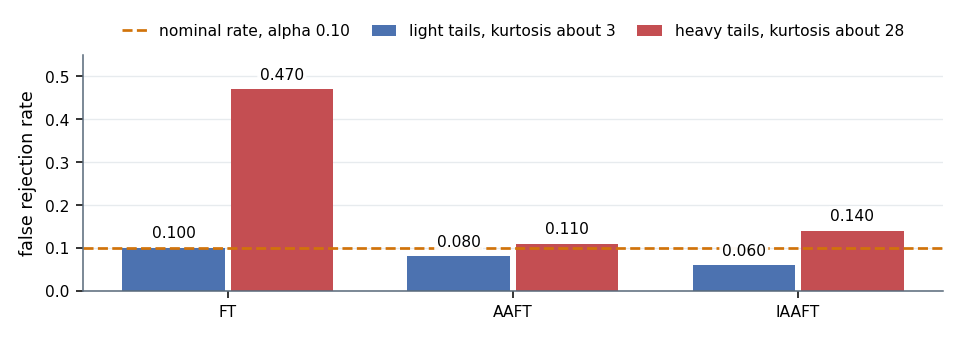
Grouped bar chart of rejection rates for FT, AAFT and IAAFT against a nominal rate line

Fig. 4. Every rejection in this chart is false by construction, because both test processes are linear Gaussian underneath

That picture is the measurement the choice of method rests on, from the library's own test script. Two processes are used, both linear Gaussian underneath: a plain AR(1), and the cube of one, which is a static order-preserving transform of a linear process and therefore squarely inside the null AAFT and IAAFT were built for. Every rejection is a false positive.

[3] size under H0 - the rate at which a linear process is rejected
       100 trials, 19 surrogates, n=256, alpha 0.10
       method   tails    rejected      rate   Wilson 95%
       FT       light      10/100     0.100   [0.055, 0.174]
       FT       heavy      47/100     0.470   [0.375, 0.567]
       AAFT     light       8/100     0.080   [0.041, 0.150]
       AAFT     heavy      11/100     0.110   [0.063, 0.186]
       IAAFT    light       6/100     0.060   [0.028, 0.125]
       IAAFT    heavy      14/100     0.140   [0.085, 0.221]
  PASS  IAAFT is consistent with nominal, light tails   0.060
  PASS  AAFT is consistent with nominal, light tails   0.080
  PASS  FT is consistent with nominal, light tails   0.100
  PASS  FT is badly oversized on heavy tails   0.470 against a nominal 0.10
  PASS  IAAFT is far better there   IAAFT 0.140 vs FT 0.470
  PASS  and so is AAFT   AAFT 0.110 vs FT 0.470
  PASS  IAAFT is not separable from nominal, heavy tails   0.140

Read those rates with their intervals rather than as a ranking. At 100 trials a measured 0.060 carries a 95% Wilson interval of 0.028 to 0.125 and a measured 0.100 carries 0.055 to 0.174, so the three light-tail rates cannot be separated from each other or from the nominal 0.10, and the apparent ordering among them is sampling noise. What the study does resolve is the heavy-tail gap: FT at 0.470 with an interval of 0.375 to 0.567 against IAAFT at 0.140 with 0.085 to 0.221. AAFT against IAAFT on heavy tails is not resolved either, and 19 surrogates per trial makes each individual p-value coarse on top of that.

FT rejects a linear process 47 times out of 100 when the tails are heavy, against a nominal rate of 0.10. The mechanism is the one visible in Fig. 3: FT surrogates are Gaussian by construction, so on a heavy-tailed series they differ from the data in distribution as well as in dynamics, and any statistic that reads the tails separates them for a reason that has nothing to do with the dynamics being tested.

The log returns measured for this article are heavy-tailed: a set of major pairs, gold and an index on daily bars read kurtosis between 8 and 12, and the two windows used below read 11.7 and 18.6. That describes these series rather than stating a law about markets, and the estimate is itself unstable, because a fourth moment over 256 to 512 points is dominated by a handful of the largest moves.

This is why the library ships IAAFT as its default and prints a warning whenever kurtosis exceeds 6. That threshold is a heuristic trigger placed between the near-Gaussian and heavy-tailed cases measured above, not a test with a calibrated level. It is also why the FT row stays in the scan output: read as a control it shows what a badly matched null looks like, and read as a result it would be an error.

The price of AAFT and IAAFT is that neither reaches the target spectrum exactly, and how far they miss depends on the data.

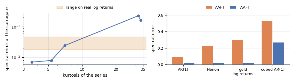
A line plot of spectral error versus kurtosis and a grouped bar chart comparing AAFT with IAAFT

Fig. 5. The miss grows with the weight of the tails, and IAAFT beats AAFT on every series tested

On a near Gaussian series IAAFT settles at a spectral error around 7e-03. By kurtosis 33 it settles at 1.6e-01, more than twenty times worse, and raising the iteration cap changes nothing because the ranking has stopped moving. On real gold log returns the error lands between 1.8e-02 and 4.7e-02. The right panel shows the same quantity for both rank-based methods on the four series the export covers: IAAFT is better everywhere, by a factor of seven on the AR(1) and twenty two on the real returns.

Do not read a large spectral error as a broken surrogate. Read it as a warning that on this series the two constraints could not both be satisfied, which means the hypothesis actually under test is an approximation of the stated one: AAFT and IAAFT test "a static transform of a linear process whose spectrum is close to this one", and the printed number is how close. On a near-Gaussian series that gap is negligible; at kurtosis 33 it is not, and a reading there has to be quoted with its spectral error beside it. The number is reported per surrogate for exactly that reason.

Any statistic, including one of your own

The test does not care what the number means. It needs one operation: given a series, return a number. That is why the statistic is an interface rather than a fixed menu.

//+------------------------------------------------------------------+
//| CSurrogateStatistic - the thing being tested                     |
//|                                                                  |
//|  A surrogate test needs exactly one operation: given a series,   |
//|  return a number. Tail() carries the DEFAULT direction for the   |
//|  statistic; override it when the hypothesis asks for another.    |
//|  Evaluate returns EMPTY_VALUE when the statistic is undefined.   |
//+------------------------------------------------------------------+
class CSurrogateStatistic
  {
public:
   virtual          ~CSurrogateStatistic(void) {}
 
   virtual double    Evaluate(const double &x[], const int n) = 0;
   virtual string    Name(void) const { return("statistic"); }
   virtual ENUM_SURROGATE_TAIL Tail(void) const { return(SURROGATE_TAIL_TWO); }
  };

Three methods, only one of which is mandatory. Name exists so a result can identify itself in a log. Tail records which direction counts as evidence, and ships with the statistic because the usual answer follows from how the statistic is built: prediction error is evidence when low, time reversal asymmetry when far from zero either way.

A caller made to remember that for every statistic would eventually get it wrong, and the consequence is not a warning but a silently halved or doubled p-value. The direction is not always a property of the statistic alone, though, which is why Tail is virtual rather than fixed: a hypothesis that is genuinely one-sided where the default is two should override it, and gains the lower p-value floor by doing so.

The library ships four implementations. The canonical one is time reversal asymmetry.

//+------------------------------------------------------------------+
//| The normalized third moment of the lagged increment              |
//|                                                                  |
//|  Too few points, or a constant increment, leaves the ratio       |
//|  undefined rather than zero, so it returns EMPTY_VALUE and the   |
//|  null refuses the run instead of ranking a fabricated 0.0.       |
//+------------------------------------------------------------------+
double CStatTimeReversal::Evaluate(const double &x[], const int n)
  {
   if(n <= m_lag + 1)
      return(EMPTY_VALUE);
 
   double s2 = 0.0, s3 = 0.0;
   int    c  = 0;
   for(int t = m_lag; t < n; t++)
     {
      double d = x[t] - x[t - m_lag];
      s2 += d * d;
      s3 += d * d * d;
      c++;
     }
   if(c < 1)
      return(EMPTY_VALUE);
 
   double m2 = s2 / c;
   if(m2 <= 0.0)
      return(EMPTY_VALUE);
   double m3 = s3 / c;
   return(m3 / MathPow(m2, 1.5));
  }

The reason this statistic is canonical is worth stating exactly. A linear Gaussian process is time reversible: the series and its reverse share a distribution, so the lagged increment is symmetric and every odd moment of it is zero. The numerator is therefore zero in expectation for the entire null hypothesis at once, without needing to know anything about the process beyond its linearity. Markets are not time reversible, since a crash and a recovery do not have the same shape, so this statistic has a real chance of reading something on price data. Whether it does is a measurement, reported below.

The other three are a lag-k autocorrelation, a circular autocorrelation, and a locally constant prediction error that embeds the series and predicts each point from its nearest neighbors elsewhere in the record. The two autocorrelations look redundant and are not, which turns out to be the sharpest practical lesson in the library.

Series length	Ordinary autocorrelation	Circular autocorrelation	Nominal rate
128	0.133	0.067	0.10
256	0.283	0.017	0.10
512	0.183	0.100	0.10

Those are false rejection rates on a pure AR(1) against an IAAFT null, 60 trials per cell, every rejection false by construction. The power spectrum pins down the circular autocorrelation, which wraps the series round so the last point is followed by the first. The ordinary sample version drops that wrap-around term, so a spectral surrogate reproduces it only to order 1/n. That is not negligible, because what it must be small against is not the statistic but the null's own spread, and an IAAFT null here is extremely tight precisely because the spectrum is nearly preserved. Pair a statistic with a null that preserves it exactly and the test is exact; approximately, and the leftover term competes with the null's width.

Both statistics ship. The circular one is the negative control used in section 3, and the ordinary one is kept because it is what everybody actually computes, and a reader testing their own autocorrelation needs to see this behavior rather than be protected from it.

Using the library on your own statistic is three lines.

//+------------------------------------------------------------------+
//| Section 3: the negative control, on real bars                    |
//|                                                                  |
//|  The circular autocorrelation is preserved by FT to machine      |
//|  precision, so the only correct answer is p = 1.0000. On the     |
//|  real window it is a live check that the transform, the shuffle  |
//|  and the ranking are all still doing what they claim.            |
//+------------------------------------------------------------------+
void ReportControl(CSurrogate &S, const double &x[], const int n)
  {
   Print("[3] the negative control");
 
   CStatCircularAutocorrelation cacf(1);
   SSurrogateNull r;
   if(!S.Test(GetPointer(cacf), x, n, SURROGATE_FT, r))
     {
      Print("       the control could not be run");
      return;
     }
 
   PrintFormat("       circular acf(1) vs FT   observed %+.9f   null sd %.3e   p %.4f",
               r.observed, r.sd, r.pSelected);

Build the statistic, hand it a series with a method and a surrogate count, read the result. Subclass CSurrogateStatistic , return your own indicator's value from Evaluate , declare which tail is evidence, and the whole apparatus applies to it unchanged.

The null distribution, and the floor on what you can ask

With the surrogates built and the statistic scored, the remaining work is ranking the observation among the draws.

//--- ties count as "at least as extreme" on BOTH sides, to a relative
//--- tolerance: FT preserves the circular acf exactly, so a strict >=
   out.nGE = 0;
   out.nLE = 0;
   for(int i = 0; i < count; i++)
     {
      double tol = SURROGATE_TIE_EPS *
                   (MathAbs(m_draws[i]) + MathAbs(out.observed) + 1.0);
      if(m_draws[i] >= out.observed - tol)
         out.nGE++;
      if(m_draws[i] <= out.observed + tol)
         out.nLE++;
     }
 
   double denom = count + 1.0;
   out.pUpper = (1.0 + out.nGE) / denom;
   out.pLower = (1.0 + out.nLE) / denom;
   out.pTwo   = MathMin(1.0, 2.0 * MathMin(out.pUpper, out.pLower));
   out.pFloor = SurrogatePFloor(count, out.tail);
 
   switch(out.tail)
     {
      case SURROGATE_TAIL_UPPER:
         out.pSelected = out.pUpper;
         break;
      case SURROGATE_TAIL_LOWER:
         out.pSelected = out.pLower;
         break;
      default:
         out.pSelected = out.pTwo;
         break;
     }

The p-value counts the observation itself, giving (1 + number as extreme) / (count + 1) rather than a plain proportion. That is not conservatism for its own sake. Under the null the observation is exchangeable with the surrogates, so it belongs in the ranking, and leaving it out produces a p-value that can reach zero, which is a claim no finite number of draws can support.

Two properties of that calculation need stating plainly. Doubling the smaller side is the standard two-tailed rank p-value and it is exact only when the null distribution is symmetric; these nulls are empirical and need not be, so on a skewed null the doubled value is a convention rather than a statement about equally extreme outcomes. And the z column printed beside every p-value is a distance in units of the null's own spread, nothing more. Since that null can be skewed or long-tailed, z is descriptive rather than a parametric criterion, and the rank p-value next to it is the inference.

The tie tolerance is the other detail, and it closes a real hole. Some statistics are preserved by some surrogates exactly, the circular autocorrelation under FT being this library's example. A strict comparison then decides every such case on the last bit or two of a number carrying no information, the p-value comes out uniform, and the test rejects at its nominal rate on a statistic it cannot be measuring. Counting ties as "at least as extreme" on both sides is the standard permutation treatment and errs conservatively.

That leaves the question of what significance the run can reach at all, which is decided before any data is seen.

//+------------------------------------------------------------------+
//| The smallest p-value a surrogate count and a tail can produce    |
//|                                                                  |
//|  A one-sided p-value can reach 1/(count+1). A two-sided one is   |
//|  twice the smaller side, so it reaches only 2/(count+1).         |
//|  Measured: an observation beyond all 49 surrogates, nGE 49 and   |
//|  nLE 0, returns 0.0400 and never 0.0200.                         |
//+------------------------------------------------------------------+
double SurrogatePFloor(const int count, const ENUM_SURROGATE_TAIL tail)
  {
   if(count < 1)
      return(1.0);
   double f = (tail == SURROGATE_TAIL_TWO ? 2.0 : 1.0) / (count + 1.0);
   return(f > 1.0 ? 1.0 : f);
  }
 
//+------------------------------------------------------------------+
//| The smallest surrogate count that puts alpha within reach        |
//+------------------------------------------------------------------+
int SurrogateRequiredCount(const double alpha, const ENUM_SURROGATE_TAIL tail)
  {
   if(alpha <= 0.0 || alpha >= 1.0)
      return(0);
   return((int)MathCeil((tail == SURROGATE_TAIL_TWO ? 2.0 : 1.0) / alpha) - 1);
  }

A rank-based p-value cannot fall below a floor set by the number of surrogates, and that floor differs between one-sided and two-sided statistics. A one-sided p can reach 1/(count+1), the observation lying beyond every surrogate; a two-sided p is twice the smaller side, so it reaches only 2/(count+1). Quoting the one-sided number for a two-tailed statistic advertises a significance it cannot arithmetically produce.

Two decreasing curves with a horizontal significance line and markers at 19 and 39 surrogates

Fig. 6. Nineteen surrogates reach a significance of 0.05 one-tailed and only 0.10 two-tailed, so the same count answers the question two different ways

Three of the four statistics here are two-tailed. Run one with 19 surrogates and ask for a significance of 0.05, and the smallest p-value obtainable is 0.10, so nothing can clear the threshold however clean the separation. A report reading "cleared 0 of 30 windows" would then be arithmetic rather than a market reading, and the two are indistinguishable on the page.

The library refuses to let that pass silently. SurrogatePFloor and SurrogateRequiredCount both default to the two-tailed answer when a caller does not say which tail they mean, because it is the stricter. Every result carries its own floor computed from its own statistic's tail, and the scan prints both. The indicator warns at startup when the count cannot reach the requested significance, and ships with 39 surrogates rather than 19 for that reason.

Significance wanted	Surrogates, one-tailed	Surrogates, two-tailed
0.10	9	19
0.05	19	39
0.01	99	199
0.001	999	1999

A perfect separation lands exactly on the floor, which is what makes the floor a floor. The test suite asserts it directly: a chaotic map scored against 49 surrogates lies beyond every one of them, nGE 49 and nLE 0, and the two-tailed p comes back as 0.0400 rather than 0.0200.

Verification

A library whose entire output is a null distribution has an awkward verification problem: there is no external answer to compare against, because the answer is a distribution depending on a random stream. The usual reference packages are Python libraries with no build available on the target machine, so the cross-check had to be self-contained.

The solution is to share the random stream rather than merely match it. The library carries its own generator, splitmix64 into xorshift64*, both pure unsigned 64-bit arithmetic. MQL5's ulong wraps exactly the way Python's masked integers do, so one seed produces the same sequence in both languages, bit for bit. That turns the cross-check from a statistical comparison into an equality: the reference does not produce similar surrogates, it produces the same surrogates. What that equality establishes is that two implementations of one specification agree, which is reproducibility and not statistical validity. It cannot tell you the null model suits your question, or that the hypothesis is the one you meant to test; the size study is the part of this article that tests the method rather than the code.

Everything built on that stream is genuinely independent. The transform is checked against numpy's FFT and, separately, against the O(n^2) definition written longhand. The merge sort is checked against numpy's argsort, and every statistic is written from its definition on both sides. A set of invariants needs no reference at all: an FT surrogate must have the data's spectrum, an AAFT or IAAFT surrogate must be an exact permutation of the data, and a bootstrap surrogate must draw only values the data contains.

Level	Script	Result
Blueprint	surrogate_prototype.py	51 PASS, 0 FAIL
Transform	Surrogate_Test_Transform.mq5	120 PASS, 0 FAIL, worst error 2.0e-12
Generator	Surrogate_Test_Generator.mq5	80 PASS, 0 FAIL
Null	Surrogate_Test_Null.mq5	83 PASS, 0 FAIL
Cross-check	surrogate_crosscheck.py	129 PASS, 0 FAIL

The cross-check numbers are the ones worth quoting. The unsigned stream, the uniforms, the bounded integers and the geometric block lengths all reproduce at exactly zero error. An entire IAAFT surrogate, hundreds of transforms and sorts deep, comes back bit-identical on all four exported series including the real gold bars. The transform agrees with numpy to 3.4e-14, the statistics to 1.4e-14, and the null distributions to 1.4e-15.

To reproduce this yourself, run Surrogate_Export_ForCrosscheck.mq5 on any chart and then python surrogate_crosscheck.py . Run the export first: the cross-check reads a file the export writes, and comparing against a stale file will report differences that belong to the file rather than to the code.

What real markets read

The scan starts by describing the window it selected, because two of those numbers can invalidate everything below them.

[1] the window
       symbol            XAUUSDm PERIOD_D1
       input             log returns
       points            512
       kurtosis          11.68
       endpoint mismatch 0.027 sd
       note              512 points of log returns, window at offset 3086 of 3648 (endpoint mismatch 0.027 sd) [kurtosis 11.7 - heavy tails, FT surrogates are not valid here]

Kurtosis 11.68 says the tails are heavy, so the FT row is a control rather than a result. The endpoint mismatch of 0.027 standard deviations says the window's first and last values very nearly meet. That matters because the transform treats the window as one period of a periodic signal: if the two ends are far apart, the transform must represent a step discontinuity, and it does that with power spread across every frequency. That spread is already in the data's own spectrum, so the surrogates inherit it rather than suffering it alone. What differs is phase: the data keeps the alignment that concentrates the broadband power into one join, while a phase-randomized surrogate scatters it through the series.

SelectBestWindow slides the window over a search range and keeps the position whose ends meet most closely, which is the standard remedy and costs almost nothing. It is also a data-dependent choice the null distribution knows nothing about, and the window it lands on is a slightly different sample rather than the same sample measured better, so a selected reading is conditional on that selection and carries a bias this article does not quantify.

Section 3 already showed the headline: zero of sixteen cells cleared on gold, and on EURUSD H1 the same scan cleared two. The obvious reading is that something was found; the correct one is that sixteen tests at a threshold of 0.05 produce about one hit by luck. The way to tell them apart is to run the same test on a different window.

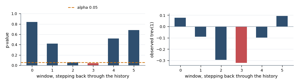
Two bar charts showing p-values and observed statistic values for six consecutive test windows

Fig. 7. One window clears the threshold and its five neighbors do not, while the observed statistic swings from positive to negative across them

[4] the same test on separate windows
       6 windows of 512 points, stepping back through the history
       statistic        window   observed        p (IAAFT)
       trev(1)             0    +0.077879     0.8400
                           1    -0.089936     0.4200
                           2    -0.295276     0.0600
                           3    -0.321093     0.0400  <= alpha
                           4    -0.097888     0.5200
                           5    +0.092803     0.6800
                       cleared alpha on 1 of 6 windows

Window 3 clears a significance of 0.05 at p = 0.0400. Its immediate neighbors read 0.0600 and 0.5200, and across the six windows the observed statistic swings from +0.0928 to -0.3211, which is a change of sign. Report window 3 on its own and you have discovered time irreversibility in gold. Report all six and the support for that is gone. Six windows cannot prove the reading was noise rather than a local effect only window 3 spanned; what they establish is that nothing here supports a claim about the series as a whole. A p-value from one window is one draw, and the scan exists to make that impossible to forget.

Across both symbols the full count is 48 window tests with 2 clearing, against the 2.4 that a threshold of 0.05 produces by itself, and never the same window twice.

Counting expected false positives is not a correction, so here is one. Applying the Benjamini-Hochberg procedure at a false discovery rate of 0.05 to the sixteen p-values in section 3 rejects nothing, which the raw table already said. Applied to the six windows above it also rejects nothing: window 3's 0.0400 would have to fall below 0.0083 to survive six comparisons, and it does not. That is the formal version of the reading given above.

The same arithmetic exposes a limit of the run itself. A two-tailed p-value cannot fall below 2/(count+1), so this scan's floor is 0.0200 at 99 surrogates and 0.0400 at 49. A corrected threshold across sixteen tests is 0.0031, and across the 48-test family 0.0010. Both sit below both floors, which means no cell anywhere in this scan could have produced a multiplicity-corrected rejection however cleanly it separated. Reaching them needs 639 surrogates for the sixteen-cell table and 1,919 for the 48-test family, by the same SurrogateRequiredCount arithmetic the library exposes. Everything above is therefore a screening result, and a confirmatory run must be budgeted against the corrected floor from the start.

One trap deserves its own measurement rather than a warning in a comment, because the number it produces is exactly the kind that looks like a discovery.

//+------------------------------------------------------------------+
//| What to feed the test                                            |
//+------------------------------------------------------------------+
enum ENUM_SURROGATE_INPUT
  {
   SURROGATE_INPUT_LOGRET = 0,   // log returns - the default, and the correct one
   SURROGATE_INPUT_DIFF   = 1,   // first differences
   SURROGATE_INPUT_RAW    = 2    // the level itself; see the warning below
  };

Run the identical test on raw closing prices and time reversal asymmetry reads p = 0.0200 on gold daily bars and p = 0.0200 on EURUSD H1, significant on both, with endpoint mismatches of 2.63 and 3.66 standard deviations. Nothing has been discovered. A trending price is not stationary, so a phase-randomized version of it is not a null being tested, it is a different random walk compared to this one. CSurrogateData defaults to log returns for that reason, and warns in its note rather than refusing, so a reader can run the wrong thing deliberately and see what it produces.

Log returns remove the trend, and they do not deliver stationarity. Regime shifts and slow drift in volatility survive the transformation, while the spectrum and the amplitude distribution a surrogate copies are both global over the window. A window spanning two volatility regimes therefore gets a null built from their average, which no local structure in either regime has to match. Nothing in this article tests for that, and it qualifies every reading here.

The last practical matter is cost, and there is no general rule because which half dominates flips with the pair you choose. Measured on 512 real gold returns: FT costs 88 microseconds per surrogate, AAFT 429, IAAFT 3907 and BLOCK 3, while time reversal asymmetry costs 0.811 microseconds per evaluation and the prediction error 2385. The scan times each pair together in one pass, and the verdict flips across the three it reports: FT with prediction error is statistic bound by a factor of 40, IAAFT with prediction error surrogate bound by 1.8, and IAAFT with time reversal asymmetry surrogate bound by 5192. Budget the pair you intend to run.

The indicator

Surrogate_Nonlinearity.mq5 plots a statistic in a subwindow, inside the shaded band its null occupies. The band is not decoration: a line at 0.34 means nothing on its own, and only its position relative to the band carries information. It is drawn as a filled region rather than two boundary lines because the reading is a containment question, and the eye should answer "inside or outside" without working out which line is which.

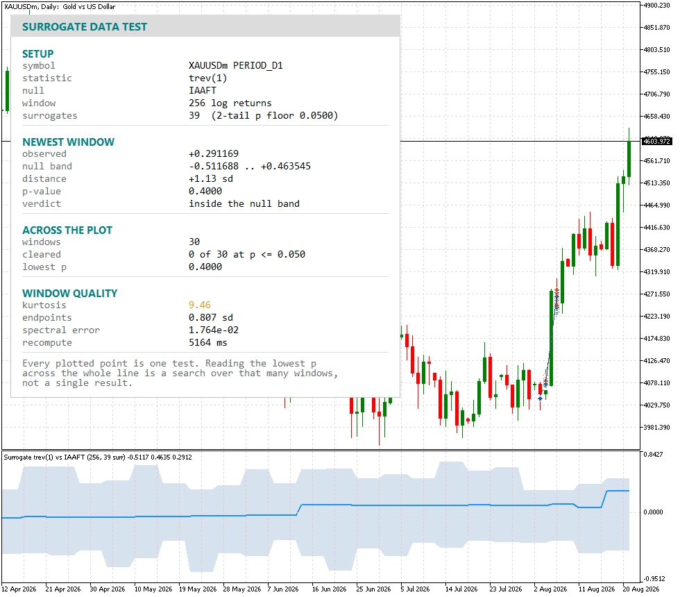
A MetaTrader chart with the statistic and its null band in a subwindow and a summary panel

Fig. 8. The statistic stays inside its null band all the way across, and the panel flags this window's kurtosis in orange

Three properties of the display are deliberate. The line is a staircase: a full test costs seconds, so a window is computed every InpStep bars and held in between, and interpolating would produce a drawing rather than a measurement. The recompute happens once per completed bar, never per tick. And the forming bar repeats the last closed one, since a null built partly from a value still moving is not reproducible tick to tick.

One property of the line matters more than those and is easy to misread. Consecutive windows overlap almost completely: at the shipped settings a window is 256 points and the step is 5, so neighboring readings share 251 of their 256 points. Thirty plotted windows are therefore nowhere near thirty independent tests, and a run of them clearing together is one finding smeared across a moving window rather than thirty confirmations. The stability check above steps by half a window instead, which is why its six readings are worth comparing and thirty adjacent ones are not.

Cost governs the defaults. On daily gold, 150 plotted bars at a step of 5 with an IAAFT null and 39 surrogates cost between 1.5 and 2.4 seconds per recompute over 34 measured passes of an otherwise idle terminal, and between 3.5 and 5.2 over the six taken while a screen capture shared the thread, which is why the panel in Fig. 8 reads 5164 ms. The same display with an FT null costs 33 milliseconds, which states plainly where the time goes. InpHistoryBars and InpStep are the two levers, and raising the first without lowering the second makes the first load noticeably slow.

The panel reports the newest window's observation, its null band, its distance in standard deviations, the p-value with its floor, and the two window quality figures that decide whether any of it is trustworthy. Kurtosis reads 9.46 and is colored orange, the heavy-tailed regime where an FT null would be unusable, so this window's reading depends on IAAFT having been chosen. The endpoint mismatch reads 0.807 standard deviations and is not flagged. Neither number invalidates a reading alone, and both are the first things to check before believing one.

The p-value is marked in red only when the reading actually clears the requested significance, and the floor is printed beside the surrogate count so a permanently unreachable threshold is visible rather than mysterious.

Conclusion

Surrogate data testing turns a statistic into a claim that can be falsified. The library attached here builds four null models from your own bars, scores any statistic you supply, and reports every number that could make the result untrustworthy: the surrogate count, the reachable floor, the spectral error, the kurtosis and the endpoint mismatch.

What was built:

A radix-2 FFT with cached twiddle factors, plus Bluestein's algorithm so that any window length is transformable without padding or truncation.
Four surrogate generators: Fourier phase randomization, amplitude adjusted Fourier transform, its iterative refinement, and the Politis-Romano stationary bootstrap.
A statistic interface with four implementations, including a negative control whose correct answer is known before any run.
A null distribution with a tail-aware p-value floor, a tie tolerance, and quality diagnostics reported alongside every result.
A market scan that runs every statistic against every null, repeats the test on separate windows, and demonstrates the price level trap rather than warning about it.
An indicator that plots the statistic against the band it would occupy by chance.
A Python blueprint and a cross-check that shares the random stream, so the comparison is an equality rather than a resemblance.

The measured result is that nothing in these windows survives. Zero of sixteen statistic-null combinations cleared a significance of 0.05 on daily gold, two of sixteen on EURUSD H1, and across 48 window tests on both symbols only 2 cleared, against the 2.4 that chance produces by itself, and neither survived a multiplicity correction. That statement covers two instruments, two timeframes, six windows each, four statistics and four null models, and it does not reach past them. Within that scope it is a useful answer rather than a disappointing one: it says the linear correlation structure of these series already accounts for what these four statistics see, and it sets the standard any future claim has to beat.

The library is the deliverable. Point it at your own indicator, declare which tail is evidence, and find out whether the reading survives its own null.

#	Filename	Type	Description
1	Surrogate.mqh	Include	The facade: one statistic against one null, or against all four at once
2	SurrogateRandom.mqh	Include	splitmix64 into xorshift64*, normals, shuffles and geometric block lengths
3	SurrogateTransform.mqh	Include	Radix-2 FFT with cached twiddles, and Bluestein for any length
4	SurrogateSort.mqh	Include	Merge sort by value and index, ranking, and the rank remap both AAFT methods run on
5	SurrogateGenerator.mqh	Include	The four null models, with per-call convergence and spectral diagnostics
6	SurrogateStat.mqh	Include	The statistic interface plus time reversal, two autocorrelations and prediction error
7	SurrogateNull.mqh	Include	The null distribution, the tail-aware p-value floor, and the quality notes
8	SurrogateData.mqh	Include	Bars into a stationary series, with the endpoint search and the level warning
9	SurrogatePanel.mqh	Include	Panel geometry and glyph advance, defined once so a budget and its check agree
10	Surrogate_Test_Transform.mq5	Script	Level 1: both kernels against the definition, round trip, Parseval and ranking
11	Surrogate_Test_Generator.mq5	Script	Level 2: what each method preserves, convergence against tail weight, and cost
12	Surrogate_Test_Null.mq5	Script	Level 2: the p-value floor, the negative control, size under H0 and power
13	Surrogate_Export_ForCrosscheck.mq5	Script	Level 3: dumps streams, series, surrogates, statistics and nulls at full precision
14	Surrogate_Scan_Market.mq5	Script	Level 4: every statistic against every null on real bars, plus stability and the level trap
15	Surrogate_Nonlinearity.mq5	Indicator	The statistic and its null band in a subwindow, with a summary panel
16	surrogate_prototype.py	Python	The blueprint and its own self-test, sharing the generator bit for bit
17	surrogate_crosscheck.py	Python	Level 3 runner: the MQL5 export against numpy and against the blueprint
18	MQL5.zip	Archive	Archive with all project files in their subfolders; unpack it into the terminal data directory and every file lands in its required location

Attached files |

Download ZIP

MQL5.zip (74.45 KB)

Warning: All rights to these materials are reserved by MetaQuotes Ltd. Copying or reprinting of these materials in whole or in part is prohibited.

This article was written by a user of the site and reflects their personal views. MetaQuotes Ltd is not responsible for the accuracy of the information presented, nor for any consequences resulting from the use of the solutions, strategies or recommendations described.