The Maximal Information Coefficient: Detecting Any Relationship, and the Null That Decides Whether It Is Real

MetaTrader 5 — Trading | 9 October 2026, 10:20

476

Hammad Dilber

The number that is not zero

Introduction

Every trader who has screened candidate inputs has used correlation: Pearson's r against the forward return, sorted by absolute value, top few kept. Pearson's r measures one thing, how close the scatter is to a straight line. A perfectly deterministic but curved relationship returns a number near zero, and a volatility feature predicting large moves both ways is that shape. Rank correlation handles curves and still demands monotonicity.

In 2011, Reshef and co-authors published the Maximal Information Coefficient in Science. The claim was precise: one number from 0 to 1 scoring a relationship by strength rather than shape, so a line, a parabola, a sine and a step with equal noise all score alike. That property is equitability, and the reason to care.

This article builds it for MQL5 from scratch: the grid search, the dynamic program underneath, the four MINE statistics, a feature builder, a scanner and a chart indicator. Every piece is checked against something written independently of it, and the checking is described, not asserted. It is not checked against minepy, which could not be built here.

One finding shapes the design: MIC does not read zero on independent data. It is a maximum over thousands of candidate grids, and a maximum drifts upward on noise alone, so two columns of random numbers score roughly 0.22 at 200 points. A raw MIC is not evidence; most of this library exists to make it evidence.

One number for any shape

Five noiseless relationships, 400 points each, scored two ways: MIC, and the Pearson correlation a screening script would normally use.

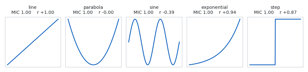
Five panels showing a line, a parabola, a sine wave, an exponential and a step function, each labeled with its MIC and its Pearson r

Fig. 1. MIC returns 1.00 on all five noiseless shapes while Pearson r ranges from +1.00 to -0.00

MIC returns 1.00 five times. Pearson returns +1.00 on the line, -0.00 on the parabola, -0.39 on the sine. The parabola is the case that matters: the relationship is exact, y a pure function of x, and correlation reports nothing. A script sorted by absolute r would discard that feature first.

That row of 1.00 is the easy half. All five relationships are deterministic, so any statistic obeying the definition must return its maximum on all five: the flat row is arithmetic. The hard half is whether the scores stay level under equal noise, which Fig. 6 measures, not assumes.

Now the catch, which governs everything after it. Two columns of independent random numbers, 200 points each, score about 0.22 on the same library, and the value moves with sample size, ties and marginals. A MIC of 0.22 on market data is indistinguishable from two unrelated columns, and becomes information only against what the same data scores with the relationship destroyed. That gap is what the rest of the article computes.

What MIC actually measures

The definition has two steps, the first the characteristic matrix. Lay a grid of i columns and j rows over the scatter plot, count the points per cell, and compute the mutual information of that table. Do it for every placement of the lines, keep the largest, and divide by the most an i by j grid could carry:

M[i][j] = max{ I(D,G) : G has i columns and j rows } / log2(min(i,j))

The second step is the maximum over grid shapes, capped:

MIC = max{ M[i][j] : i * j <= B(n) }, B(n) = n^0.6

Both parts carry weight. Dividing by log2(min(i,j)) stops a fine grid winning by default, since a finer grid always captures at least as much mutual information, and the cap on i times j stops a grid so fine every point owns a cell and scores 1.0 on noise. The exponent 0.6 is the paper's, exposed and clamped to [0, 1]: above 1 the budget exceeds n and everything scores near 1.0.

The search over grid shapes is the whole method. The same 220 points, a noisy sine, under two grids.

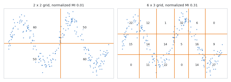
Two scatter plots of the same noisy sine wave, the left one cut by a 2 by 2 grid scoring 0.01, the right one cut by a 6 by 3 grid scoring 0.31, with the point count printed inside each cell

Fig. 2. A 2 by 2 grid sees nothing in a symmetric sine; a 6 by 3 grid over the same points scores 0.31

The coarse grid scores 0.01: a sine spends as much time above the midline on the left half as the right, so a two-column split sees two near identical distributions. The finer grid separates peaks from troughs and scores 0.31. The statistic is the maximum over both, hence the cap and the normalization.

One property removes work. MIC depends only on how points fall into bins, so any strictly monotonic transform of either axis moves the bin edges with the points. Scaling x by 1000, shifting y by 500, exponentiating x and swapping the arguments all return the identical double, error 0.000e+00, so no feature is standardized.

Computing it without trying every grid

The definition asks for a maximum over every placement of every grid, which is combinatorial and hopeless above about 20 points. MINE approximates it in three moves: cut one axis into bins of roughly equal population and freeze it, partition the other against it exactly, then swap the axes and keep the better of the two per cell.

Everything is measured in bits and computed from integer counts, which is what makes the library fast. Entropy is written as log2(n) minus a sum of k log2(k), not the familiar sum of p log p, because the first form takes integer arguments:

//+------------------------------------------------------------------+
//| Shannon entropy in bits of a distribution given as raw counts    |
//+------------------------------------------------------------------+
static double CMICEntropy::EntropyCounts(const int &counts[], const int len)
  {
   double total = 0.0;
   for(int i = 0; i < len; i++)
      if(counts[i] > 0)
         total += (double)counts[i];
   if(total <= 0.0)
      return(0.0);
 
   double acc = 0.0;
   for(int i = 0; i < len; i++)
      acc += XLogX((double)counts[i]);
   return(MathLog(total) / MIC_LN2 - acc / total);
  }

Since every argument is an integer bounded by the sample size, k log2(k) is tabulated once per data set and read back as an array index. The grid search evaluates entropies millions of times per coefficient, so CMICLogTable is the difference between a usable library and an unusable one.

Equipartition: the axis that is frozen

The frozen axis is cut into bins of roughly equal population. The subtlety is ties:

//+------------------------------------------------------------------+
//| Splits points into nbins groups of roughly equal population      |
//|                                                                  |
//|  Points sharing a value MUST land in the same group. Otherwise   |
//|  the split would depend on how the sort broke a tie, and the     |
//|  coefficient would stop being a function of the data. That       |
//|  constraint is also why fewer bins than requested can come back: |
//|  one repeated value can be more than a bin's worth of points on  |
//|  its own. Callers must read the return value, never assume it.   |
//+------------------------------------------------------------------+
static int CMICPartition::Equipartition(const double &vals[], const int n,
                                        const int nbins, int &binOf[])
  {
   ArrayResize(binOf, n);
   if(n <= 0 || nbins < 1)
      return(0);
 
   int idx[];
   CMICSort::IndexSort(vals, n, idx);
 
   int    curr    = 0;
   int    inRow   = 0;
   double desired = (double)n / (double)nbins;
 
   int i = 0;
   while(i < n)
     {
      int    j = i;
      double v = vals[idx[i]];
      while(j < n && vals[idx[j]] == v)
         j++;
      int size = j - i;
 
      double lhs = MathAbs((double)(inRow + size) - desired);
      double rhs = MathAbs((double)inRow - desired);
      if(inRow != 0 && lhs >= rhs)
        {
         curr++;
         inRow = 0;
         int left = nbins - curr;
         desired = (left > 0 ? (double)(n - i) / (double)left : (double)(n - i));
        }
 
      for(int t = i; t < j; t++)
         binOf[idx[t]] = curr;
      inRow += size;
      i = j;
     }
   return(curr + 1);
  }

Ties must stay in one bin, which is why the routine can return fewer bins than asked and the caller must read the return value. The two clock features are the extreme case: on the daily gold feed, hour of day is constant and day of week takes six values, so no equipartition of either returns more.

Clumps: why the optimization is tractable

The other axis is optimized exactly, and what makes that affordable is where a cut can usefully go. Sort by x: a run of consecutive points sharing one row never benefits from a cut through its middle, since splitting a pure column in two adds no information. The optimizer considers only the boundaries between such runs, which the library calls clumps, and a second pass caps their number.

The cap is a multiple of the column count, and the multiplier is measured. On one pass over the same 700 rows of gold, a factor of 2 gives MIC 0.069696 in 3.57 ms, 5 gives 0.136734 in 5.98 ms and 15 gives 0.148040 in 25.93 ms. The library ships 5: 2 is wrong by nearly a factor of two, and 15 buys 0.011 more for 4.3 times the time.

The dynamic program

With rows fixed and cuts reduced to clump boundaries, the best column partition is a shortest path problem. The paper's recurrence carries a rescaling term because it defines subproblems over normalized distributions; this one uses an additive form reaching the same optimum, which exhaustive search can verify because both maximize the same sum:

I(P;Q) = H(Q) + (1/n) * sum over columns of colScore

where colScore is the sum of xlogx of a column's per-row counts minus xlogx of its total. H(Q) is frozen and every column contributes independently, so the best partition into l columns is the best into l-1 plus one:

   // the contribution of a single column spanning clumps (a, b]
   int stride = m + 1;
   for(int a = 0; a < m; a++)
     {
      int baseA = a * q;
      for(int b = a + 1; b <= m; b++)
        {
         int    baseB = b * q;
         double s     = 0.0;
         int    tot   = 0;
         for(int r = 0; r < q; r++)
           {
            int cnt = m_prefix[baseB + r] - m_prefix[baseA + r];
            if(cnt > 0)
              {
               s   += m_log.Value(cnt);
               tot += cnt;
              }
           }
         m_score[a * stride + b] = s - m_log.Value(tot);
        }
     }
 
   int top = MathMin(maxCols, m);
   if(top < 2)
      return(true);
 
   // one column covering everything up to t
   m_prev[0] = MIC_UNSET;
   for(int t = 1; t <= m; t++)
      m_prev[t] = m_score[t];
 
   for(int l = 2; l <= top; l++)
     {
      for(int t = 0; t <= m; t++)
         m_curr[t] = MIC_UNSET;
 
      for(int t = l; t <= m; t++)
        {
         double bestv = MIC_UNSET;
         for(int s = l - 1; s < t; s++)
           {
            if(m_prev[s] == MIC_UNSET)
               continue;
            double v = m_prev[s] + m_score[s * stride + t];
            if(bestv == MIC_UNSET || v > bestv)
               bestv = v;
           }
         m_curr[t] = bestv;
        }
 
      if(m_curr[m] != MIC_UNSET)
         best[l] = m_lastHQ + m_curr[m] / (double)n;
 
      for(int t = 0; t <= m; t++)
         m_prev[t] = m_curr[t];
     }
   return(true);
  }

Entries no partition can reach are left at a sentinel, not at zero, and callers must test for it: an unreachable grid shape is not one that scored nothing.

The sweep

One direction of the search is a loop over row counts; the whole search is that loop run twice with the arguments swapped:

//+------------------------------------------------------------------+
//| One direction of the search                                      |
//|                                                                  |
//|  bVals is cut into j bins of equal population and then frozen;   |
//|  aVals is partitioned optimally against it. Called once each way |
//|  round, with transpose telling it which way the result should be |
//|  written into the matrix.                                        |
//+------------------------------------------------------------------+
void CMICMatrix::Sweep(const double &aVals[], const double &bVals[], const int n,
                       const bool transpose)
  {
   CMICSort::IndexSort(aVals, n, m_idx);
   for(int i = 0; i < n; i++)
     {
      m_aSorted[i] = aVals[m_idx[i]];
      m_bSorted[i] = bVals[m_idx[i]];
     }
 
   int stride  = m_b + 1;
   int maxRows = m_b / 2;
 
   for(int j = 2; j <= maxRows; j++)
     {
      int maxCols = m_b / j;
      if(maxCols < 2)
         continue;
 
      int q = CMICPartition::Equipartition(m_bSorted, n, j, m_rowOf);
      if(q < 2)
         continue;
 
      CMICPartition::Clumps(m_aSorted, m_rowOf, n, m_clumpRaw);
      int m = CMICPartition::Superclumps(m_clumpRaw, n, m_clumpFactor * maxCols,
                                         m_clumpOf);
      if(m < 2)
         continue;
 
      if(!m_opt.Solve(m_clumpOf, m_rowOf, n, m, q, maxCols, m_best))
         continue;
 
      int top = MathMin(maxCols, m);
      for(int l = 2; l <= top; l++)
        {
         double v = m_best[l];
         if(v == MIC_UNSET)
            continue;
         double norm = CMICEntropy::Log2((double)MathMin(l, q));
         if(norm <= 0.0)
            continue;
         double score = v / norm;
 
         int ci = (transpose ? j : l);
         int ri = (transpose ? l : j);
         if(ci > m_b || ri > m_b)
            continue;
 
         int at = ci * stride + ri;
         if(m_cell[at] == MIC_UNSET || score > m_cell[at])
            m_cell[at] = score;
         if(!transpose &&
            (m_fwdCell[at] == MIC_UNSET || score > m_fwdCell[at]))
            m_fwdCell[at] = score;
        }
     }
  }

Fixing y and optimizing x is a different approximation from the reverse, and neither dominates. Keeping the better per cell makes the result symmetric in its arguments, which the definition requires and the suite checks to the last bit.

Two details differ from the paper: the normalization uses log2(min(l, q)), the row count the equipartition achieved rather than the j it was asked for, and unreachable column counts stay unset where the paper pads them with I[k][l] = I[k][k]. Neither moves MIC or MCN, though MAS and MEV can shift on heavily tied columns.

The matrix that comes out has a distinctive shape, because the budget allows only i times j cells:

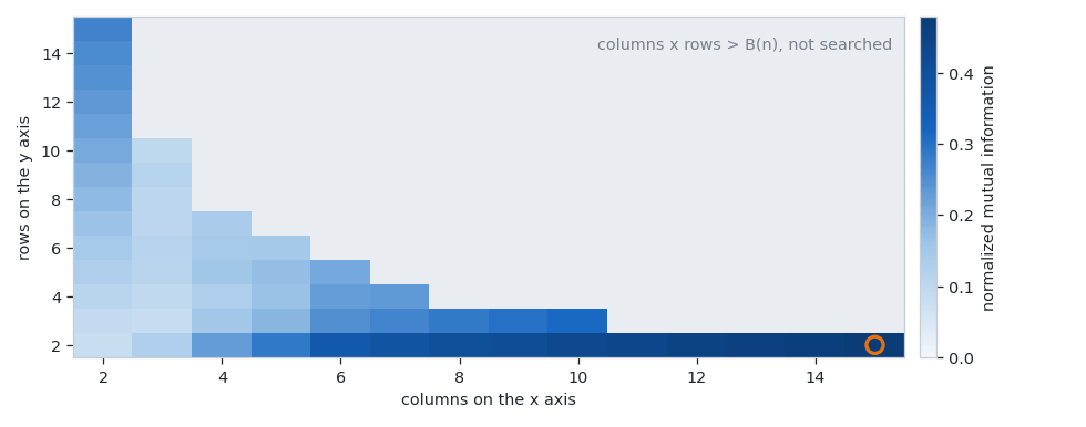
A heat map of normalized mutual information by grid shape, with a staircase boundary marking the grid budget and the winning cell circled at the bottom right

Fig. 3. The characteristic matrix for a noisy sine; the grey staircase is the budget and the circled cell is the maximum MIC reads off

Everything above the grey staircase is a grid the search may not try; MIC is the largest value below it.

Cost is measured with GetMicrosecondCount, never GetTickCount, whose 15-millisecond quantum is the same order as the thing being timed. One coefficient at 700 rows takes 5.97 ms, the fastest of three repeats, spreading to 6.01 ms. Twelve features at 100 permutations is 1212 coefficients, about 7.2 seconds, and the Python blueprint is two orders of magnitude slower.

The four MINE statistics

The search that produced MIC has already visited every grid, so three further statistics come out of it free. The result structure states what each is for:

//+------------------------------------------------------------------+
//| SMICResult                                                       |
//|                                                                  |
//|  One pair of variables, summarized.                              |
//|                                                                  |
//|  mic is the headline: how strong the dependence is, on a 0 to 1  |
//|  scale that does not care what shape the dependence has. That    |
//|  shape invariance is what lets two mic values be compared at a   |
//|  FIXED sample size. It does not make them comparable ACROSS      |
//|  samples: the level independent columns reach moves with n,      |
//|  with ties and with the marginals, so a mic from 200 rows and a  |
//|  mic from 700 rows sit on different floors and only a null       |
//|  places either of them.                                          |
//|                                                                  |
//|  mas, mev and mcn describe the KIND of dependence, and they come |
//|  free because the same search already visited every grid.        |
//|                                                                  |
//|  pearson is carried alongside so both readings can be seen at    |
//|  once: a high mic with a high r*r says nothing correlation did   |
//|  not already say, and a high mic with a low r*r is the case      |
//|  this statistic exists for. MicMinusR2() returns the gap between |
//|  them as a SCREENING contrast, not a decomposition - the two are |
//|  different estimators carrying different noise floors, so their  |
//|  difference does not partition the dependence into a linear and  |
//|  a nonlinear share and should not be read as a quantity.         |
//|                                                                  |
//|  bestCols and bestRows record the grid that produced mic, and    |
//|  fwdCols/fwdRows the best grid from the sweep that optimizes the |
//|  x axis specifically - that one can be turned back into cut      |
//|  points, so it is what a decision rule is built from.            |
//+------------------------------------------------------------------+
struct SMICResult
  {
   bool              valid;
   int               n;              // sample size
   int               b;              // B(n), the grid cell budget
   double            mic;            // maximal information coefficient
   double            mas;            // maximum asymmetry score
   double            mev;            // maximum edge value
   double            mcn;            // minimum cell number at eps = 0
   double            pearson;        // linear correlation, for contrast
   int               bestCols;
   int               bestRows;
   double            micFwd;         // best cell from the x-optimizing sweep
   int               fwdCols;
   int               fwdRows;
 
   double            MicMinusR2(void) const { return(mic - pearson * pearson); }
   double            R2(void) const { return(pearson * pearson); }
  };

MIC is the headline; the other three describe the kind of dependence, not its strength. MAS is the largest disagreement between a cell and its transpose, separating a non-monotonic shape from a monotonic one. MEV asks how much of the dependence a grid of two rows or two columns already captures. MCN is a complexity reading, log2 of the smallest grid still reaching the maximum.

Two qualifications come with that, and both matter later.

The first is how far MIC values can be compared. Shape invariance lets two coefficients be read against each other at one fixed sample size, which is all Fig. 1 shows; it is no license to compare across samples. The level unrelated columns reach moves with n, ties and marginals, so a MIC of 0.22 on 200 rows and one on 700 stand on different floors, and only a null places either.

The second is MCN. The paper defines it with a tolerance, log2 of the smallest grid scoring at least (1 - eps) times MIC. The mcn field above is the eps = 0 case, the grid actually chosen and what minepy reports by default; CMICMatrix::MCNAt takes any eps. Quoting one against a published MCN means matching the eps first.

A straight line and a sine wave with no noise both score MIC 1.000, while MAS reads 0.000 against 0.927 and MCN at eps = 0 reads 2.000 against 4.585. Equally strong, entirely different shapes.

Pearson's r rides alongside so both readings can be seen at once, and the library exposes the gap as MicMinusR2: 1.0000 on the parabola, 0.9833 on the sine, 0.0000 on the line. That gap is a screening contrast, not a decomposition: MIC and r squared are different estimators on different noise floors, so their difference splits the dependence into nothing and is not a quantity. Its job is sorting: a large gap says correlation would have missed this column.

Important: on noiseless data many grids reach exactly 1.0 by different routes, a unit or two in the last place apart: 15 tie on a line, 25 on a step. Taking whichever compared larger would hand the winning grid, and the bin count a rule is built with, to the rounding. Ties therefore resolve toward the coarsest grid.

The number that is not zero

Everything so far computes a coefficient. This section is why a coefficient alone is not a result. Run the library on pairs of independent Gaussian columns, where the answer is known, averaging over repeated draws at a range of sample sizes.

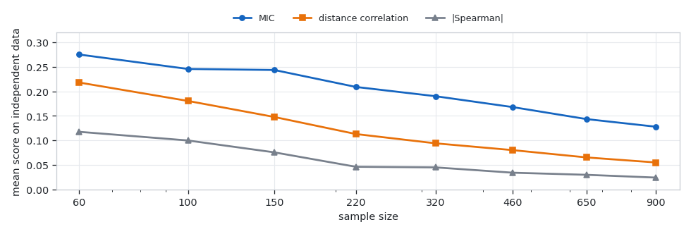
Three descending curves showing the mean score of MIC, distance correlation and absolute Spearman on independent random pairs as the sample size grows from 60 to 900

Fig. 4. None of the three reads zero on independent data, and the floor falls with sample size

MIC averages 0.275 at 60 points and 0.128 at 900. The floor is no constant: it moves with n, ties and marginals, so no threshold can be written once and applied everywhere. A rule acting on anything above 0.3 would fire constantly on small windows of noise and never on large ones.

The fix is the permutation null. Shuffle one column against the other, recompute, repeat. Shuffling keeps every value, tie and tail, so both marginals survive untouched and the null answers the right question: how high would this coefficient have gone if the two columns had nothing to do with each other?

On unordered data that is all a shuffle disturbs. On a time series it is not, and the scanning section returns to it: a forward return carries structure along its own index, and an ordinary shuffle destroys that too.

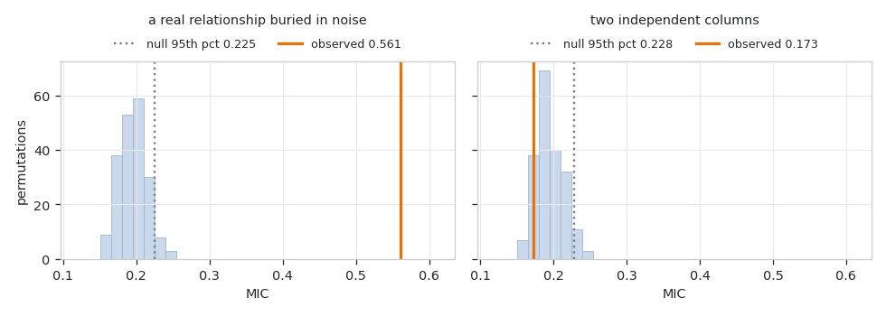
Two histograms of 200 permutation draws, the left with the observed MIC far to the right of the distribution, the right with the observed MIC inside it

Fig. 5. 200 permutation draws under two conditions: the observed 0.561 clears the null, the observed 0.173 sits inside it

Both nulls sit between roughly 0.15 and 0.25, the Fig. 4 floor measured on the data, not looked up. The observed 0.561 on the left is far outside it; the 0.173 on the right sits inside it, below its own 95th percentile of 0.228, which is correct because that panel is two independent columns.

The p-value uses the standard plus-one correction in both places, so it is never exactly zero. With k permutations the minimum possible p-value is 1/(k+1), and that single fact decides how many permutations are worth running.

At 15 permutations the floor is 0.0625 and nothing can ever be significant at 0.05. That failure is silent and looks like a market with no structure, so the library exposes RequiredPermutations and ResolutionNote and every consumer prints the note. At 20 the floor is 0.0476, which clears 0.05 and leaves one usable rung: every significant result arrives at that same number, so one that barely cleared its null is indistinguishable from one that cleared it by a mile. A p on the floor describes the resolution of the test, not the evidence.

So the scanner ships at 100 permutations, floor 0.0099, which is why the market section quotes p-values that are not all one number. The cost is linear: a second and a half at 20 becomes about seven at 100.

Twelve features and one winner

A single pair with a correct null is solved. A scan is not, and it flatters itself twice over.

The first is the search itself. Twelve features are tested and the largest kept, so each has a 5 percent chance of clearing its null by luck. Were they independent and each null correct, the chance one clears would be 1 - 0.95^12, about 46 percent. Neither holds: the features are strongly redundant, pushing the rate below 46, and the shuffle behind each null is wrong for an ordered target, pushing it far above. The measured rate is 95 percent, so that arithmetic is an order of magnitude, not a prediction.

The second is the shuffle. The target is a forward return over h bars, so two rows one bar apart share h-1 future bars and the column is autocorrelated by construction. Shuffling one value at a time destroys that autocorrelation with the pairing, giving a null built from a far choppier target, and too easy. Moving contiguous blocks keeps the runs intact:

//+------------------------------------------------------------------+
//| Fisher-Yates on contiguous BLOCKS rather than single values      |
//|                                                                  |
//|  A permutation null should destroy the pairing between the two   |
//|  columns and disturb as little else as it can. Shuffling one     |
//|  value at a time destroys much more: it also destroys the        |
//|  target's own autocorrelation, and a forward return over h bars  |
//|  is autocorrelated by construction, because neighboring rows     |
//|  share h-1 of the very same future bars.                         |
//|                                                                  |
//|  The result is a null that is too EASY - it compares a smooth    |
//|  feature against a target far choppier than the real one, which  |
//|  understates how often noise alone produces a high coefficient.  |
//|  Measured over 100 pure random walks in MIC_Test_Null: an iid    |
//|  shuffle let the search clear its own null on 95% of walks and   |
//|  the family-wise null on 46%, against a nominal 5%.              |
//|                                                                  |
//|  Moving blocks keeps the runs intact and breaks only the         |
//|  alignment between the columns, but it is not a clean null       |
//|  either, and the caller owns two caveats.                        |
//|                                                                  |
//|  First, a block shuffle PRESERVES the target's structure inside  |
//|  a block and SEVERS it at every boundary, so the permuted target |
//|  carries about n/block artificial joins and a little less        |
//|  autocorrelation than the real one. The bias that leaves is      |
//|  toward a null that is still slightly too easy, never too hard.  |
//|                                                                  |
//|  Second, the default of twice the horizon is measured, not       |
//|  derived. One horizon is already enough to separate rows that    |
//|  share no forward bars, so the extra factor buys margin rather   |
//|  than independence; the block sweep in MIC_Test_Null is the      |
//|  whole justification for the number, and it is a sweep precisely |
//|  because no argument picks it. A block length of 1 is exactly    |
//|  the plain shuffle again, kept so the two can be compared.       |
//+------------------------------------------------------------------+
void CMICRandom::ShuffleBlocks(double &arr[], const int n, const int block)
  {
   if(block <= 1 || n <= block)
     {
      Shuffle(arr, n);
      return;
     }
 
   int nb = (n + block - 1) / block;
   if(ArraySize(m_order) < nb)
      ArrayResize(m_order, nb);
   if(ArraySize(m_scratch) < n)
      ArrayResize(m_scratch, n);
 
   for(int i = 0; i < nb; i++)
      m_order[i] = i;
   for(int i = nb - 1; i > 0; i--)
     {
      int j = Below(i + 1);
      int t = m_order[i];
      m_order[i] = m_order[j];
      m_order[j] = t;
     }
 
   int at = 0;
   for(int b = 0; b < nb; b++)
     {
      int from = m_order[b] * block;
      int len  = MathMin(block, n - from);
      for(int k = 0; k < len; k++)
         m_scratch[at++] = arr[from + k];
     }
   for(int i = 0; i < at; i++)
      arr[i] = m_scratch[i];
  }

A blocked shuffle is better than an iid one and still not a clean null. It preserves structure inside each block and severs it at every join, so a permuted target of n rows in blocks of b carries about n/b artificial joins and slightly less autocorrelation than the real series. That bias points the same way, toward a null still too easy.

Nor is the default of twice the horizon derived. One horizon already separates rows sharing no forward bars, so the second factor buys margin, not independence. The sweep below is the only justification, and it is a sweep because no argument picks the number.

The generator is the library's own, because MathRand cannot do this job: 15 bits, far too short a period, and a global state two nulls would share. splitmix64 into xorshift64 star is unsigned 64-bit arithmetic, and MQL5's ulong wraps the way Python's masked integers do.

The correction never needs that 46 percent. Rather than split an error budget across a count of tries, it builds the null of the maximum: every permutation rescores all twelve against the same shuffled target and records the largest, the question actually asked when only the winner is kept. Because the twelve move together in every draw their redundancy is priced in, and no independence is assumed. It costs nothing extra:

      for(int p = 0; p < m_nperm; p++)
        {
         rng.ShuffleBlocks(perm, n, m_lastBlock);
         double mx = 0.0;
         for(int k = 0; k < m_count; k++)
           {
            for(int i = 0; i < n; i++)
               xf[i] = cols[k * n + i];
            double v = 0.0;
            if(m_engine.Compute(xf, perm, n, tmp))
               v = tmp.mic;
            draws[k * m_nperm + p] = v;
            if(v > mx)
               mx = v;
           }
         maxDraw[p] = mx;
        }
      m_micUs   += GetMicrosecondCount() - tn;
      m_micCalls += m_count * m_nperm;
 
      for(int k = 0; k < m_count; k++)
        {
         double real = m_score[k].stat.mic;
         m_score[k].hasNull = CMICNull::Summarize(draws, k * m_nperm, m_nperm,
                                                  real, m_score[k].nul);
         if(m_score[k].hasNull)
            m_score[k].significant = (m_score[k].nul.pValue <= m_maxP);
 
         int atLeast = 0;
         for(int p = 0; p < m_nperm; p++)
            if(maxDraw[p] >= real)
               atLeast++;
         m_score[k].pFamily = (double)(atLeast + 1) / (double)(m_nperm + 1);
         m_score[k].significantFamily = (m_score[k].pFamily <= m_maxP);
        }

One shuffle per permutation scored against every feature costs the same coefficients separate per-feature nulls would, and yields both those nulls and the distribution of the winner.

Whether either correction is sufficient alone is a question about a rate, and a rate needs runs behind it. The table is 100 pure random walks, twelve features, 100 permutations, horizon five, where the correct firing rate is the nominal 5 percent. Every cell carries a Wilson 95 percent interval, because two cells whose intervals overlap have not been told apart however different they look.

Shuffle block length	Per-feature gate fires	Family-wise gate fires
1 (plain shuffle)	95% (95/100), CI 88.8 to 97.8	46% (46/100), CI 36.6 to 55.7
5	60% (60/100), CI 50.2 to 69.1	17% (17/100), CI 10.9 to 25.5
10 (twice the horizon, the default)	51% (51/100), CI 41.3 to 60.6	9% (9/100), CI 4.8 to 16.2
20	40% (40/100), CI 30.9 to 49.8	6% (6/100), CI 2.8 to 12.5
40	45% (45/100), CI 35.6 to 54.8	5% (5/100), CI 2.2 to 11.2

Three readings, and the intervals decide all three.

The per-feature gate never works. Its best row is 40 percent, interval 30.9 to 49.8: blocking improves it enormously and still leaves it eight times nominal. A scan reporting the winner's own p-value is wrong on roughly half of all noise windows, whatever shuffle sits underneath.

The family-wise gate alone is not enough either. With a plain shuffle it fires on 46 percent of walks, interval 36.6 to 55.7, excluding 5 percent by a wide margin. A multiple-comparison correction cannot repair a null built wrong.

Together they land on nominal. At the default the family-wise gate fires 9 times in 100, interval 4.8 to 16.2, which covers 5 percent, and block 1's interval does not overlap block 10's, so the improvement exceeds sampling error.

What the table does not support is that twice the horizon is best. Blocks of 10, 20 and 40 give 9, 6 and 5 percent on intervals that overlap almost completely, so 100 walks cannot rank them. The defensible claim is narrower: the block must be at least the horizon, anything above that is consistent with nominal, and the default sits at the short end because a longer block severs more of the series.

MIC is not the only answer

MIC was challenged the moment it appeared, and presenting it alone is not presenting it honestly. Within weeks Simon and Tibshirani showed distance correlation detects real relationships more often at the same sample size, and Kinney and Atwal later showed in PNAS that MIC is not self-equitable. Neither retires the statistic; both make a MIC quoted with nothing beside it unreadable.

So the library carries the competition. Spearman is Pearson on the ranks and costs a sort, the cheapest check on whether a grid search was needed. Distance correlation is the real comparison: the population quantity is zero if and only if the two variables are independent, a guarantee neither rival offers, and it needs no bins, cap or tuning parameter.

That "if and only if" describes the population value and is the most misread sentence about this statistic. What the function below returns is a finite-sample estimate, biased upward, which does not read zero on independent data either: a cleaner statistic, not a free threshold.

//+------------------------------------------------------------------+
//| Distance correlation, Szekely, Rizzo and Bakirov 2007            |
//|                                                                  |
//|  Take every pairwise distance, double-center the matrix by       |
//|  subtracting its row mean, its column mean and adding back its   |
//|  grand mean, and correlate the two centered matrices entrywise:  |
//|                                                                  |
//|    A_ij   = |x_i - x_j| - rowMean_i - rowMean_j + grandMean      |
//|    dCov^2 = (1/n^2) SUM A_ij B_ij                                |
//|    dCor   = sqrt( dCov^2 / sqrt(dVarX^2 * dVarY^2) )             |
//|                                                                  |
//|  Two passes of n^2, and only O(n) memory - the row means come    |
//|  out of the first pass and the distances are cheap enough to     |
//|  recompute in the second. Holding the full n-by-n matrix would   |
//|  be 7.8 MB at the 700 rows this library scans, for no gain.      |
//|                                                                  |
//|  The distance matrix is symmetric, so a row mean and a column    |
//|  mean are the same number and one array serves for both.         |
//+------------------------------------------------------------------+
static double CMICContrast::DistanceCorr(const double &x[], const double &y[],
                                         const int n)
  {
   if(n < 3 || ArraySize(x) < n || ArraySize(y) < n)
      return(0.0);
 
   double arow[], brow[];
   ArrayResize(arow, n);
   ArrayResize(brow, n);
 
   double atot = 0.0, btot = 0.0;
   for(int i = 0; i < n; i++)
     {
      double sa = 0.0, sb = 0.0;
      for(int j = 0; j < n; j++)
        {
         sa += MathAbs(x[i] - x[j]);
         sb += MathAbs(y[i] - y[j]);
        }
      arow[i] = sa / (double)n;
      brow[i] = sb / (double)n;
      atot   += sa;
      btot   += sb;
     }
   double agrand = atot / ((double)n * (double)n);
   double bgrand = btot / ((double)n * (double)n);
 
   double sAB = 0.0, sAA = 0.0, sBB = 0.0;
   for(int i = 0; i < n; i++)
     {
      double ai = arow[i], bi = brow[i];
      for(int j = 0; j < n; j++)
        {
         double A = MathAbs(x[i] - x[j]) - ai - arow[j] + agrand;
         double B = MathAbs(y[i] - y[j]) - bi - brow[j] + bgrand;
         sAB += A * B;
         sAA += A * A;
         sBB += B * B;
        }
     }
 
   // a constant column double-centers to exactly zero, and no relationship
   // with a constant exists to report
   if(sAA <= 0.0 || sBB <= 0.0)
      return(0.0);
 
   // the 1/n^2 in front of all three sums cancels, and the two square roots
   // are taken separately so sAA*sBB is never formed - it overflows long
   // before either factor does
   double denom = MathSqrt(sAA) * MathSqrt(sBB);
   if(denom <= 0.0)
      return(0.0);
 
   double v = sAB / denom;                        // this is dCor SQUARED
   if(v <= 0.0)
      return(0.0);                                // rounding dust below zero
   if(v > 1.0)
      v = 1.0;                                    // Cauchy-Schwarz, defensively
   return(MathSqrt(v));
  }

The MQL5 side walks two passes of n squared and never forms the distance matrix, which would be 7.8 MB at the 700 rows this library scans; the Python reference double centers the matrices directly. The two must still agree, and the verification section reports by how much.

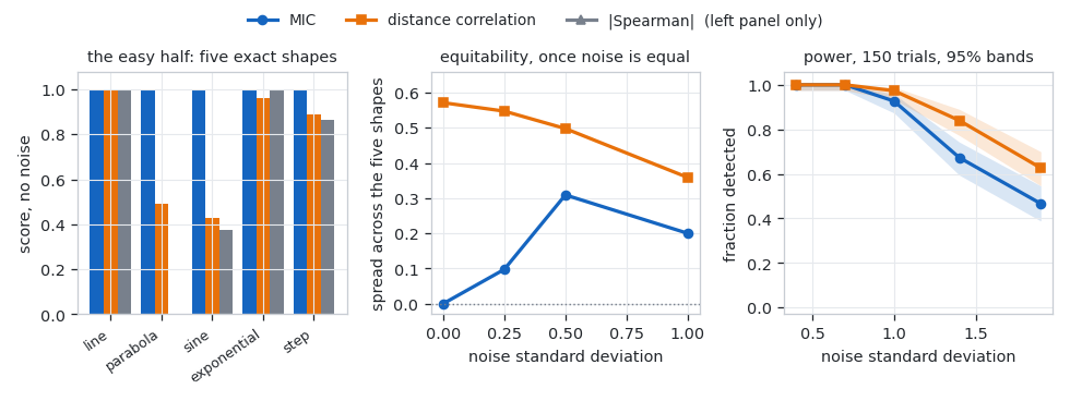
Three panels comparing MIC, distance correlation and absolute Spearman, showing scores on five noiseless shapes, the spread across those shapes under equal noise, and the detection rate for a buried sine as noise rises

Fig. 6. MIC is flat across five exact shapes, loses that flatness under equal noise, and has less power than distance correlation

The left panel is the claim as usually quoted: MIC's spread across the five noiseless shapes is 0.0000, distance correlation runs from 0.43 on the sine to 1.00 on the line, and Spearman collapses to zero on the parabola.

The middle panel is the claim tested. Each shape is standardized to unit variance, identical noise is added to all five, and the plot is the spread between the best and worst scoring shape over repeated draws. Perfect equitability would pin that at zero. It does not: MIC opens from 0.00 to 0.31 by a noise SD of 0.5, narrowing to 0.20 at 1.0 only because every shape is collapsing toward the floor together. That is Kinney and Atwal's result made visible, not cited. What survives is comparative: distance correlation's spread starts at 0.57 and never falls below 0.36, so MIC treats shapes far more alike than its rival, without treating them alike.

The right panel is power, and MIC loses it. The relationship is a sine buried in Gaussian noise at 100 points, detection means the real pair beat all its own shuffles, and each rate is 150 trials with a 95 percent band, since two rates separate only when their bands do. Below a noise SD of about 1 both find everything; above it the bands pull apart. The test script runs the same comparison harder: at a noise SD of 1.6, over 200 trials against 19 shuffles each, 100 detections for MIC against 137 for distance correlation, intervals 43.1 to 56.9 against 61.8 to 74.5. That is more than an ordering of two draws.

The noise floor goes the same way: on 200 points over 200 draws MIC averages 0.2210, distance correlation 0.1222, absolute Spearman 0.0596. The rival's floor is half MIC's and still nowhere near zero, so all three need a null. MIC needs it most.

Verifying a library with no reference to copy

The reference implementation of MINE is minepy, and it cannot be built here: it needs a C compiler and no wheel exists for the installed Python. Name that gap before the pass counts arrive. Nothing below shows this library agrees with the implementation the field uses. What it shows is consistency against oracles written independently of the code they test, and agreement with the published definition on samples small enough to enumerate.

The dynamic program against exhaustive enumeration, which is correct by construction because it tries everything. Worst of 534 partitions: 8.9e-16.
Mutual information two ways, H(rows) + H(cols) - H(joint) against a cell-by-cell p log(p / (px py)). Worst of 300 random tables: 3.9e-15, with the Python blueprint also checking against scikit-learn.
The whole matrix, not the maximum, since one number can agree by luck. 500 cells across 10 cases agree to 1.8e-15 in both directions, so neither side filled a cell the other left empty.
The null as an equality, not a comparison. Both languages run the same seeded generator and wrap 64-bit integers identically, so 240 draws across both shuffle styles reproduce at 0.000e+00.
The contrast statistics against numpy, the strongest rows because the implementations share nothing: distance correlation to 1.665e-13, Spearman to 1.110e-16.

One gap remains. Every check above compares the approximation to another implementation of the same approximation, never to the quantity being approximated. So the suite also computes exact MIC by enumerating every legal grid on both axes, affordable only on tiny samples, which is why MINE exists:

   double best = 0.0;
   for(int i = 2; i <= b; i++)
      for(int j = 2; j <= b; j++)
        {
         if(i * j > b)
            continue;
         if(i - 1 > nlx || j - 1 > nly)
            continue;                      // not enough distinct values
 
         double norm = CMICEntropy::Log2((double)MathMin(i, j));
         if(norm <= 0.0)
            continue;
 
         ArrayResize(table, i * j);
         ArrayResize(pickC, i - 1);
         ArrayResize(cutC, i - 1);
         for(int t = 0; t < i - 1; t++)
            pickC[t] = t;
 
         while(true)
           {
            for(int t = 0; t < i - 1; t++)
               cutC[t] = legX[pickC[t]];
            LabelFromCuts(rx, n, cutC, i - 1, colOf);
 
            ArrayResize(pickR, j - 1);
            ArrayResize(cutR, j - 1);
            for(int t = 0; t < j - 1; t++)
               pickR[t] = t;
 
            while(true)
              {
               for(int t = 0; t < j - 1; t++)
                  cutR[t] = legY[pickR[t]];
               LabelFromCuts(ry, n, cutR, j - 1, rowOf);
 
               ArrayInitialize(table, 0);
               for(int p = 0; p < n; p++)
                  table[colOf[p] * j + rowOf[p]]++;
 
               double v = CMICEntropy::MutualInfoTable(table, i, j) / norm;
               if(v > best)
                  best = v;
               gridsSeen++;
 
               if(!NextCombo(pickR, j - 1, nly))
                  break;
              }
 
            if(!NextCombo(pickC, i - 1, nlx))
               break;
           }
        }
   return(best);

The enumeration walks every grid shape the budget allows, then every legal set of column and row cuts, building the table and scoring it from the definition. Cuts splitting a run of equal values are excluded.

20 points, a budget of 9 cells and 2,342,776 grids enumerated across 40 cases produced two results. The approximation never scored above the true maximum, worst excess 0.000e+00, which it must, since MINE searches a strict subset of the grids. And it was exactly right on 28 of the 40 cases, median shortfall 0.0000, worst 0.2427.

That is easy to round in the flattering direction. A median of zero means the typical case is exact; a worst case of 0.2427 is a quarter of the scale, and on the other twelve the approximation is a lower bound, not MIC. The direction is guaranteed, the size is not.

Nor does it transfer. This is n = 20 at a budget of 9 cells, the only size where every grid can be enumerated; the scanner runs at n = 700 and a budget of 50. Nothing here says what the shortfall is there. The honest summary is narrow: on samples small enough to check, MINE matches the definition most of the time and never exceeds it.

Level	What it runs	Result
Blueprint	python mic_prototype.py	37 PASS, 0 FAIL
Entropy and RNG	MIC_Test_Entropy.mq5	25 PASS, 0 FAIL
Partition and DP	MIC_Test_Optimize.mq5	29 PASS, 0 FAIL
The coefficient	MIC_Test_Matrix.mq5	52 PASS, 0 FAIL
The null	MIC_Test_Null.mq5	34 PASS, 0 FAIL
Cross-check	export, then python mic_crosscheck.py	69 PASS, 0 FAIL

What gold actually says

The scanner builds twelve causal features from bars, scores each against a forward target, and repeats that on two controls built from the same data. Everything below is one run of MIC_Scan_Market.mq5 on XAUUSDm daily, Exness-MT5Trial15: 815 bars from 2024.02.19 to 2026.10.01 server time, 700 rows after warmup and horizon, horizon five, 100 permutations.

815 daily bars across that span is more than a five-session week gives, and the script prints why: Sunday 135, Monday to Thursday 137 each, Friday 132, six sessions a week over 136 weeks. This feed carries a short Sunday bar, which is why day of week takes six values. A reader checking the span against a calendar should expect six.

Both controls are rebuilt bars, not relabeled rows: the shuffle reorders the real log returns, re-cumulates them into a new price path, keeps the real bar times, and the features and target are recomputed from scratch. The control answers the same question as the real scan, not a neighboring one.

The twelve features raise a question of their own, and the all-pairs matrix answers it. This was the 2011 paper's headline application.

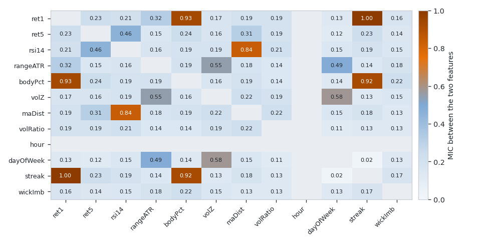
A twelve by twelve heat map of MIC between feature pairs, with several cells above 0.9 and the hour row greyed out as constant

Fig. 7. Every feature against every other on 700 rows of gold; pairs at or above 0.45 leave five clusters among the eleven live columns, and hour of day is constant here so it is not scored

Eight pairs sit at or above 0.45: the one-bar return and the direction streak share 0.995, the return and the body percentage 0.930, body percentage and streak 0.923, RSI and distance from a moving average 0.836. Grouping there leaves five clusters among the eleven live columns, so twelve names are nothing like twelve signals. The 0.45 line is a reading aid, not a test: nothing below roughly 0.2 is distinguishable from independence here, so the matrix is a map, not a set of claims.

That is a reason to drop columns. It is not a reason to call the correction below too harsh: a Bonferroni adjustment charged for twelve independent tries would be, but the family-wise null here is the maximum under one shared shuffle, which already moves correlated columns together in every draw.

The scan itself, counting features clearing the family-wise null at p of 0.05 or less. Eleven are counted, not twelve, because hour of day is constant on a daily chart: no grid can be laid on it, so it is reported unscanned, not as a measured zero.

Target	Real bars	Control: the same bars shuffled in time	Control: a matched Gaussian walk
Forward return	1 of 11 (volRatio, p = 0.0495)	0 of 11	0 of 11
Absolute forward return	0 of 11	1 of 11 (volRatio, p = 0.0297)	0 of 11
Forward volatility	2 of 11 (volRatio p = 0.0099, ret5 p = 0.0495)	1 of 11	0 of 11

Every control is scored against the same target as the scan it answers, because a finding about forward volatility can only be refuted by a control asked about forward volatility. One extra scan per target makes a row readable.

Read down the columns, not across a row. The direction target gives one survivor on real bars at p = 0.0495, a rung above the 0.0099 floor, and its controls give nothing. The absolute return target gives nothing on real bars and one survivor on the shuffled control at p = 0.0297, stronger than the only real hit above it. A lone survivor at the 0.05 gate is something these controls manufacture themselves.

Forward volatility is the only target where real bars pull ahead of their shuffle, two features to one, the strongest volRatio at MIC 0.2761 against a null 95th percentile of 0.2266, p = 0.0099. The family-wise correction keeps that honest: four of eleven cleared their own nulls and only two survive the maximum. At two to one it is a candidate worth more history, not a finding.

The scanner also walks the strongest feature through time, maDist against the absolute forward return, in 300-row windows every 50 rows, where three of nine clear. Those nine are not nine experiments: consecutive windows share five sixths of their data and the tracked feature is the winner of twelve judged against a null built for one. Neither effect is corrected, so three of nine shows how the reading moves, not a rate.

The practical follow up runs on the direction target, where a rule would be traded. MIC selects a feature and a bin count but no direction, so direction comes from the bins: read the mean forward return inside each and apply it to rows the fit never saw. The split is purged by the horizon.

Two things that table cannot undo are printed beside it, not assumed away. The four features are the in-sample top four, so every row is conditional on a selection it is not testing. And the decisions overlap: each is scored on a five-bar forward return, so neighbors share four bars, and a naive standard error is too small by roughly the square root of the horizon, the difference between a t of 2 and a t of 1. The SE column is Newey-West out to lag four.

Feature	In-sample mean	Out-of-sample mean	SE	Decisions	t	95% CI on the out-of-sample mean
volRatio	0.01926	-0.00431	0.00449	85	-0.96	-0.01311 to 0.00449
maDist	0.02136	-0.00534	0.00490	146	-1.09	-0.01495 to 0.00428
wickImb	0.02688	-0.00792	0.00408	115	-1.94	-0.01592 to 0.00008
streak	0.00869	-0.00413	0.00417	205	-0.99	-0.01230 to 0.00405

551 out-of-sample decisions, in-sample means positive on all four at two to five times the size, and every out-of-sample mean negative. The in-sample column alone would have read as four tradeable edges.

The interval column stops the negative column being over-read the other way. All four straddle zero, so none of the rules transferred and none reversed into something tradeable backwards. The nearest is wickImb at t = -1.94, the strongest of four rules picked out of twelve for being strongest in sample, exactly the selection no interval here corrects for.

Important: a negative result on one symbol and timeframe is a fact about that symbol and timeframe, not a proof about markets. What generalizes is the method: run the shuffled-bars control in the same pass and against the same target, and read the out-of-sample column as the answer.

The indicator

The indicator plots the rolling MIC of the strongest feature in a subwindow, explaining the absolute forward return by default, and with it the 95th percentile of the permutation null on the same window. That second line is not decoration: a coefficient of 0.22 means nothing alone, so only the gap carries information.

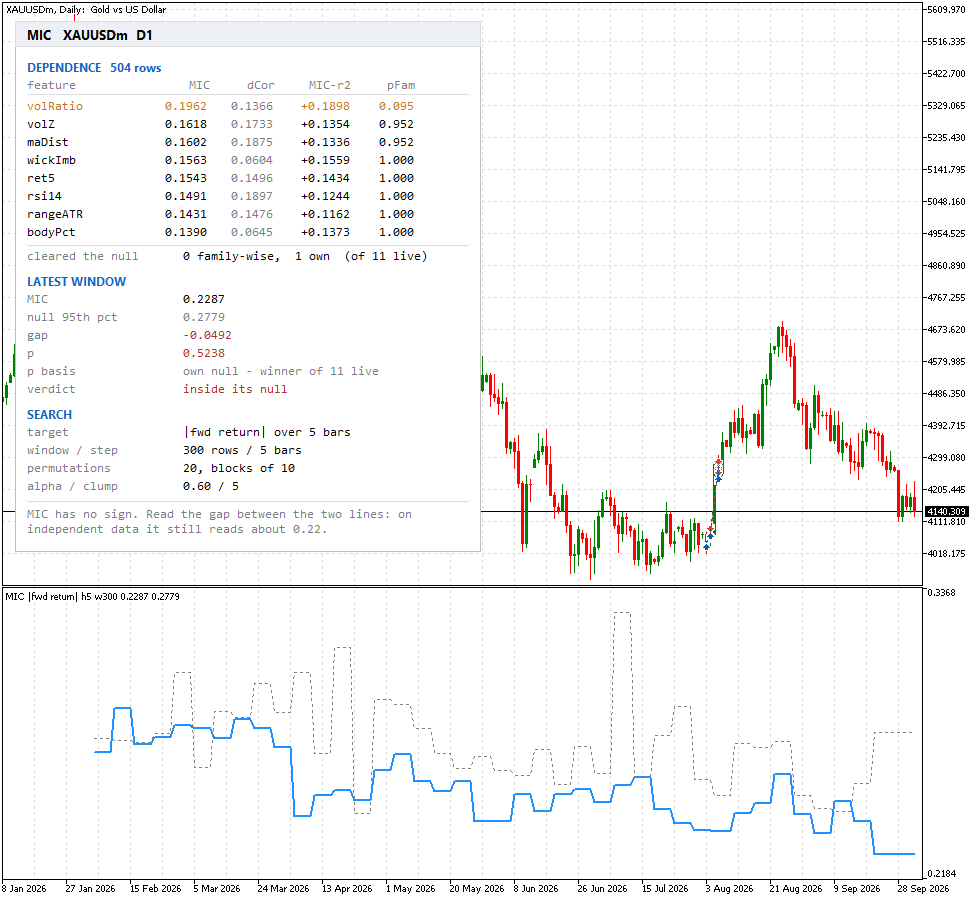
A MetaTrader 5 daily gold chart with the MIC indicator in a subwindow, showing the blue coefficient line running below the dotted null band for most of the window, and the ranked dependence panel on the chart to its left

Fig. 8. The indicator on gold daily: the solid line is the rolling coefficient, the dotted line its permutation null, and the panel ranks the strongest eight features

On gold daily with a 300-row window the coefficient ran from 0.2287 to 0.2879 while the null band ran from 0.2452 to 0.3265, and 5 of the 206 plotted bars sat above it. The same indicator on EURUSD H1 reads 0.1676 to 0.2525 against a band of 0.2035 to 0.2482, and clears on 56 of 206 bars.

Resist the obvious arithmetic. Five of 206 is not a 2.4 percent false positive rate, and 56 of 206 is not a 27 percent one, for two reasons.

First, 206 bars are not 206 readings. The line is a step: coefficient and null are recomputed every InpStep bars and held between, so at the shipped step of 5 the gold panel is 41 computed windows and the verification script counts 40 level changes. Counting bars inflates the denominator fivefold.

Second, even those 41 are not 41 experiments. Each window is 300 rows and the next starts 5 later, so consecutive windows share 295 of 300 rows, and across the whole span the display advances by under one window of fresh data. The plot holds roughly one independent reading. No percentage off this chart estimates a rate; the scan is where calibration is measured.

What the two symbols can be read for is the contrast. Eleven times as many flagged bars on EURUSD H1 as on gold daily is far too large to come from window overlap, so the H1 series genuinely spends more time above its band. A reason to look, not a result.

Cost sets the band's resolution. The indicator runs at 20 permutations rather than the scanner's 100 so the chart thread stays usable, and with 20 draws the 95th percentile is effectively the largest of them, so the dotted line is a noisy estimate of the ceiling. Raise InpPerms for the scanner's resolution and accept the time, measured inside the indicator with GetMicrosecondCount: the first load plotting 206 bars costs 2869 ms, about 13.9 ms a bar, repeated once per completed bar, never per tick.

The last trap is what the line tracks: the winner of the ranking table, chosen on the same bars it is drawn over, then judged against a null built for one feature. That is the multiple-comparison problem arriving through the choice of what to draw. Correcting it would cost twelve nulls a bar, so the indicator labels it and the table carries the family-wise p-value.

One property of the plot no test of the numbers can catch: a line of the correct length and shape drawn a few thousand bars too far to the left reads as an empty subwindow while every check of its values still passes. The buffers are therefore filled from the bar each row ENDS on, putting the reading under the bars it was computed from.

Conclusion

The Maximal Information Coefficient delivers a narrower version of what it promised. It scores a line, a parabola, a sine, an exponential and a step identically when they are equally noiseless, which no correlation coefficient does and is useful for screening, and it loses that flatness once they are equally noisy. What survives is comparative: MIC stays far flatter across shapes than distance correlation, and the gap to r squared sorts columns rather than measuring a nonlinear share.

The harder lesson is what the same tool says about a real market. Correcting the null took two fixes, a family-wise comparison and a blocked shuffle, and the measured rate says neither is sufficient alone. With both in place the direction target yields a single survivor while the shuffled control of a neighboring target yields one of its own at a smaller p-value, which says how little a lone survivor is worth. Forward volatility is the one target where real bars pull ahead of their shuffle, two features to one. All four strongest rules have out-of-sample intervals covering zero, so none transferred. That is a result, not a failure to find one.

What the article leaves you with:

A from-scratch MINE implementation: characteristic matrix, equipartition, clumps, dynamic program, and MIC, MAS, MEV and MCN.
A permutation null with a reproducible generator, block shuffling and a family-wise correction.
Distance correlation and Spearman alongside, so no coefficient is reported alone.
Four test scripts, a Python blueprint and a cross-check against exhaustive enumeration.
A scanner with two controls and a purged out-of-sample test with overlap-aware errors, and an indicator plotting the coefficient against its null band.

#	Filename	Type	Description
1	MIC.mqh	Include	Facade: scans every feature against the target, ranks them, builds the family-wise null and the all-pairs redundancy matrix
2	MICEntropy.mqh	Include	The x log x lookup table, Shannon entropy from counts, and mutual information of a contingency table
3	MICPartition.mqh	Include	Index sort, equipartition, clumps and superclumps
4	MICOptimize.mqh	Include	The dynamic program that finds the best axis partition for every column count in one pass
5	MICMatrix.mqh	Include	The characteristic matrix and the four MINE statistics, plus Pearson for contrast
6	MICContrast.mqh	Include	Spearman and distance correlation, the statistics MIC has to be judged against
7	MICRandom.mqh	Include	splitmix64 seeding into xorshift64 star, with plain and block shuffles
8	MICNull.mqh	Include	The permutation null and its summary statistics
9	MICData.mqh	Include	Bars into twelve causal features and one of three forward targets
10	MICRule.mqh	Include	The winning grid turned into equally populated bins, means and a direction
11	MIC_Test_Entropy.mq5	Script	Entropy against closed forms, mutual information two ways, and generator conformance
12	MIC_Test_Optimize.mq5	Script	The dynamic program against exhaustive enumeration, plus the partition rules
13	MIC_Test_Matrix.mq5	Script	Equitability, invariance, the noise floor, the approximation against exact MIC, and the rival statistics
14	MIC_Test_Null.mq5	Script	Reproducibility, the p-value floor, and the false positive rate of a twelve feature search on pure noise
15	MIC_Export_ForCrosscheck.mq5	Script	Exports 10 cases, the whole characteristic matrix, both nulls, the feature matrix and one rule for the Python cross-check
16	MIC_Scan_Market.mq5	Script	The market scan: three targets, the redundancy matrix, two controls, rolling windows, out-of-sample transfer and cost
17	MIC_Dependency_Scan.mq5	Indicator	Rolling MIC with its permutation null band and a ranked dependence panel
18	mic_prototype.py	Python	The blueprint the MQL5 library was written from, with its own oracles and self-test
19	mic_crosscheck.py	Python	Compares the MQL5 export against an independent Python recomputation
20	MQL5.zip	Archive	Archive with all project files in their subfolders; unpack it into the terminal data directory and every file lands in its required location

Attached files |

Download ZIP

MQL5.zip (105.35 KB)

Warning: All rights to these materials are reserved by MetaQuotes Ltd. Copying or reprinting of these materials in whole or in part is prohibited.

This article was written by a user of the site and reflects their personal views. MetaQuotes Ltd is not responsible for the accuracy of the information presented, nor for any consequences resulting from the use of the solutions, strategies or recommendations described.