Self-Exciting Markets: Building a Hawkes Process from Scratch

Contents

• Introduction
• What the library delivers
• A self-exciting process in one picture
• From price to an event train
• The exponential kernel: O(N) intensity and a closed-form integral
• The log-likelihood
• Fitting by maximum likelihood
• Trusting the numbers: verification without a reference package
• What it reads on real data
• An indicator and a demonstration EA
• Conclusion

Introduction

Every trader has seen it. A market drifts sideways for days, then a single sharp move breaks the calm, and suddenly the moves come one after another. The tape gets loud, then stays loud, then slowly settles. This is volatility clustering, and it is one of the most robust facts about financial time series.

The usual MQL5 answer to clustering is a GARCH-style volatility model. GARCH describes the size of returns and how their variance persists. It is a good tool, but it answers a different question from the one this article asks. GARCH models the amplitude of a continuous process. A Hawkes process models the timing of events: it treats large moves as discrete arrivals in time and asks whether one arrival raises the probability of the next.

That shift of viewpoint buys a single, interpretable quantity. The Hawkes branching ratio, written n, is the expected number of follow-on events each event triggers. When n is near zero the events are independent, arriving like raindrops with no memory. When n approaches one the process is close to feeding on itself, each move breeding more moves, a market that is endogenously driven rather than reacting to outside news. Economists call this property reflexivity, and n measures it on a scale from zero to one.

A search of the MQL5 article catalog turns up GARCH and its relatives, but no Hawkes process. So this is built from scratch: an event extractor, an exponential-kernel intensity, a maximum-likelihood fitter, and the branching ratio on top. The code is the deliverable, and it is tested to the point where its numbers can be trusted; this validation was done before a single line of the article was written.

One warning up front: it shapes everything that follows. A Hawkes process is a descriptive instrument, not a crystal ball. It tells you how clustered the recent past has been. On a calm, efficient market it will honestly read close to zero, and reading that zero as a fault is the most common way to misuse the tool.

What the library delivers

The whole library is a short pipeline. Price goes in, an event train comes out, the event train is fitted by maximum likelihood, and the fit yields the branching ratio and a conditional intensity you can plot. The diagram below is the entire program at a glance.

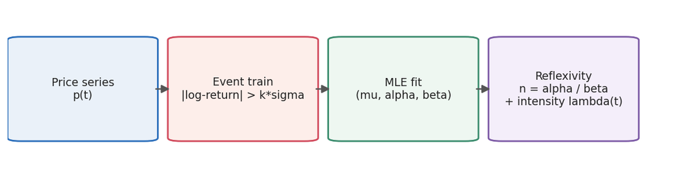
Fig. 1. The whole library as one pipeline: a price series becomes an event train, the train is fitted by maximum likelihood, and the fit returns the branching ratio n and a conditional intensity to plot

Reading right to left tells you what the caller receives. The fit returns the three model parameters, the branching ratio n, and enough state to evaluate the intensity at any time. An indicator turns that into a live panel and a plotted intensity curve. The verification is not a promise; it is a documented set of runs, stated in the section on trust. The kernel test reports 26 checks, the likelihood test 21, the fitter test 109, and an independent Python cross-check 51, using numbers exported from compiled MQL5.

That is what this article delivers. The rest explains how, starting with the process itself.

A self-exciting process in one picture

A point process is just a list of times at which something happens. What makes a process Hawkes is the way the rate of new events depends on the past. The conditional intensity, the instantaneous rate of events at time t, given everything that came before, is

lambda(t) = mu + sum over t_i < t of alpha * exp(-beta * (t - t_i))

Three parameters carry the model. The baseline mu is the background rate, the rate the process would run at with no self-excitation. Each past event t_i adds a jump of size alpha to the intensity, and that jump decays away at rate beta. So an event makes the next event more likely for a while, and the effect fades. The figure below shows exactly this: a synthetic price with its large moves marked, and underneath, the intensity that those moves drive.

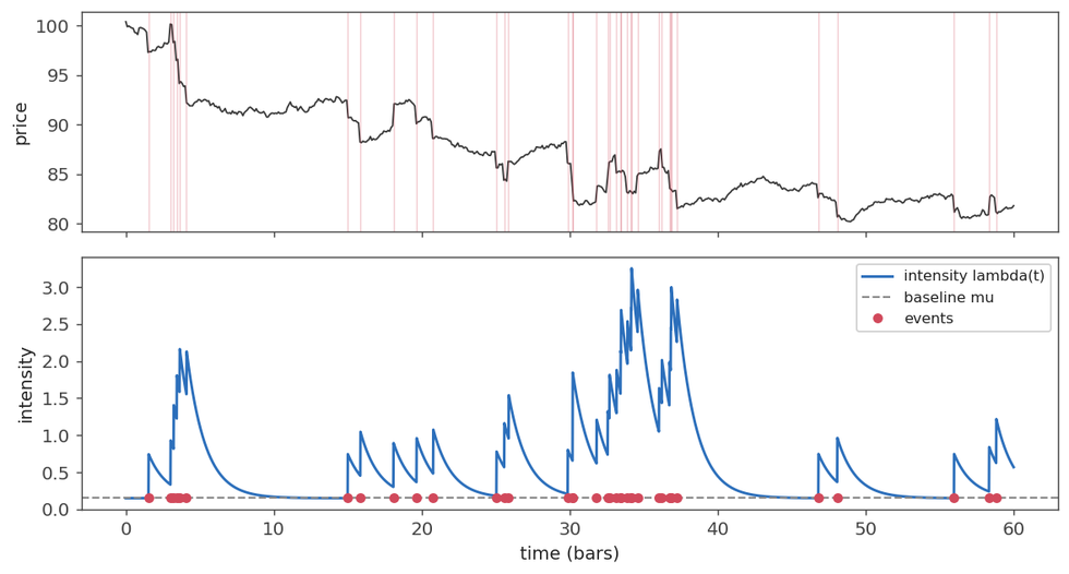
Fig. 2. A synthetic price with its large moves marked (top) and the conditional intensity those moves drive (bottom); the intensity leaps at each event and relaxes back toward the dashed baseline, and events that fall close together build into a tall hump

Notice how the intensity leaps the instant an event lands, then relaxes back toward the dashed baseline. When events fall close together the intensity never gets time to relax, so it builds into a tall hump. That hump is a cluster, drawn directly from the mathematics.

The single number that governs how tall the humps get is the ratio of the jump size to the decay rate. This is the branching ratio:

n = alpha / beta

It is the area under one event's contribution, and it equals the expected number of direct offspring each event produces. The process is stationary, meaning it does not explode, exactly when n is below one. The next figure holds the baseline fixed and raises n from 0.1 to 0.9. The event ticks at the bottom of each panel go from scattered to clumped, and the intensity above them goes from nearly flat to strongly peaked.

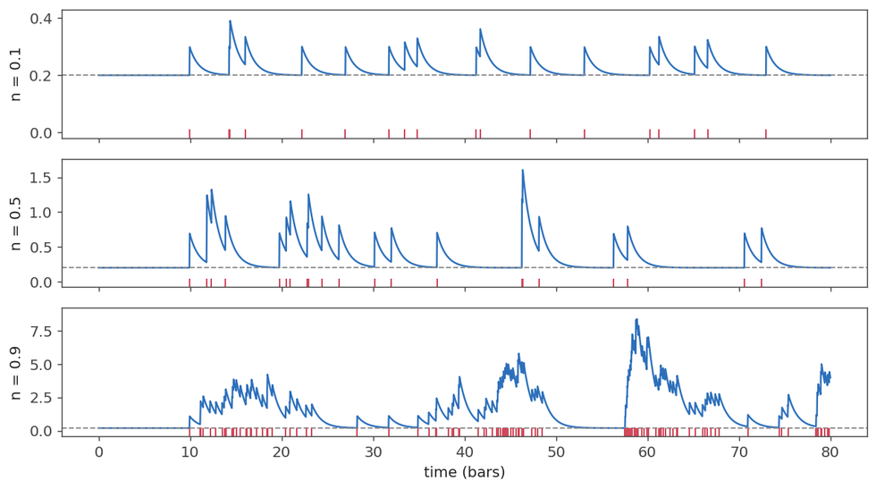
Fig. 3. The same baseline held fixed at branching ratios 0.1, 0.5, and 0.9; as n grows the events at the bottom of each panel go from scattered to clumped and the intensity above them from nearly flat to strongly peaked

This is the quantity the whole library exists to estimate. Everything else is machinery for turning a price chart into an event train and then recovering mu, alpha, and beta from it.

From price to an event train

The Hawkes model is not fitted to prices. It is fitted to a list of event times. So the first class, CHawkesData, has one job: turn a slice of the price series into that list. An event is defined as a bar whose absolute log-return exceeds k times the local standard deviation of returns. That is the standard "large move" definition, and it adapts to the market's current volatility rather than using a fixed threshold.

Two design choices in this class are load-bearing, and both were settled by measurement rather than taste. The first is the clock. Event times are measured inbars, not wall-clock seconds. On a seconds-based clock a daily bar gap is about 86400, the decay rate beta comes out near 1e-5, and the exponential recursion at the heart of the library loses all its precision to that scale. In bar units every inter-event gap is a small integer, and mu, alpha, and beta are all of order one. The choice of clock buys good conditioning, and it changes no answer because the model is defined on whatever clock you give it.

Here is the core of the extraction, the loop that walks the returns and pushes an event whenever one clears the threshold.

//+------------------------------------------------------------------+
//| Turn a slice of the price series into an event train             |
//+------------------------------------------------------------------+
//--- first return index with w returns strictly before it: ret[i-w .. i-1]
   int i0 = m_volWin + 1;
   m_origin = i0;

   for(int i = i0; i < count; i++)
     {
      //--- population std of the trailing window ret[i-w .. i-1]
      double s = 0.0, s2 = 0.0;
      for(int j = i - m_volWin; j < i; j++)
        {
         s  += ret[j];
         s2 += ret[j] * ret[j];
        }
      double mean = s / m_volWin;
      double var  = s2 / m_volWin - mean * mean;
      if(var < 0.0)
         var = 0.0;
      double sig = MathSqrt(var);

      if(sig > 0.0 && MathAbs(ret[i]) > m_k * sig)
        {
         double t    = (double)(i - i0);
         double mark = (ret[i] >= 0.0 ? 1.0 : -1.0);
         Push(t, mark, i);
        }
     }

The volatility is estimated from the window of returns strictly before the current bar, never including it. That causality matters: a jump must not be allowed to inflate the very yardstick it is measured against. The clock origin is set to the first bar that has a full trailing window behind it, so event times start at zero and the horizon is the number of bars actually watched.

The second choice is the trailing-window length. It is the subtlest part of the library. The obvious value is short, around 20 bars, to keep the volatility estimate local. That obvious value is wrong, and it took a direct experiment to see why. The threshold adapts to recent volatility, so a short window co-moves with the very clustering the model is trying to detect. A burst of large moves lifts its own trailing standard deviation, the follow-on moves then fail to clear k times that inflated sigma, and the cluster is normalized away before it ever reaches the event train.

To measure the effect, we built a synthetic price series with genuinely clustered jumps at Hawkes event times (true branching ratio 0.5). We then re-extracted events using different window lengths and refit the model. The result is the figure below.

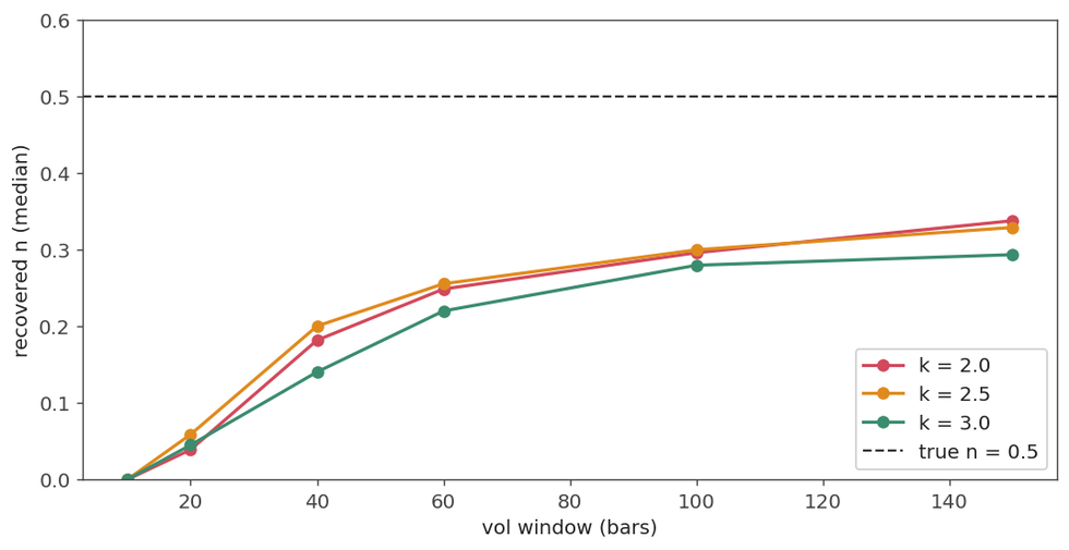
Fig. 4. Recovered branching ratio against vol-window length for a series with a true n of 0.5; a 20-bar window reads near zero because it normalizes the cluster away, while a 100-bar window recovers about 0.3, biased low but alive

At a 20-bar window the recovered branching ratio collapses to roughly 0.05, so the true clustering of 0.5 is read as pure noise. At 100 bars the estimate climbs back to about 0.3. The recovery is still biased low, because a slow window cannot undo all of the self-normalization, but the signal survives. For this reason the default window in CHawkesData is 100 bars, not 20. This is not a smoothing preference, it is a measured correction, and it means the branching ratio should be read as ordinal, more clustering versus less, rather than as a calibrated fraction.

Important: do not shorten the vol window back to about 20 bars for clustering work. A short window makes the threshold chase the cluster it is meant to detect, and the branching ratio reads far too low as a result.

The exponential kernel: O(N) intensity and a closed-form integral

The exponential kernel is not chosen for realism, it is chosen because it makes the arithmetic collapse. Two things that would otherwise cost O(N^2) become O(N), and both are needed on every single likelihood evaluation, so the saving is the difference between a usable fitter and an unusable one.

The first is the intensity just before each event. Writing A(i) for the sum of decayed contributions of all earlier events at the time of event i, the intensity there is mu + alpha * A(i). Computed directly, each A(i) is a sum over all earlier events, and the whole set is a double sum. But the exponential is memoryless, so A(i) can be built from A(i-1) with a single multiply and add. That recurrence is the spine of the library.

//+------------------------------------------------------------------+
//| A(i) via the memoryless recursion                                |
//+------------------------------------------------------------------+
bool CHawkesKernel::DecayFactors(const double &times[], int n, double beta,
                                 double &A[])
  {
   if(n < 0 || beta <= 0.0)
      return false;
   ArrayResize(A, n);
   double a = 0.0;
   for(int i = 0; i < n; i++)
     {
      if(i == 0)
         a = 0.0;
      else
         a = MathExp(-beta * (times[i] - times[i - 1])) * (1.0 + a);
      A[i] = a;
     }
   return true;
  }

The single line inside the loop, a = exp(-beta * gap) * (1 + a), is the whole idea. Decay the running sum forward to the current event, add one for the event that just landed, and carry it. There is a matching brute-force double sum in the same header, and it exists for one reason: the tests demand the recursion equal it to rounding.

The second saving is the integral of the intensity over the observation window, called the compensator. The likelihood needs it, and for a general kernel it would be numerical quadrature. For the exponential kernel it is a closed form:

integral from 0 to T of lambda(s) ds = mu * T + (alpha / beta) * sum over i of (1 - exp(-beta * (T - t_i)))

//+------------------------------------------------------------------+
//| Compensator Integral_0^T lambda(s) ds                            |
//+------------------------------------------------------------------+
double CHawkesKernel::Compensator(const double &times[], int n, double T,
                                  double mu, double alpha, double beta)
  {
   if(beta <= 0.0)
      return mu * T;
   double s = 0.0;
   for(int i = 0; i < n; i++)
     {
      if(times[i] > T)
         break;
      s += 1.0 - MathExp(-beta * (T - times[i]));
     }
   return mu * T + (alpha / beta) * s;
  }

Both pieces are one pass over the events. That is what keeps a full fit, which is thousands of likelihood evaluations, down to a few milliseconds on a normal window.

The log-likelihood

With the two pieces in hand the log-likelihood of a point process on the interval from 0 to T is short to state. It rewards putting intensity where events actually landed, and charges for carrying intensity everywhere else:

log L = sum over i of log(lambda(t_i)) - integral from 0 to T of lambda(s) ds

The implementation folds the event sum into its own pass rather than calling the intensity routine, so it can reject the instant any intensity turns non-positive, and it borrows the closed-form compensator for the second term.

//+------------------------------------------------------------------+
//| log L through one forward pass                                   |
//+------------------------------------------------------------------+
double CHawkesLikelihood::LogLik(const double &times[], int n, double T,
                                 double mu, double alpha, double beta)
  {
   if(beta <= 0.0 || mu < 0.0 || alpha < 0.0)
      return -DBL_MAX;

//--- event sum: sum_i log(mu + alpha * A(i)), A(i) recursive
   double sumLog = 0.0;
   double A = 0.0;
   for(int i = 0; i < n; i++)
     {
      if(i > 0)
         A = MathExp(-beta * (times[i] - times[i - 1])) * (1.0 + A);
      double lam = mu + alpha * A;
      if(lam <= 0.0)
         return -DBL_MAX;
      sumLog += MathLog(lam);
     }

//--- compensator: mu*T + (alpha/beta) sum_i (1 - exp(-beta (T - t_i)))
   double comp = CHawkesKernel::Compensator(times, n, T, mu, alpha, beta);

   return sumLog - comp;
  }

Returning the most negative possible value for an inadmissible parameter set, rather than throwing, lets the optimizer treat the whole box as one continuous surface and simply walk away from the bad corners. That keeps the search code free of special cases.

Fitting by maximum likelihood

Fitting means finding the mu, alpha, and beta that maximize log L. The search is deterministic on purpose: a fixed grid of starting points followed by a Nelder-Mead polish, with no random restarts, so the same event train gives the same answer on every machine. The one design decision worth dwelling on is the choice of search coordinates.

The natural parameters are mu, alpha, and beta, but the constraint that keeps the process stationary, alpha below beta, is an awkward diagonal wedge in that space. So the search runs over mu, the branching ratio n, and beta instead, recovering alpha as n times beta afterward. In these coordinates stationarity is the single flat wall n below one, and the box simply tops out just short of it, at 0.99. A non-stationary optimum is refused by the shape of the box, not by a fragile post-check. The mapping from the normalized cube back to the model takes three lines.

//+------------------------------------------------------------------+
//| Map normalised [0,1]^3 back to (mu, n, beta)                     |
//+------------------------------------------------------------------+
void CHawkesFitter::ToParams(const double &u[],
                             double &mu, double &nbr, double &beta) const
  {
   mu   = m_muLo   + u[0] * (m_muHi   - m_muLo);
   nbr  = m_nMin   + u[1] * (m_nMax   - m_nMin);
   beta = m_betaMin + u[2] * (m_betaMax - m_betaMin);
  }

The n and beta boxes are fixed, because in the bar clock both are order-one numbers on any timeframe. The mu box is resolved from the data: for a stationary process the expected intensity equals the empirical event rate, so mu is bracketed around that rate with a little headroom.

There is a trap here that the LPPL literature is famous for, and the fitter guards against it explicitly. A search bound and a qualification threshold must never be the same number, or a fit that wanted to go past the wall comes back resting exactly on it and gets waved through. When the polished result lands against a wall of the box, the fit records it. The distinction that matters most is n against the top wall, because that is a wanted-but-refused non-stationary fit, and its reported reflexivity is not an estimate at all.

//+------------------------------------------------------------------+
//| Grid scan, then Nelder-Mead from the best few grid points        |
//+------------------------------------------------------------------+
   //--- did the search stop against a wall? asked in u-space, no scaling.
   //--- nAtUpperBound is singled out because only the top wall discredits
   //--- the reflexivity reading (see the SHawkesFit note).
   out.muAtBound     = (winnerU[0] <= m_tolX || winnerU[0] >= 1.0 - m_tolX);
   out.nAtBound      = (winnerU[1] <= m_tolX || winnerU[1] >= 1.0 - m_tolX);
   out.nAtUpperBound = (winnerU[1] >= 1.0 - m_tolX);
   out.betaAtBound   = (winnerU[2] <= m_tolX || winnerU[2] >= 1.0 - m_tolX);

This distinction is not academic. It is exactly what separates a genuine low reading from a broken one, and the section on real data shows why lumping the two together led to a wrong conclusion on the first market scan.

Trusting the numbers: verification without a reference package

The honest problem with verifying a fitter is that you need something to check it against. For Matrix Profile there is a deterministic Python reference. For Hawkes there is not: the common Python packages either are not available on the current interpreter or seed their own optimizers randomly, so there is no fixed answer to demand. The library therefore verifies itself from the mathematics, in three independent ways.

The first is the intensity and the compensator. Both have closed forms, so an independent check is a brute-force O(N^2) double sum for the intensity and a midpoint Riemann sum for the integral, written straight from the definitions in Python. These give two comparisons that check different things. An independent Python re-implementation of the same O(N) recursion matches the compiled library to about 4.5e-12, which is bit-level: it confirms both languages run the identical arithmetic. The stronger check is the brute O(N^2) sum with the Riemann integral, which owes the recursion nothing and matches the library to about 2.8e-5. That gap is the quadrature floor of the reference integral, not an error in the library.

The second is the fitter, checked by parameter recovery. Event trains are simulated with known parameters using Ogata's thinning algorithm, then fitted, and the recovered branching ratio is compared to the planted one. Because the trains are random, the test asserts an invariant that noise cannot cross rather than a fragile point tolerance: the fitted log-likelihood must be at least as high as the log-likelihood at the true parameters, which the maximum-likelihood estimate must satisfy whenever the truth lies inside the box. On top of that it checks the median absolute error in n across a batch, which is far more stable than any single fit. The figure below shows the recovery across four regimes.

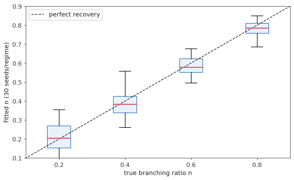
Fig. 5. Fitter recovery of the branching ratio across four regimes; the fitted values straddle the true 0.2, 0.4, 0.6, and 0.8, with the small downward bias that is the known finite-sample behavior of the estimator

The median absolute error in n sits around 0.04 to 0.05 across the regimes, with a small downward bias that is the known finite-sample behavior of the estimator. A genuinely Poisson process, with no self-excitation at all, reads a median n of 0.058, which is the honest zero of this estimator on samples of this size. The other two parameters, mu and beta, are deliberately left unchecked by tolerance: mu is barely identified when n is high, and beta is a nuisance direction. The branching ratio is the quantity the model is good at, and the only one worth asserting.

The third check ties the two languages together. The MQL5 program exports its event trains, its probe log-likelihoods, and its fitted parameters to file, and a Python script recomputes everything independently and compares. The full run reports 51 checks passing, with the fitted branching ratio matching to four decimals. Inside MQL5 the three test scripts report 26, 21, and 109 checks passing, in the kernel, likelihood, and fitter tests respectively. None of this proves the model is right for any market. It proves the code computes the model it claims to, which is the only thing code can be made to prove.

What it reads on real data

A market scan sweeps a real chart in sliding windows, fits each one, and reports the distribution of the branching ratio along with the diagnostics. The first honest lesson came from the diagnostics, not the profit. On an early gold H1 scan more than half the windows landed against a box wall, and the scan first reported this as degenerate and told the reader to ignore those readings. That was wrong, and the fitter's own bound flags are what corrected it.

The resolution is the distinction drawn in the fitting section. A process with no self-excitation drives alpha toward zero, which leaves the decay rate beta unidentified, so beta slides to a wall while n correctly rests on its lower wall near zero. That is not a degenerate fit, it is the exact signature of "no clustering here". Only an upper-bound hit on n (a refused non-stationary fit) discredits the estimate. This case was rare. Once the scan built its distribution from the reliable windows only, and reported upper-wall pins separately, the reading became sensible: gold H1 at these thresholds is close to Poisson, with a minority of windows showing real clustering. That is a legitimate result, and it is the expected contrast with a bubble detector, which reads zero almost everywhere because its target is rare. Clustering is common, so Hawkes reads a small positive number often, and a large one sometimes.

The scan is also where the vol-window correction from the extraction section earns its place. Before that fix, the low readings on gold were partly the short window hiding the clustering, not the market lacking it. The measured collapse in the earlier figure is why the default window is now long, and why the branching ratio should be read as ordinal.

An indicator and a demonstration EA

The indicator, Hawkes_Intensity, fits the trailing window once per new bar. It draws (1) the conditional-intensity line in a subwindow with event markers and the baseline, and (2) a compact main-chart panel with n, the verdict, the fitted parameters, and the current intensity. It costs a single fit per bar, a few milliseconds, so it does not stall the chart on load. The chart below shows the indicator running live, with the intensity line and events in the subwindow and the reflexivity panel on the main chart.

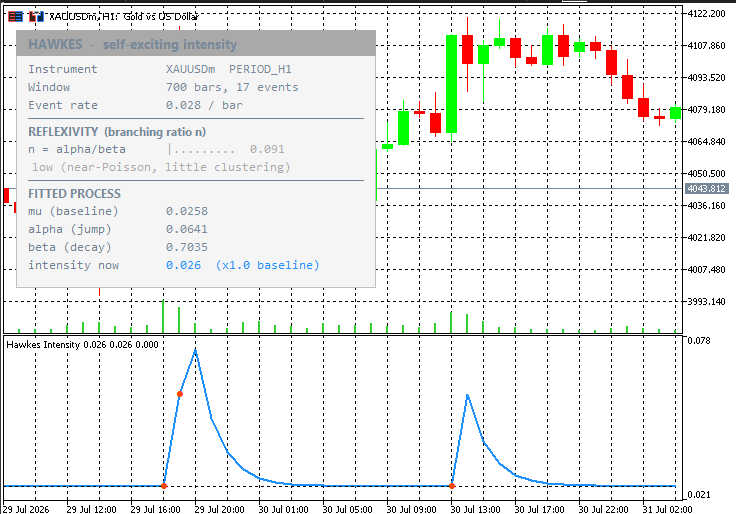
Fig. 6. The Hawkes intensity indicator on a live chart: the fitted intensity line and event markers in the subwindow, with the reflexivity panel carrying the branching ratio, the verdict, the fitted parameters, and the intensity now on the main chart

The panel is drawn with chart objects, a background rectangle and a stack of text labels, rather than with a comment, so the columns line up and the layout is stable. The intensity line does exactly what the earlier concept figure showed: it jumps at every event dot and decays back toward the baseline, so a cluster of dots holds the line high and a quiet stretch lets it fall.

The Expert Advisor, Hawkes_Reflexivity_EA, is a demonstration and nothing more. Its purpose is to show how the reflexivity reading is consumed by a trading rule, not to present an edge. It gates entries on three conditions at once: the branching ratio must be reliable and above a floor, so the regime genuinely self-excites; the intensity now must sit in the top of its own recent range, so a burst is currently active; and the most recent event must be fresh, which gives the direction. When all three hold, it follows the burst with one position and a time-based exit. The reflexivity gate is what makes it a Hawkes EA rather than a plain volatility filter: it refuses the near-Poisson regimes where clustering is not real.

Important: this EA is a teaching demonstration, not a trading system. No profit is claimed or implied. An exploratory run on XAUUSD H1 over a six-month window produced a few dozen trades and a positive return, but with an equity drawdown near 37 percent, no stop loss, and only a single in-sample period. Read it as an illustration of the gate firing, not as evidence of an edge. Any real use needs a stop, out-of-sample testing, and far more trades before a single number from it means anything.

The balance graph below is from a Strategy Tester run of the demonstration EA, so the gate's activations can be observed on a chosen symbol and period rather than described in the abstract.

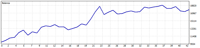
Fig. 7. A Strategy Tester balance graph for the demonstration EA, showing the reflexivity gate firing on a chosen symbol and period rather than a number to take on faith

Conclusion

A Hawkes process turns the vague observation that volatility clusters into a single number you can watch. This article built one in MQL5 from the event train up: a causal threshold extractor on a bar clock, an exponential kernel whose intensity and integral both collapse to O(N), a recursive log-likelihood, and a maximum-likelihood fitter parameterized so that stationarity is a wall rather than a wedge. The branching ratio that comes out is a reflexivity gauge, high when the market is feeding on itself and low when it is not.

What was built, and what you can run:

• A Hawkes library: event extraction, the exponential-kernel intensity and compensator, the recursive log-likelihood, and the MLE fitter with its bound diagnostics.
• Test scripts that verify the kernel, the likelihood, and the fitter inside MQL5, plus a Python cross-check that recomputes everything independently and agrees to rounding.
• An indicator that plots the fitted intensity and the live reflexivity reading, and a demonstration EA that gates on it.
• The Python scripts that simulate event trains and cross-check the compiled library against an independent recomputation.

Two honest limits travel with all of this. The branching ratio is biased low and should be read as ordinal, so treat a rise as more clustering rather than as a calibrated probability. And on an efficient market the correct reading is close to zero: the tool describes the recent past, it does not forecast the future. Used that way, as a reflexivity meter rather than a signal generator, it adds a measurement to the chart that nothing else in the standard toolkit provides.

#	Filename	Type	Description
1	Hawkes.mqh	Include	Facade class CHawkes: price to event train to fit to intensity
2	HawkesData.mqh	Include	Event extraction: the causal k*sigma threshold on a bar clock
3	HawkesKernel.mqh	Include	Exponential kernel: O(N) intensity recursion and closed-form compensator
4	HawkesLikelihood.mqh	Include	Recursive log-likelihood of an event train
5	HawkesFitter.mqh	Include	MLE of (mu, alpha, beta) over (mu, n, beta), grid seed plus Nelder-Mead
6	Hawkes_Test_Kernel.mq5	Script	Checks the O(N) recursion against the brute sum and the integral
7	Hawkes_Test_Likelihood.mq5	Script	Checks the log-likelihood assembly and the Poisson corner
8	Hawkes_Test_Fitter.mq5	Script	Parameter recovery on Ogata-simulated event trains
9	Hawkes_Export_ForCrosscheck.mq5	Script	Exports trains, probe log-likelihoods, and fits for the Python check
10	Hawkes_Scan_Market.mq5	Script	Sliding-window branching-ratio profile on a real chart
11	Hawkes_Intensity.mq5	Indicator	Fitted intensity, event markers, and the reflexivity panel
12	Hawkes_Reflexivity_EA.mq5	Expert	Demonstration: entries gated on reflexivity and intensity (no profit claim)
13	hawkes_simulate.py	Python	Ogata thinning simulator plus independent brute log-likelihood
14	hawkes_ref.py	Python	Statement-for-statement Python mirror of the MQL5 fitter (drives the cross-check)
15	hawkes_crosscheck.py	Python	Cross-check runner: numpy versus the exported MQL5 numbers
16	MQL5.zip	Archive	Archive with all project files in their subfolders; unpack it into the terminal data directory and every file lands in its required location