Time Series Shapelets: Learning a Price Shape, and Testing Whether It Means Anything

Contents

• Introduction
• What a shapelet actually is
• From a price series to a labeled dataset
• The distance primitive
• Scoring a candidate with information gain
• The finder, and the duplicate trap
• Two numbers that keep the library honest
• Calling it
• Verification
• The indicator: plot the rule, not the verdict
• What the shapes say on real data
• Conclusion

Introduction

Most pattern recognition in trading works by describing a shape in advance. You write down what a head and shoulders is, or a flag, or an engulfing candle, and then you scan for it. The description comes from a human, so every disagreement about whether a formation counts is really a disagreement about the description.

Shapelets invert this. You provide the algorithm with labeled windows (here: price windows followed by a meaningful move up or down), it searches all subsequences, and it selects the one that best separates the labels. The output is a short piece of real price history plus a distance cutoff. Ye and Keogh introduced the idea in 2009, and its selling point is interpretability: unlike a neural network, the model is a picture you can put on a chart.

The catch is that a search over thousands of candidates always returns a winner. On a random walk, on shuffled labels, on anything. That is not a flaw in the algorithm, it is what a maximum over many candidates does. So a shapelet library that only finds shapes is dangerous on financial data; it needs to report, in the same breath, how good a shape the same search would have found in noise.

This article covers both parts. First the classic algorithm: z-normalized subsequence distance, an information-gain split to choose the threshold, and a candidate finder. Then what is often missing: a purged hold-out and a block permutation null. Everything compiles and runs in MetaTrader 5, with test scripts and a Python cross-check attached. What you get is a working CShapelets facade, an indicator that draws the learned shape and the decision variable it produces, and a set of measurements that will stop you believing a result that is not there.

What a shapelet actually is

A shapelet is two objects, and keeping them separate is the whole game. The first is a shape: a short subsequence, z-normalized so that only its form matters and not its price level or its volatility. The second is a distance threshold. Together they form a decision stump: measure how far a window sits from the shape, and if that distance is at or below the threshold, predict one class, otherwise the other.

The distance between a shapelet and a longer window is the minimum over all placements. Slide the shape along the window, z-normalize both at every position, take the Euclidean distance, keep the smallest. That answers "how well does this shape fit anywhere in this window", which is exactly the question a pattern is supposed to answer.

The figure below shows both halves on a synthetic dataset where a shape genuinely exists. On the left the learned shape is drawn over the window position where it fits best; on the right every window sits on the distance axis colored by its true class, with the chosen threshold dashed. The separation on the right is the reason the shape on the left is worth looking at.

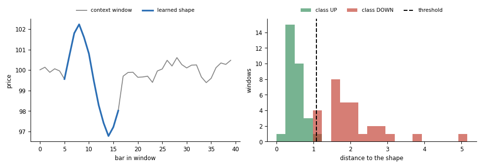
Fig. 1. A shapelet is both halves at once: the learned shape drawn over its best matching position inside a price window, left, and the distance from every window to that shape, colored by class, with the split the information gain chose, right

Two properties follow from z-normalization. The match is invariant to price level, so the same shape is recognized whether gold trades at 2000 or 4000, and invariant to volatility scale, so a quiet version and a violent version of one form are the same shape. That is usually what you want from a pattern, and occasionally it is not: a shapelet cannot tell you a move was large, only that it had a particular form.

The second property cuts deeper than it looks, because the labels built in the next section are defined by the size of the future move relative to volatility. The feature discards scale while the target is constructed from it: the model cannot see scale in what it measures, yet it learns from events that only exist because of scale. That is not an implementation error but a tension in the problem statement, and it is worth holding on to.

From a price series to a labeled dataset

Price does not come labeled, so CShapeletData produces the labels. Every bar with enough history behind it and enough future ahead becomes one example: a context window of the previous Lctx closes, labeled by what happened next.

The label is the sign of the forward log return over horizon bars, but not every move counts. A move only earns a label if it exceeds k times the trailing standard deviation of one bar log returns; anything smaller is dropped as FLAT. Dropping is deliberate: it reduces the chance of the shapelet fitting the shape of noise, and it means a "class UP" window really did precede a move that mattered relative to how the market was moving at the time. It does not remove that chance. Excluding the small moves makes the surviving sample conditional on extreme future changes, which is a selection and not a cleaning, so what the search finds there can still be an artifact of selecting extreme observations rather than a shape that repeats.

An adaptive threshold rather than a fixed one is not a stylistic choice. A fixed pip threshold fires constantly in a volatile week and never in a quiet one, so the two classes would end up describing volatility regimes rather than direction.

One property of that threshold is a choice rather than a derivation, and it is easy to miss. The forward move spans horizon bars, while the threshold is k times the standard deviation of a single bar return. For independent returns the standard deviation of a horizon bar move grows roughly as sqrt(horizon) times sigma, and the code does not apply that factor. So k is in one bar sigma units throughout, and how many UP and DOWN events survive depends on horizon in a way the parameter name does not advertise. Change horizon and expect to retune k.

//+------------------------------------------------------------------+
//| Build labeled windows                                            |
//+------------------------------------------------------------------+
bool CShapeletData::Build(const double &price[], int n,
                          int Lctx, int horizon, double k, int volWin)
  {
   m_count = 0;
   m_cols  = Lctx;
   if(Lctx < 4 || horizon < 1 || n < Lctx + horizon + 2)
     {
      Print("ShapeletData::Build - series too short for the window/horizon");
      return false;
     }
   //--- one-bar log returns (ret[0] = 0)
   double logp[], ret[];
   ArrayResize(logp, n);
   ArrayResize(ret,  n);
   for(int i = 0; i < n; i++)
      logp[i] = MathLog(price[i]);
   ret[0] = 0.0;
   for(int i = 1; i < n; i++)
      ret[i] = logp[i] - logp[i - 1];
   //--- upper bound on the number of windows, allocate once
   int maxRows = n - Lctx - horizon + 1;
   if(maxRows < 1)
      return false;
   ArrayResize(m_rows,   maxRows);
   ArrayResize(m_y,      maxRows);
   ArrayResize(m_endBar, maxRows);
   for(int t = Lctx - 1; t < n - horizon; t++)
     {
      //--- trailing sigma of one-bar returns over [t-volWin+1 .. t]
      int lo = t - volWin + 1;
      if(lo < 1)
         lo = 1;                       // ret[0] is a filler zero
      int cnt = t - lo + 1;
      if(cnt < 2)
         continue;
      double mean = 0.0;
      for(int i = lo; i <= t; i++)
         mean += ret[i];
      mean /= cnt;
      double var = 0.0;
      for(int i = lo; i <= t; i++)
        {
         double d = ret[i] - mean;
         var += d * d;
        }
      var /= cnt;
      double sig = MathSqrt(var);
      if(sig <= SHP_ZEPS)
         continue;
      double fwd = logp[t + horizon] - logp[t];
      double thr = k * sig;
      int lab;
      if(fwd >= thr)
         lab = 1;
      else if(fwd <= -thr)
         lab = 0;
      else
         continue;                     // FLAT -> drop
      //--- copy the raw context window price[t-Lctx+1 .. t]
      ArrayResize(m_rows[m_count].v, Lctx);
      int base = t - Lctx + 1;
      for(int kk = 0; kk < Lctx; kk++)
         m_rows[m_count].v[kk] = price[base + kk];
      m_y[m_count]      = lab;
      m_endBar[m_count] = t;
      m_count++;
     }
   ArrayResize(m_rows,   m_count);
   ArrayResize(m_y,      m_count);
   ArrayResize(m_endBar, m_count);
   return (m_count > 0);
  }

Three details in this function matter later. The trailing sigma window starts at index 1 because ret[0] is a filler zero and would drag the mean. The rows are stored as raw price, not returns, so the shape the reader eventually sees on a chart is a shape in price. And m_endBar records where each row sits on the price axis, as the index of that window's last bar.

That last one looks like bookkeeping and is not. FLAT windows are dropped, so row index 7 is not bar index 7 and the mapping cannot be recovered later. Without m_endBar the library finds a shape but cannot say which bars it came from, which would make an interpretable method uninterpretable.

Two coordinate systems are now in play, so it is worth pinning down which one leaves this class; every later section depends on the answer. m_endBar stores window ends, the finder and the hold-out both want window starts, and CShapeletData does that conversion in exactly one place:

//+------------------------------------------------------------------+
//| Copy each row's first-bar index out                              |
//+------------------------------------------------------------------+
void CShapeletData::GetOrigins(int &out[]) const
  {
   ArrayResize(out, m_count);
   for(int r = 0; r < m_count; r++)
      out[r] = m_endBar[r] - m_cols + 1;
  }

So wherever the rest of this article says origin or rowOrigin, it means a window's first bar, and origin[r] + cols - 1 recovers the end. That is why the purge below writes origin[cutIdx] + cols - 1 for a boundary bar while the de-duplication test writes rowOrigin[...] + srcStart for a candidate's first bar: both read one axis. Passing ends where starts are expected would shift every bar span and every purge boundary by Lctx minus one.

The distance primitive

Everything downstream is built on one operation: the minimum z-normalized distance from a shape to a series. Computing it naively means z-normalizing every window from scratch, O(m) work per placement, and the standard fix is to precompute a rolling mean and standard deviation for every window position in one pass.

The obvious way is a prefix sum of the values and a prefix sum of the squares, then var = sum2/m - mean^2. That formula is correct in exact arithmetic and dangerous in floating point: when the price level dwarfs the bar-to-bar spread, which is the normal state of a financial series, sum2/m and mean^2 are two large and nearly equal numbers, and subtracting them throws away most of the significant digits. The fix is one extra pass, subtracting the series mean before accumulating. A constant shift changes no variance, so the result is exact, just conditioned very differently.

//+------------------------------------------------------------------+
//| Rolling mean and population std via prefix sums (O(n))           |
//+------------------------------------------------------------------+
void CShapeletDistance::RollingStats(const double &series[], int n, int m,
                                     double &mu[], double &sig[])
  {
   int L = n - m + 1;
   if(L <= 0)
     {
      ArrayResize(mu, 0);
      ArrayResize(sig, 0);
      return;
     }
   //--- Shift by the series mean before accumulating. A constant shift changes
   //--- no variance, so this is exact, but it avoids the cancellation in
   //--- s2/m - mean^2 when the price LEVEL dwarfs the bar-to-bar spread.
   double c = 0.0;
   for(int i = 0; i < n; i++)
      c += series[i];
   c /= n;
   double cs[], cs2[];
   ArrayResize(cs,  n + 1);
   ArrayResize(cs2, n + 1);
   cs[0] = 0.0;
   cs2[0] = 0.0;
   for(int i = 0; i < n; i++)
     {
      double v = series[i] - c;
      cs[i + 1]  = cs[i]  + v;
      cs2[i + 1] = cs2[i] + v * v;
     }
   ArrayResize(mu,  L);
   ArrayResize(sig, L);
   double invm = 1.0 / m;
   for(int i = 0; i < L; i++)
     {
      double s  = cs[i + m]  - cs[i];
      double s2 = cs2[i + m] - cs2[i];
      double mean = s * invm;
      double var  = s2 * invm - mean * mean;
      if(var < 0.0)
         var = 0.0;
      mu[i]  = mean + c;             // back to original units
      sig[i] = MathSqrt(var);
     }
  }

This is not a hypothetical, and the library's own Level 1 test is what makes it visible. It compares MinDistZ against a two-pass brute-force implementation at a 1e-09 tolerance; with the centering in place the worst error over forty five checks is 6.2e-15. ZNorm and the brute force reference already used the stable two-pass form, which is why a prefix-sum RollingStats would disagree with them and why the test catches it rather than agreeing with its own mistake.

With the rolling statistics in hand, the match itself is a sweep with one optimization that matters. While scanning placements we carry the best squared distance found so far, and the moment a placement's running total exceeds it we stop accumulating. The minimum is still exact, because only placements that were already provably worse get cut short.

//+------------------------------------------------------------------+
//| Minimum z-norm distance, early-abandoned                         |
//+------------------------------------------------------------------+
double CShapeletDistance::MinDistZ(const double &zs[], int m,
                                   const double &series[], int n,
                                   const double &mu[], const double &sig[],
                                   int &pos, double bsf)
  {
   int L = n - m + 1;
   pos = -1;
   double best2 = bsf * bsf;          // compare squared distances
   if(bsf >= DBL_MAX)
      best2 = DBL_MAX;
   for(int j = 0; j < L; j++)
     {
      double sg = sig[j];
      double mj = mu[j];
      double acc = 0.0;
      bool abandoned = false;
      if(sg <= SHP_ZEPS)
        {
         //--- flat window: its z-shape is all zeros, so the squared distance
         //--- is sum(zs^2). Matches the prototype's znorm(flat)=zeros rule.
         for(int k = 0; k < m; k++)
            acc += zs[k] * zs[k];
        }
      else
        {
         double inv = 1.0 / sg;
         for(int k = 0; k < m; k++)
           {
            double zw = (series[j + k] - mj) * inv;
            double d  = zw - zs[k];
            acc += d * d;
            if(acc >= best2)          // early abandon: this window can't win
              {
               abandoned = true;
               break;
              }
           }
        }
      if(!abandoned && acc < best2)
        {
         best2 = acc;
         pos = j;
        }
     }
   if(pos < 0)                        // every window abandoned against bsf
      return bsf;
   return MathSqrt(best2 < 0.0 ? 0.0 : best2);
  }

The population standard deviation, dividing by m rather than m minus 1, is deliberate. It makes the sum of squared z values exactly m, which makes the identity d^2 = 2m(1 - rho) exact, where rho is the Pearson correlation between the shape and the window. That is an entirely independent formula for the same quantity, and the cross-check uses it as an oracle.

Scoring a candidate with information gain

A candidate subsequence produces one distance per row. To score it, sort those distances and treat every midpoint between two consecutive distinct values as a possible threshold. Each threshold splits the rows into a near group and a far group, and the best one maximizes information gain: the parent entropy minus the weighted entropies of the two groups. Entropy depends only on the class counts, so the sweep carries a running count of class 1 on the left rather than recomputing from scratch, which is what makes scoring a candidate O(n log n) for the sort rather than O(n^2).

//+------------------------------------------------------------------+
//| Optimal split of ALREADY-SORTED distances                        |
//+------------------------------------------------------------------+
SShapeletSplit CShapeletInfoGain::OptimalSplitOrdered(const double &ds[],
                                                      const int &ys[], int n)
  {
   SShapeletSplit best;
   if(n < 2)
      return best;
   //--- total class-1 count and parent entropy
   int total1 = 0;
   for(int i = 0; i < n; i++)
      if(ys[i] != 0)
         total1++;
   double hParent = EntropyCount(total1, n);
   //--- sweep the split point, accumulating the left class counts
   int leftC1 = 0;
   for(int i = 0; i < n - 1; i++)
     {
      if(ys[i] != 0)
         leftC1++;
      if(ds[i] == ds[i + 1])
         continue;                   // cannot split between equal distances
      int nL = i + 1;
      int nR = n - nL;
      double hL = EntropyCount(leftC1, nL);
      double hR = EntropyCount(total1 - leftC1, nR);
      double gain = hParent - ((double)nL / n) * hL - ((double)nR / n) * hR;
      double margin = ds[i + 1] - ds[i];
      bool better = gain > best.gain + 1e-15 ||
                    (MathAbs(gain - best.gain) <= 1e-15 && margin > best.margin);
      if(better)
        {
         best.gain       = gain;
         best.threshold  = 0.5 * (ds[i] + ds[i + 1]);
         best.classBelow = (leftC1 * 2 >= nL) ? 1 : 0;
         best.margin     = margin;
        }
     }
   return best;
  }

Notice what this function does not do: it does not sort. The sort lives in a separate SortIndex call, and that separation looks like tidiness while actually being the performance decision that pays for the null in the next section. A candidate's distances do not depend on the labels, so one sorted order can be re-scored against many label vectors in O(n) each, which is what makes twenty permutations cost a fraction of a fit instead of twenty fits.

Ties on gain are broken by the wider margin, so when two thresholds separate the classes equally well the cut sits in the middle of the wider gap. Small thing, and it makes the resulting rule noticeably more stable.

The finder, and the duplicate trap

The finder enumerates candidates: every subsequence of every allowed length, taken from every row, subsampled by a step parameter to keep the cost bounded. Each is scored, and the best is the shapelet. Asking for the top k gives you several shapes to vote with, and the classic rule for keeping them different is remove_similar: reject a candidate that overlaps an already accepted one.

That rule is written for datasets whose rows are independent series. Here they are not. The rows are sliding context windows of one price series, so consecutive rows share all but one bar, and the same physical subsequence appears as row r at offset s, row r+1 at offset s-1, row r+2 at offset s-2, and so on. Every copy has a different row index, so an overlap test on row indices passes all of them.

The result is a top k that is one shape repeated k times. The left panel below shows the four shapes the naive rule keeps on a random walk: the same curve four times, all traced back to bar 223. The right panel is the same search with the fixed rule.

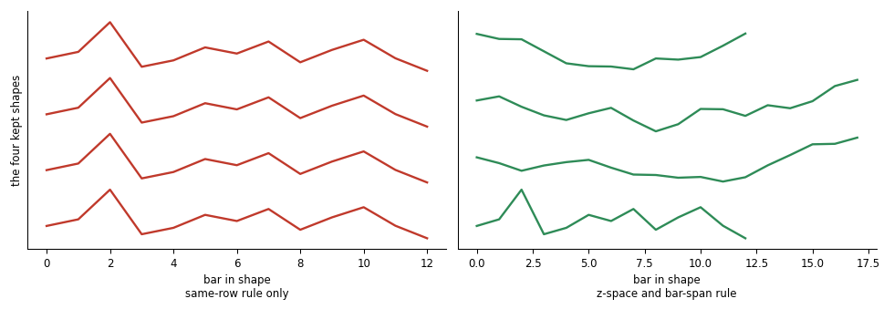
Fig. 2. The four kept shapes under the two de-duplication rules: comparing row indices keeps four copies of one subsequence, left, while the z-space and bar-span test keeps four shapes that are genuinely different, right

This is worse than cosmetic. Any vote across those four shapes is unanimous by construction, so a confidence figure computed from them reads 1.00 whatever the market is doing, and a gate built on that confidence does nothing at all.

The fix rejects duplicates in the two coordinate systems that actually mean something. Absolute bar space, using the row origins that CShapeletData now records, catches the same physical bars reached through a different row. Z-space catches the same form found somewhere else entirely, with one limit worth naming: the z-space test compares only candidates of equal length, as the c.len == sh.len guard in the listing shows. A similar form at a different length is not caught and survives as a separate shapelet, so the protection against repeated shapes is narrower than "the same form, wherever it came from" suggests.

//+------------------------------------------------------------------+
//| Is this candidate the same shape as one already accepted?        |
//+------------------------------------------------------------------+
bool CShapeletFinder::IsDuplicate(SShpRow &rowsArr[], SShpCand &c,
                                  SShapelet &sh, const int &rowOrigin[],
                                  bool removeSimilar)
  {
   //--- classic rule: overlapping spans of the SAME row
   if(removeSimilar &&
      Overlap(c.srcSeries, c.srcStart, c.len,
              sh.srcSeries, sh.srcStart, sh.len))
      return true;
   //--- the same physical bars reached through a different row
   if(removeSimilar && ArraySize(rowOrigin) > 0)
     {
      int a = rowOrigin[c.srcSeries] + c.srcStart;
      int b = rowOrigin[sh.srcSeries] + sh.srcStart;
      if(!(a + c.len <= b || b + sh.len <= a))
         return true;
     }
   //--- the same SHAPE at the same length, wherever it came from
   if(c.len == sh.len)
     {
      double zc[];
      if(!CShapeletDistance::ZNorm(rowsArr[c.srcSeries].v, c.srcStart, c.len, zc))
         return false;
      double acc = 0.0;
      for(int t = 0; t < c.len; t++)
        {
         double d = zc[t] - sh.z[t];
         acc += d * d;
        }
      if(MathSqrt(acc) < SHP_DUP_TOL * MathSqrt(2.0 * c.len))
         return true;
     }
   return false;
  }

The tolerance is a fraction of sqrt(2L), a quantity easy to call the maximum and be wrong about. Under population normalization every z-normalized vector of length L has norm sqrt(L), so the identity d^2 = 2L(1 - rho) gives sqrt(2L) at rho = 0 and 2*sqrt(L) at rho = -1. sqrt(2L) is therefore the distance between an uncorrelated pair; the genuine maximum is 2*sqrt(L), from an exactly anticorrelated pair. The uncorrelated distance is the better yardstick anyway, since two shapes worth calling different should be somewhat uncorrelated rather than merely short of being mirror images, and either scale grows with sqrt(L), which is what keeps one tolerance meaningful across every candidate length.

De-duplication sweeps the remaining candidates once after each acceptance and retires every copy of the shape just taken, which keeps the cost at O(count) per pick. Re-scanning after each individual rejection would be O(count) per duplicate, and on sliding windows a popular shape has thousands of duplicates.

What de-duplication does not buy is independence. It makes the kept shapelets different from one another, but all of them remain maxima over the same candidate scan on the same rows, so their errors stay correlated. The fraction that agree on a row is a spread of opinion among related voters, not a probability that the row belongs to that class.

One more selection problem is worth naming, because fixing de-duplication does not fix it. Ranking the top k by gain alone can return shapes that all predict the same class: on a daily gold window with 127 up rows against 56 down, all five kept shapelets predicted up, leaving no down shape to display. FindTopKEx therefore also returns the strongest candidate of each class separately, which costs nothing because the candidates are already scored.

Two numbers that keep the library honest

Here is the part that decides whether any of the above is worth running on price data.

Training accuracy is not evidence. Classifying the rows a model was fitted on is close to meaningless for a shapelet, because the shape is literally a subsequence cut out of one of those rows, which therefore scores a distance of zero, and it was selected as the maximum over thousands of candidates on those same rows. Measured on a random walk, in-sample accuracy reads 0.687 while a proper hold-out reads 0.533 against a majority class baseline of 0.644. On real gold the pair is 0.661 and 0.500.

So CShapelets::Fit runs a second fit on the older rows only and scores the newest rows with it. A plain split leaks: rows either side of the cut share bars and their labels share forward returns, so a shape learned just before the cut has partially seen the data just after it. The training side is purged, dropping any row whose window or horizon crosses the boundary.

//+------------------------------------------------------------------+
//| Purged hold-out: fit on the older rows, score the newest ones    |
//|                                                                  |
//|  Rows are sliding windows, so the rows either side of the cut    |
//| share bars and their labels share forward returns. A plain split |
//|  therefore leaks. Every training row whose window or horizon can |
//|  touch the validation side is dropped - the standard purge, and  |
//|  the reason ValAccuracy() is worth reading at all.               |
//+------------------------------------------------------------------+
void CShapelets::Holdout(SShpRow &rowsArr[], int &y[], const int &origin[],
                         int rows, int cols)
  {
   m_valAcc = -1.0; m_valN = 0; m_valBase = 0.0;
   if(m_p.valFrac <= 0.0 || m_p.valFrac >= 1.0)
      return;
   int cutIdx = (int)((1.0 - m_p.valFrac) * rows);
   if(cutIdx < 8 || rows - cutIdx < 4)
      return;                              // not enough rows to say anything
   //--- purge: a training row must end before the validation window begins
   int cutBar = origin[cutIdx] + cols - 1;
   int purge  = cols + m_p.horizon;
   SShpRow trRows[];
   int trY[], trOrigin[];
   ArrayResize(trRows, cutIdx);
   ArrayResize(trY, cutIdx);
   ArrayResize(trOrigin, cutIdx);
   int nTr = 0;
   for(int r = 0; r < cutIdx; r++)
     {
      if(origin[r] + cols - 1 > cutBar - purge)
         continue;
      ArrayResize(trRows[nTr].v, cols);
      for(int c = 0; c < cols; c++)
         trRows[nTr].v[c] = rowsArr[r].v[c];
      trY[nTr]      = y[r];
      trOrigin[nTr] = origin[r];
      nTr++;
     }
   if(nTr < 8)
      return;
   ArrayResize(trRows, nTr);
   ArrayResize(trY, nTr);
   ArrayResize(trOrigin, nTr);
   SShapelet vsh[];
   int nLen = ArraySize(m_p.lengths);
   int nv = CShapeletFinder::FindTopK(trRows, nTr, cols, trY, m_p.lengths, nLen,
                                      m_p.step, m_p.topK, m_p.removeSimilar,
                                      trOrigin, vsh);
   if(nv <= 0)
      return;
   //--- score the untouched newest rows with that model
   int correct = 0, up = 0;
   for(int r = cutIdx; r < rows; r++)
     {
      int agree = 0;
      for(int j = 0; j < nv; j++)
         if(CShapeletFinder::Predict(vsh[j], rowsArr[r].v, cols) == 1)
            agree++;
      int cls;
      if(agree * 2 > nv)      cls = 1;
      else if(agree * 2 < nv) cls = 0;
      else                    cls = CShapeletFinder::Predict(vsh[0], rowsArr[r].v, cols);
      if(cls == y[r])
         correct++;
      if(y[r] != 0)
         up++;
     }
   m_valN   = rows - cutIdx;
   m_valAcc = (double)correct / m_valN;
   double pUp = (double)up / m_valN;
   m_valBase = MathMax(pUp, 1.0 - pUp);
  }

Two limits bound how hard that number can be read. The validation rows are still sliding windows of one series, so they overlap and their labels share forward returns; m_valN counts rows, not independent observations, and a significance level computed from it would be overstated. And the comparison is against the majority class rate alone, a low bar that ignores label autocorrelation, so a rule that merely persisted the previous label is not among the things being beaten, nor is any other simple temporal rule. Beating ValBaseline is a classification result on dependent rows.

Information gain is a selection statistic, so an absolute threshold on it is unreliable. The top gain is a maximum over thousands of candidates, and it shrinks as the dataset grows. The reason is not the maximization itself, which is worth getting right: a maximum over more draws from one fixed distribution can only rise or stay level. What moves is the distribution being drawn from. Entropy estimated from class counts carries a finite sample bias, an information gain built from those estimates is biased upward, and both biases shrink as rows grow, which also leaves less room for a single cut to separate them by luck. The figure below measures the result: the top gain a full search finds on pure random walks, at five dataset sizes, with no signal anywhere.

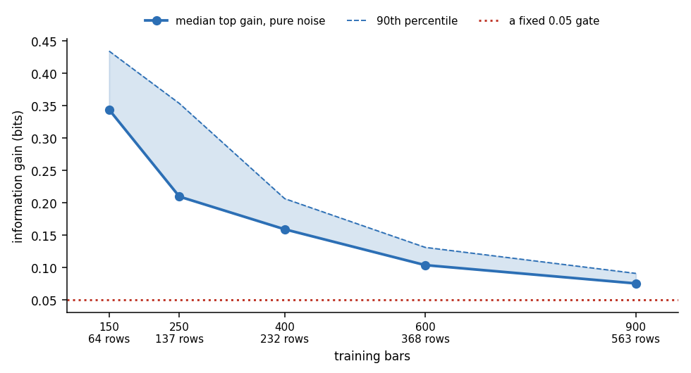
Fig. 3. The best information gain a full search finds on pure random walks falls from 0.34 at 150 bars to 0.08 at 900, so a fixed 0.05 gate is cleared by noise alone at every size

The median falls from 0.344 at 150 bars to 0.075 at 900 bars, so a fixed gate of 0.05, which sounds conservative, is cleared by pure noise at every size tested. The conclusion is about the kind of threshold rather than the number. A cut that takes no account of the sample size, of how many candidates were enumerated, and of the shape of the null distribution is unreliable, because the same absolute value means something different at every training length. A threshold that did account for those three would be a different object, and that object is the null below.

The alternative is a relative question: does this gain beat the gain the same search finds after the labels are shuffled? That is a permutation null, cheap here because the distances do not depend on the labels. ScoreCandidates sorts each candidate once and re-scores it against every permuted label vector, so twenty permutations cost a fraction of the fit rather than twenty fits.

Be precise about what this null breaks. Shuffling the labels destroys the window to label relationship and leaves the price windows, with all of their autocorrelation and trend, exactly as they were. It is a null for that relationship, not a model of market noise; the noise question is answered separately by Fig. 3 above and by the matched random walk quoted later, where the prices rather than the labels are replaced.

The shuffle itself needs care, and getting it wrong is worse than having no null. Adjacent windows share their forward return horizon, so real labels arrive in runs: 21 runs across 112 gold rows, where an independent draw would give about 56. Shuffling labels one at a time destroys those runs and lowers the noise floor, making the real gain look significant against a floor that is too low.

//+------------------------------------------------------------------+
//| nPerm BLOCK-shuffled copies of the labels, row-major [p*rows+r]  |
//|                                                                  |
//|  Whole blocks of consecutive labels are permuted, never single   |
//|  labels, so the run structure survives the shuffle. See the note |
//|  on CShapelets for what an iid shuffle does instead (it invents  |
//|  significance on pure noise, 5 walks out of 5).                  |
//+------------------------------------------------------------------+
void CShapelets::BuildPermutations(const int &y[], int rows, int nPerm,
                                   int &yPerm[])
  {
   //--- block length: given, or twice the mean label run
   int b = m_p.permBlock;
   if(b <= 0)
     {
      int nRuns = 1;
      for(int r = 1; r < rows; r++)
         if(y[r] != y[r - 1])
            nRuns++;
      b = 2 * (int)MathCeil((double)rows / (double)nRuns);
     }
   if(b < 1)    b = 1;
   if(b > rows) b = rows;
   int nb = (rows + b - 1) / b;
   int order[];
   ArrayResize(order, nb);
   ArrayResize(yPerm, rows * nPerm);
   for(int p = 0; p < nPerm; p++)
     {
      for(int i = 0; i < nb; i++)
         order[i] = i;
      //--- Fisher-Yates over the BLOCK order
      for(int i = nb - 1; i > 0; i--)
        {
         int j = (int)(NextRand() % (uint)(i + 1));
         int t = order[i];
         order[i] = order[j];
         order[j] = t;
        }
      //--- lay the blocks back down in the shuffled order
      int off = p * rows;
      int w = 0;
      for(int i = 0; i < nb && w < rows; i++)
        {
         int src = order[i] * b;
         for(int q = 0; q < b && w < rows; q++)
           {
            if(src + q >= rows)
               break;
            yPerm[off + w] = y[src + q];
            w++;
           }
        }
      //--- a short trailing block can leave a gap; fill it in order
      for(int r = w; r < rows; r++)
         yPerm[off + r] = y[r];
     }
  }

The block length defaults to twice the mean label run, computed from the data, and the figure below shows why it matters. On the left, the two null distributions on one random walk: the independent shuffle floor sits near 0.064 and the block shuffle floor near 0.171, a ratio of 2.7. On the right, six independent random walks containing no signal at all, with the percentile the real gain reaches in its own null under each shuffle.

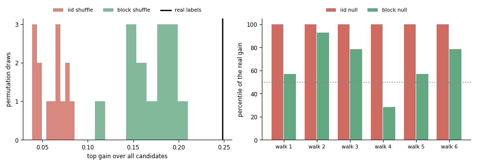
Fig. 4. An independent shuffle sets a lower floor than a block shuffle, left, and puts the real gain of six pure random walks at the 100th percentile every time, right, where the block null scatters between 29 and 93

The independent shuffle puts the real gain at the 100th percentile on all six walks: six false positives out of six, on data with nothing in it. Six simulations will not pin down a false positive rate as a property of the method, and it should not be read as one, but a null that fails every draw it was given is unusable as a screen. The block shuffle gives 57, 93, 79, 29, 57 and 79, scattered around the middle, which is what a usable null on pure noise should look like.

Usable rather than calibrated is the right word. A block shuffle keeps runs of identical labels inside a block and breaks the dependence at every block boundary, so the structure it preserves is partial by construction, and the block length is itself estimated from the label runs, which is not stable on a hundred-odd rows. How far these percentiles move with the block length and with the number of permutations is not measured here, so this is a screen whose own sensitivity is unknown.

Important: the block null is a screen, not a proof. It still reads high on some pure noise draws, as the 93rd percentile above shows. A matched random walk resample of the same symbol is a useful second control rather than a definitive one, because what it reports depends on the random walk model chosen, on the volatility fed to it, and on the return distribution assumed. The single number most worth trusting is the purged hold-out edge.

Calling it

All of the above sits behind one facade: fill in a parameter struct, hand over an oldest first price array, read the results. The excerpt below comes from the honesty test script.

   BuildWalk(price, InpBars, 0.0034);
   SShapeletParams p;
   p.Lctx = 40; p.horizon = 5; p.k = 1.0; p.volWin = 100;
   p.step = 2; p.topK = 4; p.removeSimilar = true;
   p.valFrac = 0.30; p.nPerm = 20; p.permBlock = 0; p.seed = 777;
   ArrayResize(p.lengths, 4);
   p.lengths[0] = 10; p.lengths[1] = 13; p.lengths[2] = 15; p.lengths[3] = 18;
   CShapelets sh;
   sh.SetParams(p);

The candidate lengths are supplied explicitly rather than derived, because the right range depends on what you are looking for: ten to eighteen bars on H1 is a shape that forms over a session, while the same numbers on D1 form over weeks. step subsamples candidate start positions and is the main speed control. valFrac and nPerm switch on the two honesty measurements, and zero turns either off.

After a successful Fit the interesting reads are TopGain, GainPercentile and PValue for how the shape compares to its own null, ValAccuracy against ValBaseline for the out-of-sample edge, and GetBestOfClass for the strongest shape predicting each direction. Each returned shapelet carries its own z array, its threshold, and the srcBar it was cut from.

nPerm sets the resolution of the first two, and the default is coarse. The p-value is (1 + #{null >= real}) / (nPerm + 1), so at nPerm = 20 the smallest it can return is 1/21, about 0.048. That separates a gain sitting mid-null from one that tops it, which is all this article asks of it, and falls well short of supporting significance at any conventional level: a reading near the floor means only that 20 draws could not see past it. Raise nPerm if you need a p-value rather than a screen; the cost is linear in it and small next to the fit.

The cost is dominated by the candidate scan, which is roughly quadratic in the number of labeled rows. Measured on 700 bars producing 450 rows, a bare fit takes 7.4 seconds, the hold-out adds 41 percent, which is about what a second fit over 70 percent of the rows should cost, and twenty permutations add 46 percent on top of that.

Verification

The library is checked at three levels, and the attached scripts run all of them. Level 1 checks the primitives against independent implementations in the same script: the minimum z-normalized distance against a two-pass brute-force, the same distance against the correlation identity d^2 = 2m(1 - rho), and the raw distance against a direct sweep. Level 2 checks behavior that only emerges from the assembled parts: recovery of a planted shape, and the four properties of the honesty machinery. Level 3 exports datasets and MQL5 results to CSV, and a Python script re-derives them with numpy and pyts.

The Level 3 finder check is the strongest, because it is not a mirror of the MQL5 code. The Python reference is an independent brute force enumeration written from the algorithm description, and it must select the same shapelet: same source row, same offset, same length, same gain, same threshold. Two independent implementations of one deterministic algorithm agreeing exactly is much better evidence than a numeric tolerance.

Exact agreement is also easy to over-read, so it is worth bounding. It shows the algorithm is implemented as specified and reproduces across two languages. It says nothing about whether the labeling scheme, the null model, the purge or the significance tests are statistically adequate for a price series; those are the subject of the previous section and of the real data section below.

Level	Script	What it proves	Result
1	Shapelet_Test_Distance.mq5	Distance against brute force and the correlation identity	45 PASS, 0 FAIL (worst error 6.2e-15)
1	Shapelet_Test_InfoGain.mq5	Entropy and the optimal split on hand verified cases	8 PASS, 0 FAIL
2	Shapelet_Test_Finder.mq5	Recovery of a planted shape	18 PASS, 0 FAIL
2	Shapelet_Test_Transform.mq5	Feature matrix and the facade end to end	9 PASS, 0 FAIL
2	Shapelet_Test_Honesty.mq5	De-duplication, provenance, hold-out, and the null	16 PASS, 0 FAIL
3	shapelet_crosscheck.py	MQL5 output against numpy, pyts, and an independent finder	26 PASS, 0 FAIL

Two assertions in the honesty test are worth calling out, because they check claims made earlier in this article. One asserts that the kept shapelets occupy disjoint bar spans and that equal length pairs exceed the duplicate tolerance, which is the de-duplication fix. Another asserts that running with and without the permutation null selects the identical shapelets, so the null measures the fit without disturbing it.

The indicator: plot the rule, not the verdict

The natural way to display a classifier is an arrow on every bar where it fires. For a shapelet that is the wrong choice, for a reason specific to how the threshold is chosen. The information gain split cuts the distance distribution wherever entropy drops the most, which gives it no reason to land in a rare tail, and usually it does not: on gold H1 the best pre-DOWN shape sits below its threshold on 69 percent of scanned bars. That is not a signal, it is wallpaper, about a hundred arrows on a 150 bar screen.

For diagnosing a shapelet rule, the decision variable tells you more than the decision does. Shapelet_Classifier.mq5 therefore plots d(t), the distance from the window ending at each bar to the learned shape, as a curve in a subwindow, with the rule's own threshold as a second line. Where the curve dips under its line the shape is present, and how deeply it dips is how good the match is, which an arrow cannot express.

//+------------------------------------------------------------------+
//| Retrain on cadence, then measure d(t) over the display window    |
//+------------------------------------------------------------------+
   //--- d(t) across the display window, plus each rule's threshold
   double ctx[];
   ArrayResize(ctx, InpLctx);
   SClassStat stUp, stDn;
   stUp.have = haveUp; stDn.have = haveDn;
   int bestUpStart = -1, bestDnStart = -1;
   double bestUp = DBL_MAX, bestDn = DBL_MAX;
   for(int b = displayStart; b <= endBar; b++)
     {
      int base = b - InpLctx + 1;
      if(base < 0)
         continue;
      for(int k = 0; k < InpLctx; k++)
         ctx[k] = close[base + k];
      if(haveUp)
        {
         int pos;
         double d = CShapeletFinder::Match(shUp, ctx, InpLctx, pos);
         UpDistBuf[b] = d;
         UpThrBuf[b]  = shUp.threshold;
         stUp.scanned++;
         stUp.dmin = MathMin(stUp.dmin, d);
         stUp.dmax = MathMax(stUp.dmax, d);
         stUp.dnow = d;                       // last closed bar wins the loop
         if(d <= shUp.threshold)
            stUp.fired++;
         if(d < bestUp) { bestUp = d; bestUpStart = base + pos; }
        }
     }

That is the measuring core of OnCalculate, excerpted; the retrain cadence and the drawing sit above and below it in the same function. The loop also collects the range of d the panel needs. It runs only over closed bars, and every distance comes from the window ending at that bar, so the reading is causal.

The model is trained on bars strictly older than the display window, so no displayed bar and no displayed label entered the fit. That cut needs more care than it first appears: a displayed distance comes from the context window ending at that bar, so if training ends right where the display begins, the first Lctx minus one displayed bars still overlap the training range and a shape taken from the end of training matches its own source bars at distance zero. The indicator therefore holds out a further Lctx plus horizon bars between the two windows, the same purge the hold-out split uses. Since the deepest a displayed context reaches is Lctx minus one bars back, that gap closes the overlap by construction rather than by luck. The hold-out and the null are switched off here, because both cost a second fit and a chart has to stay responsive; those numbers belong to a script run.

On the main chart the indicator draws two objects: a box around the bars the shape was cut from, which is what srcBar is for, and the shape itself over its best matching window in view. The gap between that template and the candles under it is the distance the subwindow plots. The box always sits left of the displayed range, since the shape is always cut from training bars, so seeing both at once takes a zoomed out chart.

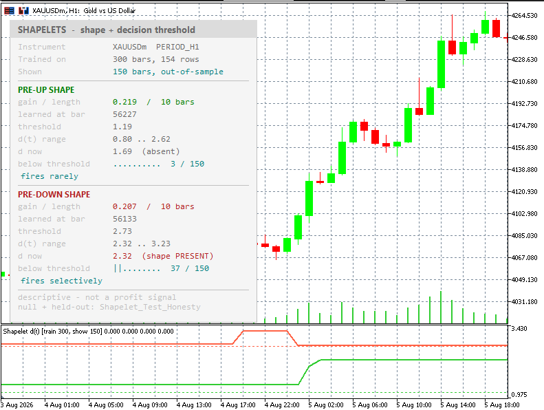
Fig. 5. Shapelet_Classifier on gold H1: in the subwindow each class carries its own distance curve and its own dotted threshold, and the panel reports gain, source bar, threshold, the observed range of d and the fired fraction for both shapes

The capture is XAUUSDm H1, trained on the 300 bars ending 45 bars before the displayed 150, which gave 154 labeled rows. Both classes found a shape of 10 bars, at gain 0.219 and 0.207. Read each dotted line against its own curve and the subject of the next section is already on screen. The pre-UP threshold at 1.19 sits near the floor of its observed range of 0.80 to 2.62, so that rule fires on 3 bars out of 150; the pre-DOWN threshold at 2.73 sits inside a much narrower range of 2.32 to 3.23 and fires on 37. Neither is a signal. Each is a boundary chosen to split one distance distribution and then applied to another, and the panel grades them in its own words: fires rarely for the first, fires selectively for the second.

154 rows is a small training set for a search this wide, and Fig. 3 is the reason to say so plainly: at 150 bars the best gain found on pure random walks ran to 0.34, above both gains quoted here. With a few hundred rows and thousands of candidates scored against them, the chance that a top gain is an accidental maximum stays high, and the null checks that chance rather than removing it. The information gain criterion is least stable exactly where a chart wants to use it.

What the shapes say on real data

The library was run on gold, on H1 and D1, training on 300 bars, holding out the next 45 and displaying the 150 after that. The numbers below come from Shapelet_Verify_Indicator, which drives the indicator through iCustom and reads its buffers back, so they are the plotted curves themselves. They were read one bar after the capture above, which is why the H1 pre-UP count here is 2 where the panel showed 3. The distances all sit inside their theoretical box of 2*sqrt(L) and both classes produce a curve. The mechanics work; the reading is another matter.

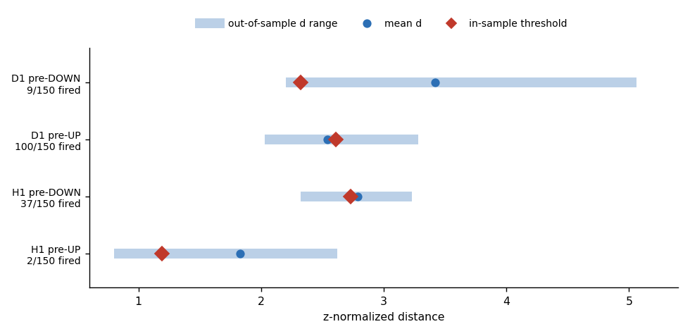
Fig. 6. Each bar is the range of distances actually observed out-of-sample and the diamond is the threshold the fit chose in-sample; the depth at which the diamond lands is what decides whether the rule marks 2 bars in 150 or 100

Every diamond now lands inside its bar, which the pre-purge run did not manage, so the question is no longer whether the rules can fire but where inside the range the boundary falls. On H1 the pre-UP threshold of 1.19 sits near the floor of a 0.80 to 2.62 range and fires on 2 bars out of 150; on D1 the pre-UP threshold of 2.61 sits almost exactly on the mean of the new distances, 2.54, and fires on 100. The same procedure, on the same instrument, produced a rule marking one bar in 75 and a rule marking two bars in three.

A boundary landing on the mean of the distances it is applied to splits them roughly in half, which makes it useless as a rule. That is worth separating from a stronger claim it does not support: a misplaced threshold says nothing on its own about whether d(t) carries information, since the distance could still track the next move perfectly well with the cut somewhere else. The evidence for absence is the next paragraph's, not this one's. What this one shows is a misplaced cut, and marking two bars in three is the same wallpaper the arrows were accused of earlier. The threshold is not a property of the shape but of the particular distances the fit happened to see, and when those distances move, the same shape becomes a rule that almost never fires or one that fires almost always.

This is the argument for plotting the decision variable alongside the decision rather than in place of it. With arrows alone you would see a nearly bare screen on one chart and marks on two bars in three on the other, and could read either as a market state; with a curve and a level you can see the level is in the wrong place. That is a diagnostic preference and not a substitute, because trading needs a discrete or probabilistic criterion in the end, and this library offers none better than the information gain cut. Building one would mean calibrating d(t) against forward returns on held-out rows rather than against the training labels.

The two nulls agree with that verdict. On gold the block permutation null puts the real gain at the 27th percentile, a matched random walk null puts it at the 33rd, and the purged hold-out gives an edge of -0.147, meaning its accuracy came in 14.7 points below the majority class rate. Edge there is a classification quantity and nothing more: it counts directions called right, and takes no account of how large each move was, of spread, commission or slippage, or of any asymmetry between wins and losses. A positive one would not have been a trading result either. A shape was found, and it was worth about as much as noise.

None of that is a defect in the implementation, and it is worth being precise about where the limit lies. On synthetic data where a shape genuinely drives the labels, the same code recovers it with an out-of-sample edge of +0.375 at high signal to noise, decaying smoothly as noise rises. The machinery works on that problem, which is narrower than it sounds: recovering a planted shape shows the search, the split and the hold-out do what they claim when a shape is there to be found, not that this labeling scheme and this validation procedure are right for a financial series. What the gold result adds is that on bar close data most k sigma moves are not preceded by a repeating shape of the kind this search can represent.

That is also why no Expert Advisor ships with this article. The gates such an EA would need, a minimum gain, a minimum training accuracy, a vote confidence, were all measured and all turned out to be satisfied by noise. Publishing a trading system on top of that would mean dressing up a null result.

Conclusion

You now have a complete Time Series Shapelet implementation for MetaTrader 5 that learns an interpretable shape from labeled price windows, reports the threshold that turns it into a rule, and tells you how much of what it found is noise.

• A z-normalized subsequence distance with early abandoning and numerically conditioned rolling statistics, verified against a brute force implementation and against the correlation identity to 6.2e-15.
• An information gain split that yields both a threshold and the class predicted on the near side, with the sort separated from the sweep so the null is cheap.
• A finder that enumerates and ranks candidates, rejects duplicates in bar space and in z-space, records where each shape came from, and returns the strongest shape of each class.
• A purged hold-out that reports an honest out-of-sample accuracy against its majority class baseline.
• A block permutation null that measures how good a shape the same search finds when the labels carry no information, with the block length taken from the label runs.
• An indicator that plots the decision variable and its threshold out-of-sample, and marks the bars the shape was learned from.

The measurement that generalizes beyond this library is the one in the null section. The best information gain over a candidate search on pure noise runs from about 0.34 at 150 training bars to about 0.08 at 900. A threshold on that quantity chosen without reference to the sample size, the number of candidates and the null distribution is cleared by noise at some dataset size, which means a pattern search that does not carry its own null will always find a pattern. Build the null in at the same time as the search, not afterward.

#	Filename	Type	Description
1	ShapeletDistance.mqh	Include	Minimum z-normalized subsequence distance, rolling statistics, early abandoning
2	ShapeletInfoGain.mqh	Include	Entropy and the optimal information gain split of a distance vector
3	ShapeletFinder.mqh	Include	Candidate enumeration, scoring, de-duplication, and the permutation null pass
4	ShapeletData.mqh	Include	Price series to labeled context windows with bar provenance
5	ShapeletTransform.mqh	Include	Series to shapelet distance feature vectors
6	Shapelets.mqh	Include	CShapelets facade: fit, vote, purged hold-out, and null summaries
7	Shapelet_Classifier.mq5	Indicator	Distance curves with thresholds, provenance box, and the learned shape on price
8	Shapelet_Test_Distance.mq5	Script	Level 1: distance against brute force and the correlation identity
9	Shapelet_Test_InfoGain.mq5	Script	Level 1: entropy and split on hand verified cases
10	Shapelet_Test_Finder.mq5	Script	Level 2: planted shape recovery
11	Shapelet_Test_Transform.mq5	Script	Level 2: transform separation and the facade end to end
12	Shapelet_Test_Honesty.mq5	Script	Level 2: de-duplication, provenance, hold-out, null, and fit cost
13	Shapelet_Verify_Indicator.mq5	Script	Drives the indicator through iCustom and reads its buffers back, so the display can be checked without attaching it
14	Shapelet_Export_ForCrosscheck.mq5	Script	Level 3: exports datasets and MQL5 results for the Python check
15	shapelet_prototype.py	Python	Reference implementation and oracle self test
16	shapelet_crosscheck.py	Python	Level 3 cross-check against numpy, pyts, and an independent finder
17	MQL5.zip	Archive	Archive with all project files in their subfolders; unpack it into the terminal data directory and every file lands in its required location