Partial Information Decomposition: When Two Indicators Together Say More Than Either Alone

MetaTrader 5 — Indicators | 9 September 2026, 12:44

160

Hammad Dilber

Introduction

What the finished reading looks like

Four atoms, three equations, and one missing axiom

The three measures this library carries

The joint table, and the logarithms that are not in it

From redundancy to four atoms

The atoms do not read zero when nothing is there

Consuming the reading

Conclusion

Introduction

Feature selection in trading is almost always done one feature at a time. You compute a correlation, mutual information, or a coefficient like MIC between each indicator and the target, sort the column, and keep the top few. That procedure can only find features that carry information on their own.

Consider the exclusive-or. Two fair coins, and a target that is 1 when they differ and 0 when they agree. Either coin alone tells you nothing about the target, exactly zero bits. Both together tell you the target with certainty, a full bit. Every pairwise screen ever written rejects both inputs, and the pair is perfect. In markets that is the shape of "this move matters only if volume confirms it".

Partial Information Decomposition (PID), introduced by Williams and Beer in 2010, makes this measurable. Given two sources X1 and X2 and a target T, PID splits the information the pair carries into four parts. Under the definition this library takes as its default all four are non-negative: what only X1 says (unique U1), what only X2 says (U2), what both say the same way (redundant R), and what is present only in the pair (synergistic S). The exclusive-or is one bit of pure S. Two copies of the same indicator are pure R.

This article builds that decomposition from scratch for MQL5, along with the part that decides whether a reading is real. Every one of the four atoms is biased upward by finite samples: on two independent columns of noise, 250 rows report about 0.10 bits of synergy that does not exist. Only an atom's position against a null built from the same data can be interpreted at all. Everything below runs on a live terminal, and every number quoted came out of the scripts that ship with the article.

What the finished reading looks like

Here is the market scan on XAUUSDm D1, 2435 rows of history, scoring all 66 pairs from twelve features against forward five-bar volatility, each against a permutation null of 99 draws. This is the payoff, before any of the theory:

[PID] [1] the real bars
[PID]       2435 rows from 2500 bars, horizon 5, target fwd volatility
[PID]       2435 rows over 75 cells, 32.5 per cell
[PID]       99 draws, p floor 0.0200, alpha 0.050 reachable; family-wise floor 0.0100, one-sided
[PID]       66 pairs from 12 live features, 99 draws, block 10
[PID]       scan took 157 ms
[PID]       pair                        R       U1       U2        S     null95        p
[PID]       ret1 + volZ             0.01664  0.00074  0.00882  0.04094    0.01650   0.0200

The column that matters is not S, it is S against null95, the 95th percentile of what the same pair scores when the target is shuffled. The top pair, today's one-bar return together with today's volume z-score, reads 0.04094 bits of synergy against a null that reaches 0.01650. The p reads 0.0200 because that is the smallest value 99 draws can express, not because the pair landed there; section 6 explains the floor and what it costs.

That is what this library delivers. The rest explains how, and how much of it to believe.

Four atoms, three equations, and one missing axiom

Start from what Shannon information already gives you. For a target T and sources X1 and X2 there are three mutual informations computable directly from the joint distribution: I(T;X1), I(T;X2), and I(T;X1,X2) with the pair treated as one compound variable. In terms of the four atoms they decompose as:

I(T;X1) = U1 + R
I(T;X2) = U2 + R
I(T;X1,X2) = U1 + U2 + R + S

Three equations, four unknowns, and no cleverer algebra closes the gap. Shannon information alone does not fix the decomposition. The standard extra choice is a definition of redundancy: say what R means and the rest follow, since U1 = I(T;X1) - R, U2 = I(T;X2) - R, and S = I(T;X1,X2) - I(T;X1) - I(T;X2) + R.

One consequence is worth pinning down first. Subtracting the third equation from the sum of the first two gives R - S = I(T;X1) + I(T;X2) - I(T;X1,X2), the co-information, which is fixed by the data and holds for any redundancy measure. For any redundancy axiom, R - S must reproduce the co-information computed directly from the data. It is the strongest internal check available, and it holds to 0.000e+00 on the analytic gates.

The canonical way to see what the four atoms mean is to decompose logic gates whose answers are known on paper: RDN (both sources copy the target), UNQ1 (the target is the first source, the second an independent coin), XOR, AND, OR, and COPY (the target is the pair).

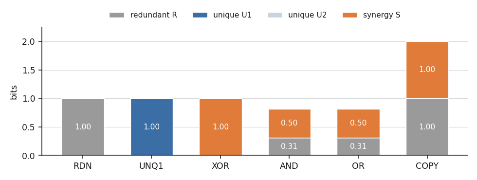
Stacked bars showing R, U1, U2 and S for the RDN, UNQ1, XOR, AND, OR and COPY gates

Fig. 1. The four atoms under I_min for six gates whose decomposition is known analytically. RDN is one bit of pure redundancy, UNQ1 one bit unique to the first source, XOR one bit of pure synergy. AND and OR carry both R and S at once. U2 is zero in all six by construction

Read the XOR column against the AND column. XOR is a full bit that lives nowhere except in the pair. AND is more typical of real data: either input alone raises your odds a little, 0.31 bits of redundancy, and the remaining half bit needs both. Real market pairs look like a much weaker AND.

The three measures this library carries

Because redundancy is an axiom rather than a derivation, competing definitions exist and they disagree. The library carries three of them, and lets the caller choose:

//+------------------------------------------------------------------+
//| Which extra axiom fixes the fourth unknown                       |
//+------------------------------------------------------------------+
enum ENUM_PID_MEASURE
  {
   PID_IMIN,      // Williams and Beer 2010, the original
   PID_IMMI,      // Barrett 2015, the smaller of the two mutual informations
   PID_ICCS       // Ince 2017, pointwise common change in surprisal
  };

I_min is the original Williams and Beer proposal: per target value, take the smaller of the two sources' specific information, then average. It guarantees non-negative atoms, which is why it is the default and the only measure the stacked indicator can display. I_MMI takes the smaller of the two mutual informations and always drives one unique atom to zero. I_ccs is Ince's pointwise measure, computed on a maximum-entropy distribution rather than on the data, and it can return negative atoms.

The COPY gate is where they part company. Two independent bits are copied into the target, so each source intuitively carries one bit the other does not. I_min answers R = 1 and S = 1, which says two independent coins are entirely redundant, the criticism that has followed the measure since 2010. I_ccs answers U1 = U2 = 1 with R = S = 0, and both come out of the same library on the same table:

[PID] [4] COPY - the axiom decides, and the two disagree
[PID]   PASS  I_min: R and S both one bit                      I_min R 1.000000 U1 0.000000 U2 0.000000 S 1.000000
[PID]   PASS  I_ccs: one bit unique to each source             I_ccs R 0.000000 U1 1.000000 U2 1.000000 S 0.000000

A whole bit of disagreement on a four-row table. The library asserts both readings rather than averaging them: the choice of axiom is a modeling decision the analyst makes, not a detail the code hides. Section 8 shows the same choice changing the verdict on real gold data.

The joint table, and the logarithms that are not in it

Everything above is defined on a joint probability distribution over three variables, and market data arrives as continuous doubles. So the first job is to turn (target, source, source) into a three-dimensional table of integer counts. That table is the only estimate the library makes; every entropy, every atom and every null draw is assembled from it.

The cost of the table is the product of the three bin counts. The shipped default is deliberately coarse, three bins for the target and five per source, 75 cells: 2435 rows of daily gold give about 32 rows per cell, while five target bins and seven source bins would give 10, at which point the atoms are mostly estimation bias. The facade prints that ratio next to every reading and says so in words below ten.

Equal-frequency bins, assigned by rank

Bins are equal-frequency, not equal-width. Equal-width bins on a fat-tailed return distribution put almost every row in the middle bin and leave the outer cells empty, and an empty cell contributes nothing while still costing sample-size budget.

//+------------------------------------------------------------------+
//| Equal-frequency bins, assigned by rank                           |
//|                                                                  |
//|  The rank comes from a stable order on (value, index), so equal  |
//|  values resolve the same way on both sides of the cross-check.   |
//|  Equal frequencies also keep every marginal near uniform, which  |
//|  is what leaves the joint table populated.                       |
//+------------------------------------------------------------------+
bool CPIDJoint::QuantileBins(const double &x[], const int n, const int nbins,
                             int &out[])
  {
   if(n <= 0 || nbins < 2)
      return(false);

//--- sort the positions rather than the values, so the original row of
//--- every observation survives the sort and can be written back to
   int idx[], work[];
   ArrayResize(idx, n);
   ArrayResize(work, n);
   for(int i = 0; i < n; i++)
      idx[i] = i;
   MergeIndex(x, idx, work, 0, n - 1);

//--- the bin is a share of the rank order, so it depends on nothing but
//--- position: a fat tail moves a value, never the bin it lands in
   ArrayResize(out, n);
   for(int rank = 0; rank < n; rank++)
     {
      int b = (int)(((long)rank * (long)nbins) / (long)n);
      if(b >= nbins)
         b = nbins - 1;   // the last bin absorbs the rounding
      out[idx[rank]] = b;
     }
   return(true);
  }

Sorting on (value, index) makes tie resolution deterministic. That allows the Python cross-check to demand exact equality rather than loose agreement. Ranking also means the split lands on the sample's own quantiles: fed a continuous exclusive-or planted at 0.5, the two-bin split lands on the median instead, and the recovered synergy rises from 0.717 bits at 3000 rows only to 0.908 at 48,000 rows. That shortfall is the binning, not the estimator.

Every logarithm looked up once

An entropy over a table of counts is a sum of terms of the form k*log2(k), and every k is an integer bounded by the number of rows. So no logarithm needs to be evaluated inside any loop:

//+------------------------------------------------------------------+
//| Tabulate every value the counts can take                         |
//|                                                                  |
//|  Index zero holds zero for both tables: an empty cell adds       |
//|  nothing to an entropy and must not reach MathLog.               |
//+------------------------------------------------------------------+
void CPIDLogTable::Build(const int maxCount)
  {
   int need = (maxCount < 1 ? 1 : maxCount) + 1;
   if(need <= m_size)
      return;   // a null reuses one table across thousands of decompositions

   ArrayResize(m_log2, need);
   ArrayResize(m_xlog2x, need);
   m_log2[0] = 0.0;
   m_xlog2x[0] = 0.0;
//--- every entropy in this library is built from integer cell counts, so
//--- tabulating the integers removes MathLog from every sweep that follows
   for(int k = 1; k < need; k++)
     {
      m_log2[k] = MathLog((double)k) * PID_LOG2E;
      m_xlog2x[k] = (double)k * m_log2[k];
     }
   m_size = need;
  }

Once the count table is built, each entropy reduces to log2(N) minus a lookup-based sum over cells. The permutation null rebuilds every entropy on every draw, so a 66-pair scan with 99 draws performs about 6500 full decompositions.

From redundancy to four atoms

With the table in hand, the lattice is arithmetic. Compute the three mutual informations, ask the chosen axiom for R, and the remaining three atoms fall out:

//+------------------------------------------------------------------+
//| Redundancy first, then the other three in closed form            |
//+------------------------------------------------------------------+
bool CPIDLattice::Decompose(const CPIDJoint &j, const CPIDLogTable &tab,
                            const ENUM_PID_MEASURE m, CPIDMaxEnt &fit,
                            SPIDAtoms &out)
  {
   out.Reset();
   out.measure = m;
   if(j.Total() <= 0)
      return(false);

//--- the three mutual informations are the only quantities Shannon fixes
   out.i1 = CPIDInfo::MutualTX1(j, tab);
   out.i2 = CPIDInfo::MutualTX2(j, tab);
   out.i12 = CPIDInfo::MutualTPair(j, tab);

//--- the axiom supplies the fourth, and the other three then subtract out
   out.r = CPIDRedundancy::Of(m, j, tab, fit);
   out.u1 = out.i1 - out.r;
   out.u2 = out.i2 - out.r;
   out.s = out.i12 - out.i1 - out.i2 + out.r;

//--- only I_ccs runs a fit, so only I_ccs can come back unreliable
   out.fitError = (m == PID_ICCS ? fit.Error() : 0.0);
   out.reliable = (m != PID_ICCS || fit.Converged());
   return(true);
  }

Two fields of the result say nothing about the market and exist so a caller cannot be fooled. fitError is how far the maximum-entropy fit behind I_ccs landed from its target marginals, and reliable is false when that fit did not converge, because a failed fit returns zero redundancy and zero redundancy is a plausible-looking decomposition.

Specific information, the term I_min averages

I_min is defined through a quantity most information-theory code never computes: the information a source carries about one particular value of the target, rather than about the target as a whole.

//+------------------------------------------------------------------+
//| I(t; X) for one target value, the term I_min averages            |
//|                                                                  |
//|  A relative entropy between p(x|t) and p(x), so it is never      |
//|  negative, and averaging it over t returns I(T;X).               |
//+------------------------------------------------------------------+
double CPIDInfo::SpecificInfo(const CPIDJoint &j, const CPIDLogTable &tab,
                              const int source, const int t)
  {
   int n = j.Total();
   int ct = j.CountT(t);
   if(n <= 0 || ct <= 0)
      return(0.0);

   int nx = (source == 1 ? j.N1() : j.N2());
   double sJoint = 0.0, sMarg = 0.0;
//--- accumulate the two halves of sum p(x|t) log( p(x|t) / p(x) ) in raw
//--- counts, so every logarithm is a table lookup on an integer
   for(int x = 0; x < nx; x++)
     {
      int ctx = (source == 1 ? j.CountT1(t, x) : j.CountT2(t, x));
      if(ctx <= 0)
         continue;   // an empty cell contributes nothing
      int cx = (source == 1 ? j.Count1(x) : j.Count2(x));
      sJoint += tab.XLog2X(ctx);
      sMarg += (double)ctx * tab.Log2(cx);
     }
//--- the trailing terms undo the count scaling the two sums carry
   return((sJoint - sMarg) / (double)ct - tab.Log2(ct) + tab.Log2(n));
  }

Averaging that quantity over t with weights p(t) returns exactly I(T;X), an identity the suite asserts over all six gates and which reproduces to 1.1e-16. Redundancy under I_min is the same average with the smaller of the two sources' terms taken at each t, which is where the name comes from.

The distribution behind I_ccs

I_ccs is not computed on the data. It is computed on the maximum-entropy distribution that reproduces the data's three pairwise marginals, the model with every pairwise interaction and no three-way term. The library reaches it by iterative proportional fitting: scale the table so its (T,X1) marginal matches the data's, then (T,X2), then (X1,X2), and repeat. On that distribution each cell contributes its local co-information, but only when all four local terms agree in sign, which is the "common change in surprisal" the measure asks for.

A fit that converges at 1/n, and the cell that has to go

The straightforward version of that fit does not work. On a deterministic table such as the AND gate the constraints force certain cells to zero, and proportional fitting approaches a zero only at rate 1/n: measured on AND, the worst marginal error is 8.065e-03 after 10 passes and 8.333e-06 after 10000, which is exactly 0.083/n. Reaching 1e-12 that way would need on the order of 1e11 passes.

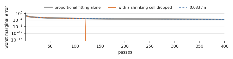
Log-scale plot of marginal error against passes, showing the 0.083 over n curve and a vertical drop to machine zero once a dying cell is dropped

Fig. 2. Proportional fitting alone tracks 0.083/n forever, in gray under the dashed reference. Dropping a cell that is still shrinking after a whole block of passes ends the fit at machine zero instead

The remedy has two parts, both needed. Cells whose row in any two-way marginal is zero are dropped before the first pass, since they cannot be anything else. Then, if the fit has still not converged after a block of passes, any cell that shrank measurably across that whole block is on its way to zero and is dropped too. The pruning round, excerpted from the middle of Fit:

//--- fit in blocks of passes, so a cell can be watched over an interval
   m_passes = 0;
   double before[];
   ArrayResize(before, cells);
   for(int round = 0; round < PID_IPF_ROUNDS; round++)
     {
      if(RunBlock())
         break;
      ArrayCopy(before, m_q);   // the state one block back
      if(RunBlock())
         break;

//--- a cell still shrinking across a whole block is on its way to zero,
//--- and the fit reaches that boundary only if the cell is dropped outright
      bool pruned = false;
      double kept = 0.0;
      for(int i = 0; i < cells; i++)
        {
         if(m_q[i] > PID_EPS && before[i] > PID_IPF_DECAY * m_q[i])
           {
            m_q[i] = 0.0;
            pruned = true;
           }
         kept += m_q[i];
        }
      if(!pruned || kept <= 0.0)
         break;
      for(int i = 0; i < cells; i++)
         m_q[i] /= kept;   // dropping mass costs a renormalization
     }

   m_error = MarginalError();
   return(Converged());
  }

A magnitude threshold cannot do this job: the dying cell in the AND gate still sits at 4e-04 after 200 passes, far above any epsilon you would call zero. It is the trend that identifies it, not its size. After the fix the fit reproduces every gate marginal to 0.000e+00, and market tables converge to about 1e-15 in 16 to 25 passes. I_ccs refuses to score a fit that did not get there.

The atoms do not read zero when nothing is there

This is the single most important property of the method, and every significance decision follows from it. Take two columns of independent uniform noise and an independent target, bin them into the shipped 3 x 5 x 5 grid, and decompose. There is nothing whatsoever to find. The library reports a positive number anyway:

[PID] [4] the finite-sample floor on independent columns
[PID]       rows   250   R 0.009956  S 0.100330  total 0.113182
[PID]       rows   500   R 0.004370  S 0.056004  total 0.066346
[PID]       rows  1500   R 0.006509  S 0.021054  total 0.032671
[PID]       rows  6000   R 0.000296  S 0.005197  total 0.005712

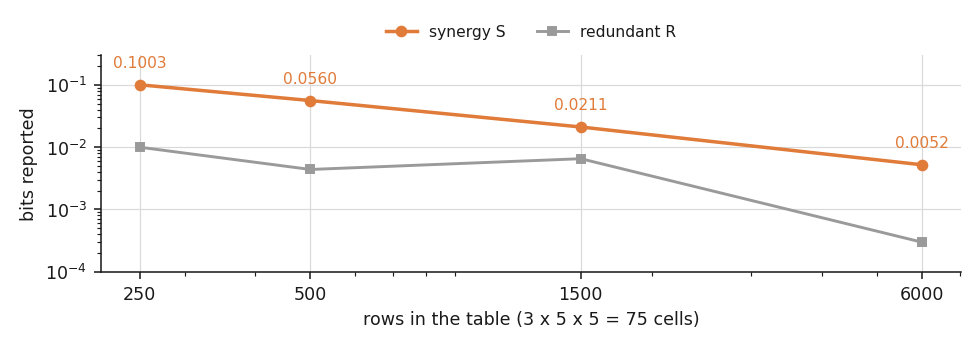
Log-log plot of reported synergy and redundancy against row count for independent columns, falling from 0.10 bits at 250 rows to 0.005 at 6000

Fig. 3. Synergy and redundancy reported on columns with no relationship at all. The floor falls as rows are added and never reaches zero, so no fixed threshold can stand in for it

The cause is straightforward: with 75 cells and 250 rows most cells hold two or three observations, and the accidental structure of that sparse table is indistinguishable from real structure. A raw atom cannot be interpreted, compared across settings, or thresholded. What can be is its position against a distribution built from the same data with the relationship destroyed: shuffle the target, keep the two sources paired exactly as they were, decompose again, and repeat.

The block length is load bearing

Shuffling one row at a time is the obvious implementation and it is wrong here, for the reason the function's own header states: a target that reads five bars forward makes neighboring rows share most of the same future bars, so the label sequence arrives in runs, and destroying them yields a null the data clears far too easily.

//+------------------------------------------------------------------+
//| Permute whole blocks, never single rows                          |
//|                                                                  |
//|  Rows a horizon apart share most of the same forward bars, so a  |
//|  label sequence arrives in runs. Shuffling one row at a time     |
//|  destroys those runs and yields a null the data clears too       |
//|  easily. A block of about twice the run length preserves them.   |
//+------------------------------------------------------------------+
void CPIDRandom::BlockShuffle(const int &src[], int &dst[], const int n,
                              const int block)
  {
   int b = (block < 1 ? 1 : block);
   int nblocks = (n + b - 1) / b;

//--- Fisher-Yates over the block order, so the blocks move and the rows
//--- inside each one never do
   int order[];
   ArrayResize(order, nblocks);
   for(int i = 0; i < nblocks; i++)
      order[i] = i;
   for(int i = nblocks - 1; i > 0; i--)
     {
      int j = Below(i + 1);
      int tmp = order[i];
      order[i] = order[j];
      order[j] = tmp;
     }

//--- write the blocks out in their new order; the last one is short
//--- whenever the block length does not divide the row count
   ArrayResize(dst, n);
   int w = 0;
   for(int k = 0; k < nblocks; k++)
     {
      int start = order[k] * b;
      int stop = MathMin(start + b, n);
      for(int i = start; i < stop; i++)
         dst[w++] = src[i];
     }
  }

The block length is settled by a false-positive sweep rather than asserted. Twenty pure random walks, twelve features each, all 66 pairs scored against a null of 39 draws at a nominal alpha of 0.05. Everything that fires here is false by construction:

[PID] [2] false positives on random walks, by block length
[PID]       nominal alpha 0.05, 20 walks, 39 draws
[PID]       block  1   per-pair 0.141   any pair fires 1.000   family-wise 0.700
[PID]       block  5   per-pair 0.065   any pair fires 1.000   family-wise 0.300
[PID]       block 10   per-pair 0.060   any pair fires 0.900   family-wise 0.250
[PID]       block 20   per-pair 0.070   any pair fires 1.000   family-wise 0.150
[PID]       block 40   per-pair 0.058   any pair fires 1.000   family-wise 0.150

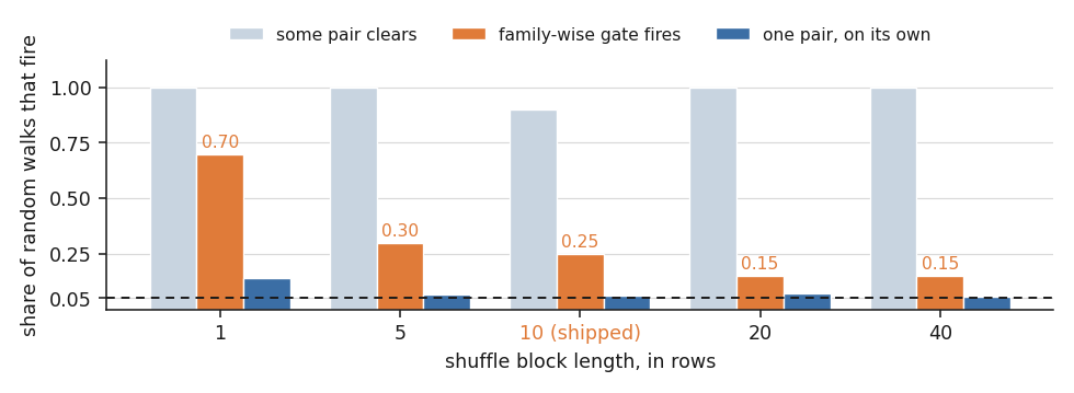
Grouped bars showing that some pair clears on nearly every walk, that the family-wise gate falls from 0.70 to 0.15 as the block grows, and that the per-pair rate stays near nominal

Fig. 4. False positives on twenty random walks. The dashed line is the nominal 0.05. An independent shuffle fires the family-wise gate on 70 percent of walks; blocks of twice the horizon bring it to 0.25

Two readings come out of that table. The per-pair rate is close to nominal at every block length but one, so a single pair tested on its own is roughly honest. The family-wise column, the middle bar of each group in Fig. 4, is where an independent shuffle does its damage: 70 percent of pure random walks at block 1, 25 percent at the shipped block of twice the horizon, 15 percent at blocks of 20 and 40. That column rules settings out rather than picking one, because a longer block also preserves more of the sequence and so makes the null harder for a real effect to beat, a cost nothing here measures. Note too that the middle bar never reaches the dashed 0.05: the honest figure for a twelve-feature search is 0.25 at the shipped setting and 0.15 at best.

The p-value floor, which can make significance unattainable at a given alpha

A permutation p-value cannot be smaller than one over the number of draws plus one, and for a two-sided test it cannot be smaller than twice that:

//+------------------------------------------------------------------+
//| A two-sided p-value, with ties counted as at least as extreme    |
//|                                                                  |
//|  Counting ties on both sides is the standard permutation-test    |
//|  treatment and errs toward refusing rather than reporting.       |
//+------------------------------------------------------------------+
double CPIDNull::PValue(const int atom, const double observed)
  {
   if(m_draws <= 0)
      return(1.0);
//--- count both tails, since an atom can be surprising by sitting below
//--- its null as well as above it
   int ge = 0, le = 0;
   for(int k = 0; k < m_draws; k++)
     {
      double v = m_draw[k][atom];
      if(v >= observed - PID_EPS)
         ge++;
      if(v <= observed + PID_EPS)
         le++;
     }
//--- the observation counts as its own draw, which is what puts the
//--- floor at 2/(draws+1) rather than at zero
   double up = (double)(ge + 1) / (double)(m_draws + 1);
   double lo = (double)(le + 1) / (double)(m_draws + 1);
   return(MathMin(1.0, 2.0 * MathMin(up, lo)));
  }

//+------------------------------------------------------------------+
//| The smallest p-value the draw count can produce                  |
//|                                                                  |
//|  A two-sided p is twice the one-sided tail, so the floor is      |
//|  2/(ndraw+1). Ask for a threshold below it and no result can     |
//|  ever clear, however strong the effect.                          |
//+------------------------------------------------------------------+
double CPIDNull::PFloor(const int ndraw, const bool twoSided = true)
  {
   if(ndraw <= 0)
      return(1.0);
   return((twoSided ? 2.0 : 1.0) / (double)(ndraw + 1));
  }

The edge is easy to walk into. With 19 draws the smallest two-sided p is 0.10, so a gate at alpha = 0.05 can never fire however strong the relationship, and such a scan reports zero significant pairs on every dataset. The library states its own floor beside every reading. The tie rule in the same block matters for a statistic the shuffle nearly preserves: without it the comparison turns on the last bit or two of a number carrying no information.

Important: the two-sided floor is 2/(draws+1), not 1/(draws+1). The default of 39 draws gives exactly 0.05, so the shipped indicator can just reach a 0.05 gate and no lower. Asking for alpha = 0.01 needs at least 199 draws.

Scanning every pair, and paying for the null once

Fig. 4 already priced the search itself: on pure noise, some pair among the 66 clears its own gate on 90 to 100 percent of random walks, so the winner has to be compared against the distribution of winners. What makes that affordable is that one shuffled target is scored against every pair before the next shuffle is drawn, excerpted here from ScanPairs:

   CPIDRandom rng;
   rng.Seed(m_seed);
   int shuffled[];
   SPIDAtoms a;

//--- one shuffle per draw, scored against every pair: that yields the
//--- per-pair nulls and the distribution of the winner for the same cost
   for(int k = 0; k < m_draws; k++)
     {
      rng.BlockShuffle(tbin, shuffled, rows, m_block);   // blocks keep the target's runs
      double best = -1.0e308;
      for(int p = 0; p < m_npairs; p++)
        {
         for(int i = 0; i < rows; i++)
           {
            ba[i] = bins1[c1[p] * rows + i];
            bb[i] = bins2[c2[p] * rows + i];
           }
         if(!j.Build(shuffled, ba, bb, rows, m_nt, m_n1, m_n2))
            return(false);
         if(!CPIDLattice::Decompose(j, m_tab, m_measure, fit, a))
            return(false);
         m_drawS[k * m_npairs + p] = a.s;
         drawR[k * m_npairs + p] = a.r;
         if(a.s > best)
            best = a.s;
        }
      m_familyBest[k] = best;   // the best-of-all-pairs this draw reached
     }

Each draw yields 66 decompositions, exactly what the per-pair nulls cost anyway; the extra product is the maximum over pairs, recorded in m_familyBest, so the family-wise p-value is free.

Verification: analytic gates, an outside reference, one shared stream

The library is verified at three levels, and they are deliberately different in kind.

The gates need no reference at all. XOR, AND, OR, COPY, RDN and UNQ1 have decompositions that can be worked out on paper, so a test that reproduces them is checking against mathematics rather than against another implementation:

[PID] [1] XOR - neither source alone carries anything
[PID]   PASS  I(T;X1) is zero                                  0.000000000
[PID]   PASS  I(T;X2) is zero                                  0.000000000
[PID]   PASS  I(T;X1,X2) is one bit                            1.000000000
[PID]   PASS  S is one bit                                     1.000000000

The Python reference is real and independent. dit 2.2 installs and runs on the current Python, and it implements the same three measures as PID_WB, PID_MMI and PID_CCS. The cross-check rebuilds every exported table from its own labels, decomposes it with the blueprint, and compares against both the MQL5 export and dit.

The random stream is shared, so the null is an equality rather than a comparison. MQL5's ulong and Python's masked integers wrap identically, so splitmix64 seeding xorshift64* produces the same 64-bit words on both sides. The permutations are not statistically similar to the MQL5 ones; they are the same permutations, and the two nulls have to agree draw for draw:

[6] the null, redrawn from the same stream
  PASS  39 draws reproduce exactly                           worst 4.460e-15
  PASS  the p-value for S is well formed                     p 0.2000, floor 0.0500
  PASS  the null mean for S sits above zero                  0.013087 against an observed 0.017743
23 PASS, 0 FAIL   [ALL PASS]

The full status of the chain, as measured on 2026.08.25:

Level	Script or command	Result
Blueprint	python pid_prototype.py	29 PASS, 0 FAIL
Stream and table	PID_Test_Info.mq5	24 PASS, 0 FAIL (9 ms)
Analytic gates	PID_Test_Gates.mq5	23 PASS, 0 FAIL (1.9 ms)
Lattice on data	PID_Test_Lattice.mq5	26 PASS, 0 FAIL (0.08 s)
Null and search	PID_Test_Null.mq5	10 PASS, 0 FAIL (2.4 s)
Cross-check	export, then python pid_crosscheck.py	23 PASS, 0 FAIL
Market	PID_Scan_Market.mq5	XAUUSDm D1, 2435 rows, 155 to 170 ms per scan

Run the export before the cross-check; the Python side reads the file the MQL5 script writes, and a stale export fails the assertions by design. Point PID_EXPORT at it if it lands elsewhere. One band above is asymmetric on purpose: I_ccs agrees with dit to 6.137e-11 where I_min and I_MMI agree to about 4e-15, because dit reaches the same distribution through a general optimizer whose own residual is around 1e-10. The looser band is not our error.

What gold actually says

The data layer turns bars into twelve causal features and one of three forward targets. Every feature is computed only from bars at or before its own row, and every target reads forward, so a row stops existing a horizon short of the newest bar.

#	Feature	What it is	#	Feature	What it is
0	ret1	log return over 1 bar	6	bbPos	position inside the Bollinger band
1	ret5	log return over 5 bars	7	atrRatio	ATR(14) over ATR(50)
2	rsi14	Wilder RSI	8	maDist	distance from SMA(20) in ATR
3	stoch14	stochastic position in the 14-bar range	9	volZ	tick volume z-score over 50 bars
4	cci20	commodity channel index	10	rangeATR	bar range in ATR
5	macdHist	MACD histogram scaled by ATR	11	streak	signed run length of same-direction bars

The index in that table is what InpFeature1 and InpFeature2 take in the indicator and in the expert; both ship set to 0 and 9, ret1 and volZ. The three targets are the signed forward return, its absolute value, and forward realized volatility. Which one you ask about changes the answer completely.

Three targets against two controls

A control only refutes a finding when it answers the same question, so each target is scored three ways in one pass: on the real bars, on the same bars reordered in time, and on a random walk matched to the real series in drift and spread. The reordering is the sharper of the two, since every bar keeps its own return, its wicks and its volume and only the sequence is destroyed.

[PID] [2] three targets against two controls
[PID]       target            source        cleared  best S   pFam
[PID]       fwd return        real          7 of 66  0.02917  0.0700
[PID]       fwd return        shuffled      5 of 66  0.02496  0.1800
[PID]       fwd return        walk          1 of 66  0.02329  0.1100
[PID]       |fwd return|      real          9 of 66  0.02538  0.0900
[PID]       |fwd return|      shuffled      2 of 66  0.02220  0.2100
[PID]       |fwd return|      walk          8 of 66  0.02073  0.1700
[PID]       fwd volatility    real         11 of 66  0.04094  0.0100
[PID]       fwd volatility    shuffled      6 of 66  0.03629  0.0100
[PID]       fwd volatility    walk          3 of 66  0.02541  0.0600

The last two columns answer different questions. cleared counts the pairs whose own S beat their own null, 66 separate tests; pFam asks how often the best of all 66 pairs, on a shuffled target, reaches what the best real pair reached, so a row can clear more pairs and carry the worse family-wise p. On the signed return the real bars clear 7 of 66 against the shuffled control's 5 and read pFam 0.0700, which does not clear alpha at all: nothing there, the same conclusion a completely different method reached on this instrument.

Forward volatility stands furthest from both controls, and the cleared column is not what says so: there the signed return looks stronger, and it is the target just called empty. The separation is in the family-wise p, 0.0100 against the walk's 0.0600. The shuffled row also reads 0.0100, but that value is the 99-draw floor. The meaningful separation is in Fig. 5: the best real pair scores 0.04094 bits against 0.03629 after time reordering. A real gap, and a small one.

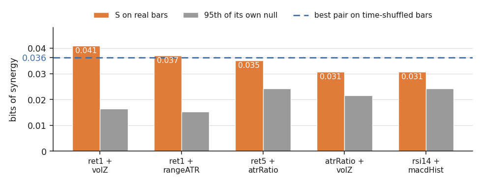
Bars comparing synergy on real bars against the 95th percentile of each pair's own null, with a dashed line marking the best pair found on time shuffled bars

Fig. 5. The five strongest pairs on forward volatility, each against the 95th percentile of its own null. The dashed line is the best pair the same scan finds after the bars are reordered in time, which lands above three of the five real pairs

Important: one scan is one draw. Running the identical scan one day later, so the 2500-bar window slides by a single bar, moved the shuffled control's family-wise p from 0.0700 to 0.0100 while the real row barely moved. Run the table over several end dates before treating any of it as a property of gold.

The same bars under all three axioms

Section 3 argued that the choice of redundancy measure is a modeling decision. Here is that decision changing the verdict on real data: same bars, same bins, same null, on both of the targets above:

Target	Axiom	Pairs clearing alpha	Best pair	Best S	Family-wise p
fwd volatility	I_min	11 of 66	ret1 + volZ	0.04094	0.0100
fwd volatility	I_MMI	13 of 66	ret1 + volZ	0.04167	0.0100
fwd volatility	I_ccs	21 of 66	ret1 + rangeATR	0.03597	0.0100
signed return	I_min	7 of 66	rsi14 + macdHist	0.02917	0.0700
signed return	I_MMI	7 of 66	rsi14 + macdHist	0.03042	0.0500
signed return	I_ccs	4 of 66	rsi14 + atrRatio	0.02356	0.3200

Read the two blocks against each other, because either alone would mislead. On forward volatility, I_ccs clears 21 of 66 pairs where I_min clears 11, and the two disagree on which pair is strongest. On the signed return the ordering reverses: I_ccs becomes the most conservative at a family-wise p of 0.3200, while I_MMI lands exactly on a gate of alpha 0.05, on the same bars where I_min missed at 0.0700. The direction verdict above is therefore a statement about I_min, not about gold. Report the axiom alongside the atom, always.

Does the reading survive out of sample

The scan splits the history at 70 percent, ranks the pairs on the head, and asks what the tail says about them. The tail holds 685 rows against the head's 1685, and by Fig. 3 the floor rises as rows fall, so the raw out-of-sample atom is not comparable. Rank among the 66 and distance from the tail's own null are:

[PID] [4] out-of-sample transfer of the chosen pairs
[PID]       head 1685 rows, tail 685 rows - the floor differs, so rank is the comparable column
[PID]       pair                   rank in  rank out   over null95
[PID]       atrRatio + volZ              1        18           no
[PID]       rsi14 + atrRatio             2         1           no
[PID]       mean out-of-sample rank 23.2 of 66, chance would give 33.5
[PID]       1 of 5 clear their own out-of-sample null

The five strongest in-sample pairs land at a mean out-of-sample rank of 23.2 of 66 against the 33.5 chance would give. The ordering carries a little, and not much: one of the five clears its own out-of-sample null, and the head's strongest pair falls to rank 18.

Put the three results together and the summary is short. The direction target carries nothing that survives its own control under the default axiom, and only touches the gate under the most permissive of the three. The volatility target carries a little more than a matched random walk, its advantage over reordered bars is small, its family-wise p is pinned to the resolution floor, and its ranking only partly survives a purged split.

Consuming the reading

The indicator

A decomposition is four numbers that sum to a fifth, so the natural display is a stack rather than a line. The indicator draws R, then R+U1, then R+U1+U2, then the total, as four histograms in a subwindow, so each atom is the band between two adjacent bars. Over the top it draws one dotted line: the same total with S replaced by the 95th percentile of that window's own null. Excerpted from the plotting loop:

//--- a decomposition costs tens of milliseconds, so only every step-th bar
//--- recomputes and the bars between it hold the reading that came before
   for(int bar = firstBar; bar < rates_total; bar++)
     {
      bool due = (((bar - firstBar) % InpStep) == 0);
      if(due)
        {
         SPIDAtoms tmp;
         double tn = 0.0, tp = 1.0;
         int tr = 0;
         if(ReadAt(bar, tmp, tn, tp, tr))
           {
            a = tmp;
            n95 = tn;
            pv = tp;
            rows = tr;
            have = true;
            computed++;
           }
        }
      //--- nothing is drawn until the first window succeeds, so the line
      //--- never opens on a reading that was never computed
      if(!have)
         continue;

//--- cumulative sums, so the four atoms render as one stack; the null rides
//--- on the same base as S, and the stack top crossing it is the reading
      g_r[bar] = a.r;
      g_ru1[bar] = a.r + a.u1;
      g_ru1u2[bar] = a.r + a.u1 + a.u2;
      g_total[bar] = a.r + a.u1 + a.u2 + a.s;
      g_noise[bar] = a.r + a.u1 + a.u2 + n95;
      g_s[bar] = a.s;
      g_p[bar] = pv;
      g_null95[bar] = n95;
     }

That geometry is the whole point of the display. The top band rising above the dotted line is what "synergy clears its null" looks like, with no second axis to read and no mental comparison between two plots.

Three properties matter before attaching it. The line is a staircase, computed every InpStep bars and held in between, because each reading costs a permutation null. The window ends at the newest closed bar. And InpWindow asks for 600 rows against the scan's 2435, so by Fig. 3 the dotted line sits several times higher here, which is why the null is redrawn per window rather than fixed once.

Cost, measured from inside the indicator with GetMicrosecondCount: 25 to 50 ms for 40 windows over 200 plotted bars, across six loads on an idle terminal, so InpHistoryBars can be generous. Fig. 6 is not one of those loads; a screenshot shares the chart thread, and that run reported 41 ms in the panel and 53 ms in its log for the same work.

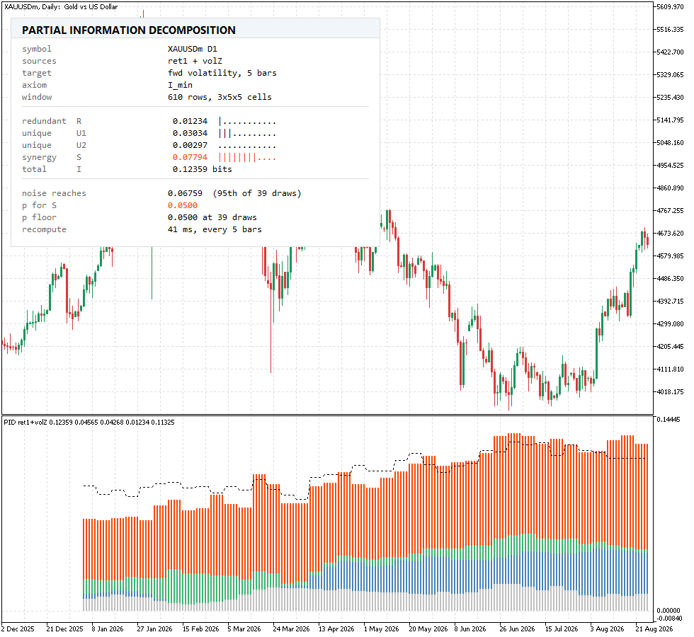
Subwindow showing the four atoms stacked with the null level drawn over the stack, and a panel listing the atoms, the level noise reaches, the p-value and the floor that p-value can reach

Fig. 6. The four atoms stacked in the subwindow, with the dotted line marking the level noise reaches. The panel reports the same reading numerically, including the p-value and the resolution floor the draw count allows

That reading clears by the narrowest margin the display can report: synergy 0.07794 against a level noise reaches of 0.06759, with the p-value at 0.0500 sitting exactly on the floor 39 draws allow. One draw landing above the observation would have made it a miss with the picture unchanged. Note too that null95 is one-sided while the p doubles the tail, so a band clear of the line that still misses the gate is an ordinary state here. The answer to both is more draws.

The expert, and the control that beat it

The decomposition produces a strength and never a direction, so it cannot be an entry signal. What it can do is decide whether a joint reading of two features is worth trusting, and the expert uses it for exactly one job: sizing the stop. The entry is a plain Donchian breakout in every arm, and only the volatility number the stop is built from differs between them.

//+------------------------------------------------------------------+
//| The volatility this bar's stop is built from                     |
//|                                                                  |
//|  All three arms take the same entry and the same formula, so     |
//|  only this number differs between them. When the decomposition   |
//|  is not significant every arm falls back to the sample mean, so  |
//|  the three trade populations stay close without being equal.     |
//+------------------------------------------------------------------+
double VolatilityNow(const double v1, const double v2)
  {
//--- the control arm, and the fallback for every arm when the pair's
//--- synergy did not clear its own null
   double global = g_rule.GlobalMean();
   if(!g_significant || InpVolMode == PID_VOL_CONSTANT)
      return(global);

//--- the reading itself: the mean of the joint cell this bar lands in
   double cell = g_rule.PredictAt(v1, v2);
   if(InpVolMode == PID_VOL_INVERTED)
      cell = 2.0 * global - cell;   // the opposite control, reflected about the mean
//--- a thin cell can hold an extreme mean, so clamp before it sizes a stop
   if(cell < global * 0.20)
      cell = global * 0.20;
   if(cell > global * 5.00)
      cell = global * 5.00;
   return(cell);
  }

Three arms share that function. Constant always uses the sample mean, the control for "the decomposition contributes nothing". Cell uses the average of the target inside the joint cell the live pair falls into, which is the reading. Inverted mirrors that cell estimate through the sample mean, the control for "the reading is actively wrong". The last column is the standard deviation of the per-trade stop distance as a percentage of its own mean.

Arm	Trades	Net	Profit factor	Per trade	Balance drawdown	Stop spread
Constant (control)	142	+347.03	1.01	+2.44	9.80%	55.6%
Cell (the reading)	143	+512.30	1.01	+3.58	9.95%	56.7%
Inverted (control)	142	+731.14	1.01	+5.15	9.46%	55.0%

XAUUSDm D1, 2018.01.01 to 2026.08.01, 100000 deposit, 1 percent risk per trade, pair ret1 + volZ against forward volatility. The inverted control is the best arm on net profit, on per-trade expectancy and on drawdown, which is the ordering a working forecast never produces. All three are flat anyway: profit factor 1.01 in every arm and a spread of 0.35 to 0.73 percent over eight and a half years.

The chain behind that result is more interesting than the table. The grid is not flat, so the forecast had room and the clamp never bit. What kills it is the gate: eleven or twelve of sixteen retrains found no significant synergy, so most trades ran the identical constant in all three arms and the stop spread rises only from 55.6 to 56.7 percent between the control and the reading. Range in the grid, a gate that rarely opens, and 142 trades that cannot separate the arms.

Important: the expert is a demonstration of how the reading can be consumed, and no edge is claimed. It is included because the three-arm control is the honest way to test a forecast, and because the arm that was supposed to be wrong won. A backtest of the cell arm alone, with no controls beside it, would have looked like a small success.

Conclusion

The library does what it set out to do. It splits the information two indicators carry about a target into unique, redundant and synergistic parts; it carries three competing definitions of redundancy and shows them disagreeing by a whole bit on a four-row table; it verifies the arithmetic against analytic gates, an independent Python reference and a permutation null that is bit-identical across both languages; and it scans all 66 pairs in about 160 milliseconds with the family-wise correction included.

What it does not do is find an exploitable edge on gold, and what lets it say so with confidence is the discipline around the number rather than the number itself. Three things carried the argument: the floor measured on independent columns, which proves a raw atom means nothing; the block permutation null, whose length is defended by a false-positive sweep rather than asserted; and the two controls scored on the same target as the finding they refute. Take any one away and the volatility result reads like a discovery.

What ships with the article: eleven header files carrying the joint table, the entropies, three redundancy axioms, the lattice, the block-permutation null, a causal feature layer and a grid-based forecast rule; four test scripts; an export script paired with a Python cross-check that verifies the atoms against dit and the null draw for draw; a market scan; an indicator; and an expert. The table below lists them individually.

#	Filename	Type	Description
1	PID.mqh	Include	The facade: every pair, the family-wise null, the winner
2	PIDJoint.mqh	Include	Equal-frequency binning and the three-way count table
3	PIDLogTable.mqh	Include	log2(k) and k*log2(k) tabulated once, so no sweep calls MathLog
4	PIDInfo.mqh	Include	Entropies, mutual and specific information, from counts
5	PIDRedundancy.mqh	Include	The axiom: I_min, I_MMI, I_ccs and the maximum-entropy fit
6	PIDLattice.mqh	Include	Redundancy in, four atoms out, consistency equations exposed
7	PIDRandom.mqh	Include	splitmix64 into xorshift64*, and the block shuffle
8	PIDNull.mqh	Include	The permutation null, its percentiles and its p-value floor
9	PIDData.mqh	Include	Bars into twelve causal features and three forward targets
10	PIDRule.mqh	Include	The joint grid read as a forecast, bin edges kept
11	PIDPanel.mqh	Include	Panel geometry, shared by the display and the check on it
12	PID_Test_Info.mq5	Script	Stream conformance, the lookup table, mutual information twice
13	PID_Test_Gates.mq5	Script	The six gates against their analytic decompositions
14	PID_Test_Lattice.mq5	Script	Identities, planted relationships, the floor and the cost
15	PID_Test_Null.mq5	Script	False positives by block length, and power
16	PID_Export_ForCrosscheck.mq5	Script	The pipeline at full precision, for the Python side
17	PID_Scan_Market.mq5	Script	Real bars, both controls, three targets, axioms, transfer
18	PID_Synergy.mq5	Indicator	The four atoms stacked under the level noise reaches
19	PID_Volatility_EA.mq5	Expert	A demonstration: a stop from the joint cell, two controls
20	pid_prototype.py	Python	The blueprint and its oracles, checked against dit
21	pid_crosscheck.py	Python	The export against dit, against numpy and against itself
22	MQL5.zip	Archive	All project files in their subfolders; unpack into the terminal data directory

Attached files |

Download ZIP

MQL5.zip (72.79 KB)

Warning: All rights to these materials are reserved by MetaQuotes Ltd. Copying or reprinting of these materials in whole or in part is prohibited.

This article was written by a user of the site and reflects their personal views. MetaQuotes Ltd is not responsible for the accuracy of the information presented, nor for any consequences resulting from the use of the solutions, strategies or recommendations described.