Uncertainty as a Model (Part 4): Random Processes — The Dynamics of Uncertainty

Table of Contents

1. Foreword
2. Introduction
3. Definitions and Terminology
1. Definition of a Random Process
2. Cross-Sections and Sample Paths
3. Finite-Dimensional Distributions
4. Main Characteristics
4. Classification of Processes
1. By Time Structure
2. By State-Space Structure
3. Stationary Processes
4. Processes with Stationary Increments
5. Processes with Independent/Uncorrelated Increments
6. Ergodic Processes
7. Markov Processes
8. Martingales
5. Key Approaches
1. Linear Theory
2. Nonlinear Theory
3. Econometrics
4. Itô Calculus
6. Examples of Random Processes
1. Discrete White Noise
2. Discrete Random Walk
3. Wiener Process
4. Poisson Process
5. Markov Chain
7. Conclusion
8. Appendix
9. List of Attached Files

Foreword

We began by studying a single random variable, then moved on to collections consisting of a fixed number of variables. In examining limit theorems — the law of large numbers (LLN) and the central limit theorem (CLT) — we saw that such a collection can contain an arbitrarily large number of elements.

Now it is time for a key step: extending the concept of a collection of random variables to infinitely many variables. This will lead us to the concept of a random process.

Introduction

We look at a price or equity chart and have to make decisions based on a single sample path: where is the structure, and where is the random noise? Without a clear understanding of the language of random processes, discussions of stationarity, increments, Markov regimes, and martingales often devolve into a string of “smart-sounding words,” and backtesting becomes a questionable form of extrapolation. This article serves as a roadmap: by taking any time series (price, returns, increments, equity, order flow), we will learn how to correctly identify the object, pinpoint its key characteristics, and understand which class of processes it most closely resembles. In practice, this will allow us to formulate testable hypotheses and select appropriate analytical tools, rather than forcing the model to fit visual patterns.

Definitions and Terminology

Definition of a Random Process

Mathematically, a random process is a natural generalization of a set of random variables. Previously, we considered them as functions of a single argument ω from the probability space Ω: X₁(ω), X₂(ω), ..., Xₙ(ω). This sequence can easily be represented as a single function of two arguments: X(ω, i), where the index i belongs to the set I = {1, 2, ..., n}.

Further generalization removes restrictions on the index set I (index set). For trading, the most important cases are those in which I can be interpreted as time — that is, a fully ordered set. In this interpretation, the index set is denoted by T, and its elements by t. Usually, T is a subset of the real numbers.

Thus, by definition, a random process is a function X(ω, t) that assigns a specific numerical value to each pair consisting of ω and t (an event and a time).

Another generalization is also possible. The set of values that a random process X(ω, t) can take is called the state space. In advanced theory, it can be of any kind: vector-valued, complex-valued, complex vector-valued, or even more abstract. This flexibility in defining time and the state space makes it possible to create a vast variety of models. However, in this article, we will limit ourselves to the sets of real and natural numbers. This framework is sufficient to describe most market phenomena.

Cross-Sections and Sample Paths

To get the full picture, let’s introduce two key concepts that allow us to view the process from different angles:

1. Cross-section of the process. If we fix the time t = t₀, we obtain an ordinary random variable X₀(ω) = X(ω, t₀). This is the state of the system at a particular selected point in time.
2. Realization (or trajectory). If we fix an elementary event ω = ω₀, we obtain an ordinary numerical function of time: x₀(t) = X(ω₀, t).

For a trader, the trajectory is precisely the historical quote chart we see in the trading terminal. This leads to an important interpretation: a random process can be understood as a random function. Each event ω corresponds to its own unique curve — whether it is a price chart or the equity curve of a trading robot.

Finite-dimensional distributions

In essence, a random process is an infinite collection of random variables. However, probability theory does not provide a direct framework for working with infinite-dimensional distributions. To get around this limitation, mathematicians rely on the theory already developed for finite collections.

Definition: The finite-dimensional distribution of a random process X(ω, t) for given time points t₁, t₂, ..., tₙ is the joint distribution of its cross-sections at these time points: X(ω, t₁), X(ω, t₂), ..., X(ω, tₙ).

In this theory, it is generally assumed that we know all finite-dimensional distributions of the process. This makes it easy to determine the characteristics of quantities expressed in terms of a finite number of cross-sections. A typical example for a trader is the price increment between times t₁ and t₂. The problem of finding its distribution and characteristics is solved entirely through the joint distribution of the two corresponding cross-sections.

The real difficulties begin when the quantity of interest depends on an infinite number of points. For example, suppose we need to find the probability that, over a given time interval, the price will not touch the stop-loss level even once; formally, this is a problem involving the maximum or minimum of a process in continuous time. Problems like these require a much more sophisticated mathematical framework. Furthermore, such problems cannot be solved for random processes “in general.” Answers can be found only for particular types of such processes, which leads us to the need to distinguish separate classes of random processes.

Key Characteristics (Moments) of Random Processes

Based on finite-dimensional distributions, we can calculate the key characteristics of the process. It is important to understand that, unlike a typical random variable, the output here consists not of numbers but of (ordinary, non-random) functions of time:

1. The expected value of a process. It is calculated using one-dimensional distributions for each time t. If it exists, then it is a function of time, M(t).
2. Process variance. Similarly, this is calculated using one-dimensional distributions for each time t. This is the function D(t), which describes how the spread of the process changes over time.
3. The covariance function of a process. It is calculated using two-dimensional distributions for any pair of time points t₁ and t₂. This is a two-argument function, Cov(t₁, t₂), which shows the statistical relationship between the states of a process at different times. The covariance function of a random process is often referred to as the autocovariance function or simply autocovariance. The prefix “auto” emphasizes that we are looking for a relationship between the process and not some external series, but the process itself taken at different points in time.
4. Correlation function of the process. It is obtained by the usual normalization of covariance by the square root of the product of the variances: Corr(t₁, t₂) = Cov(t₁, t₂) / sqrt(D(t₁) * D(t₂)). It helps us understand to what extent a random process “remembers” its past states. In the literature and in statistical software packages, this function is often referred to as the autocorrelation function or autocorrelation (abbreviated as ACF). This underscores the fact that we are measuring the process's relationship to itself, but with a certain time lag.

Classification of Processes

It is important to understand that random processes are such complex objects that there is no single "comprehensive" classification. There is no table into which any arbitrary process could be entered. In practice, the classification identifies several distinct classes (subsets) for which mathematicians have made progress in solving practically important problems. It is precisely within these "islands of predictability" that most models are built.

By time structure

The type of time determines exactly how we record the data:

1. Discrete time. Points in time form a sequence. For example, the closing prices of H1 bars. In this case, the process itself is often referred to as a random sequence, while one specific realization is called a time series.
2. Continuous time. When we consider the process at any arbitrary instant. For example, a theoretical model of price movement in which ticks can arrive at any moment. Here, a process is interpreted as a random function, and its realization is simply referred to as a function or a trajectory.

By state-space structure

The type of state space determines the data being recorded:

1. Discrete state space. The process takes values from a countable set (for example, integers). In trading, this could be the number of open orders, the number of ticks in a bar, or the number of the current trading session.
2. Continuous state space. A process can take on any value within a specified interval (or the entire real number line). The most obvious example is the price of an asset or the value of a technical indicator (RSI, Moving Average).

It is important to understand that the classifications by time and by state are independent of one another. In practice, all four combinations are possible.

Stationary processes

In theory, there are two levels of "strictness" in the requirements for process stability:

1. Strict stationarity. This is maximum stability. Any finite-dimensional distributions at times (t₁, t₂, ..., tₙ) must coincide exactly with the distributions at times (t₁ + t, t₂ + t, ..., tₙ + t) for any shift t. Simply put: the probabilistic properties of the market in this model remain completely unchanged when shifted in time.
2. Wide-sense stationarity. The requirements here are much less stringent, which makes this class of processes the primary working tool in econometrics. Wide-sense stationarity requires only three conditions:
1. The expected value M(t) does not change over time (it is constant).
2. The variance D(t) is independent of time (a constant).
3. The covariance Cov(t₁, t₂) remains unchanged when the time points are shifted by the same amount: Cov(t₁, t₂) = Cov(t₁ + t, t₂ + t).

The last condition is critically important: it means that the relationship between two points in the process depends not on when we selected them, but solely on the distance (lag) between them. In other words, the covariance becomes a function of a single argument: Cov(t₁, t₂) = Cov(t₁ - t₂) = Cov(τ), where τ = t₁ - t₂. It is precisely this property that forms the basis for the analysis of autocorrelation functions.

Clarification on terminology: nonstationary processes are all processes that do not meet the definition of stationary processes. This is often a source of confusion for those who are familiar with stochastic processes only from a simplified econometrics course. In that context, the concept of nonstationarity is sometimes mistakenly narrowed down to specific cases — for example, the presence of a "unit root" or an explicit linear trend in autoregressive models. In fact, the world of nonstationary processes is much richer: it includes processes with varying volatility (heteroscedasticity), structures with changing memory, and, in general, any systems whose statistical properties “drift” over time. If even one condition for stationarity is violated, the process is formally considered nonstationary.

Processes with Stationary Increments

The increment of a process is a random variable equal to the difference between its cross-sections at two different points in time. By analogy with the stationarity of the processes themselves, the stationarity of increments is also divided into two forms:

1. Strict-sense stationarity. Any set of increments retains its joint distribution when shifted in time. The main condition is that the relative positions of all the points defining these increments must remain unchanged.
2. Wide-sense stationarity. The requirements here are less strict:
1. The expected value and variance of a single increment depend only on the length of the time interval between its start and end;
2. The covariance (and correlation) between two different increments remains unchanged under any time shift, provided that their lengths and the temporal distance between them remain constant.

Processes with Independent/Uncorrelated Increments

For a process with independent increments, any finite set of its increments, taken on disjoint time intervals, constitutes a collection of independent random variables. To avoid confusing them with processes with stationary increments, it is important to note a fundamental difference:

• By definition, any stationary process has stationary increments.
• However, a stationary process can have independent increments only in one degenerate case — if it is identically constant. This can be explained by the fact that, in a stationary process, the values at different points in time are "anchored" to a common mean, which inevitably creates dependence between the increments.

It is also worth remembering the hierarchy: any process with independent increments is a Markov process (since knowing the current state is sufficient to predict the next step). However, the converse is not true: there are many Markov processes whose increments are dependent.

Processes with uncorrelated increments are a weaker form (analogous to wide-sense stationarity), in which independence is replaced by the absence of a linear relationship. By definition, in such processes, any pair of increments on non-overlapping time intervals has zero correlation. An important difference from processes with independent increments:

• for independence, we needed the condition to hold jointly for any set of increments,
• for uncorrelatedness, it is sufficient that the condition hold pairwise.

Ergodic Processes

Ergodicity is a property that allows the characteristics of a process to be estimated from its sample paths. If only a single sample path of a general process is available, it is impossible to estimate its true expected value even approximately: this would require many independent realizations. However, if the process is ergodic, the average value over a single long sample path becomes a reliable approximation of the expected value of the entire process. In this sense, ergodicity is very similar to the Law of Large Numbers (LLN) from classical probability theory.

Ergodicity is typically defined for strictly stationary processes. However, due to its immense practical importance, this concept is often extended to broader classes of quasi-stationary processes. In addition to full ergodicity, “partial” ergodicity is often considered sufficient: a process may be ergodic with respect to its expected value but not with respect to its variance.

For a trader, ergodicity is a "license" to use backtests. If the market is ergodic to some extent, we can trust that the patterns identified in historical data reflect the general nature of the asset, rather than being a mere coincidence over a specific time period.

Markov Processes

These are processes with “short memory”: their future state depends only on the present and is in no way influenced by the past. Mathematically, this means that if we know the current value, knowing the entire history up to that point will not give us any additional information about the likely movement in the moments that follow. The conditional distribution for a future value of a process is determined solely by its most recent known state.

An important point: virtually any process can be "transformed" into a Markov process by expanding its state space. Let's explain this using the Fibonacci numbers as an analogy. Each subsequent number in this sequence depends on the two preceding numbers (the current one and the previous one). At first glance, this does not appear to be a Markov process. But if we change our approach and consider not a single number but a pair of adjacent numbers as the state, then each new pair will depend only on the previous pair.

This "Markovization" technique serves as the theoretical foundation for many complex systems, such as Hidden Markov Models, HMM. In trading, this makes it possible to describe complex market regimes while formally remaining within the convenient mathematical framework of Markov chains.

Martingales

This class of processes also describes a situation where "the future does not depend on the past," but the mathematical logic involved here is different from that of Markov processes. Therefore, these two classes overlap only partially.

The definition of a martingale is based not on the entire probability distribution, but on the conditional expected value. It requires that the expected future value of the process be exactly equal to its current value, regardless of the price path taken up to that point.

The fact that its name coincides with the Martingale betting system — a popular strategy of doubling bets after a loss — is by no means a coincidence. Historically, the mathematical framework of martingales was developed precisely to prove the futility of such manipulations of position sizing. In an ideal martingale (the "fair game" model), no form of money management can alter the zero expected value of profit. For a trader, this is a fundamental concept: if the market behaves like a martingale, then no combination of past bars will help predict the direction of the next move.

Gaussian processes

These are processes in which all finite-dimensional distributions are Gaussian (normal). As we have already noted in previous articles, any relationships between variables with a joint normal distribution are always linear.

This leads to a remarkable simplification: to fully describe all the probabilistic characteristics of such a process, we need to know only two functions — the expected value M(t) and the autocovariance Cov(t₁, t₂).

In trading, Gaussian processes are the "gold standard" for classical models. If we assume that the market is Gaussian, then all technical analysis boils down to studying means and correlations. However, when working with real-world data, traders often encounter the problem of "fat tails," where the distribution ceases to be Gaussian and linear models begin to fail.

Key Approaches

This further classification pertains more to modeling approaches than to the identification of the intrinsic properties of the processes themselves. This is the choice of the "toolkit" we will use to dissect market data.

Linear Theory

This is a vast field of study that has grown out of the study of Gaussian processes. The linear approach dominates most applied disciplines: from classical time series analysis (ARIMA) and spectral analysis to filtering (the Kalman filter) and systems control theory. The main rule here is the same as for random variables:

1. For Gaussian processes, methods from linear theory provide mathematically exact and exhaustive solutions.
2. For all other processes, these methods serve as a linear approximation (a first-order approximation). This is a simplified yet extremely effective way of looking at the world, one that allows us to make predictions even when the full mathematical picture is too complex.

Nonlinear Theory

This is an area where researchers deliberately avoid linear simplifications. Nonlinear theory recognizes that market processes often exhibit "memory," jumps, and dependencies that cannot be described simply as a sum of past values.

More complex tools are used here: neural networks, regime-switching models (Markov Switching Models), or chaotic dynamics. This is an attempt to overcome the limitations of linear models and capture the more subtle anomalies on which modern algorithmic trading is built.

Econometrics

This discipline adapts the theory of random processes to the analysis of real-world economic data. It is based on linear theory (AR, MA, and ARIMA models), which allows for forecasting based on past values. However, econometrics goes further and includes powerful nonlinear tools — for example, models from the ARCH/GARCH family for analyzing changing volatility (risk “spikes”) and models involving shifts in market regimes.

Itô calculus

This is a branch of mathematics that deals with continuous (in time and space) stochastic differential equations. It serves as the foundation for the entire modern theory of option pricing and risk management. Although the underlying models here are often linear (such as geometric Brownian motion), Itô calculus allows us to describe even extremely complex nonlinear relationships, where price drift and volatility are themselves functions of the current market state.

The latter two areas are the most important for trading, as they provide traders with a complete set of tools ranging from classical statistics to the complex mathematics of continuous processes. It is precisely these methods that we will examine in greater detail in this and subsequent articles, as they form the backbone of modern quantitative analysis.

Examples of Random Processes

Discrete white noise

In practice, there is no single "strict" definition of white noise. It is more of a family of models, and the choice between them depends on the problem at hand. The basic model is the i.i.d. (independent and identically distributed) model — an infinite sequence of independent and identically distributed random variables. If these variables follow a normal distribution, the process is called Gaussian white noise. However, depending on the context, the requirements may be relaxed or modified:

• Weak white noise. Instead of requiring identical distributions, only the same expected value (usually zero) and constant variance are required.
• Uncorrelated noise. The weakest requirement: independence is replaced by the absence of linear dependence (autocorrelation is zero at all lags except zero).
• Independent but non-identically distributed noise. The variables can remain fully independent while being allowed to have different distributions (for example, with volatility that varies over time).

Properties of white noise within the classification:

• Time: a process with discrete time (a random sequence).
• State space: depends on the distribution. For Gaussian white noise, it is continuous, whereas, for example, for the Bernoulli distribution (flipping a coin with an outcome of +1 or -1), it is discrete.
• Stationarity: depending on how strict the definition is, white noise is stationary either in the strict sense or in the wide sense.
• Characteristics: the expected value is constant and is usually taken to be zero (M = 0), and the variance is equal to one (D = 1). The autocorrelation function of such a process has a specific form: it is equal to one at lag zero (the correlation of a value with itself) and strictly zero at all other points (a complete lack of correlation between different points in time).
• Dependence and Memory: white noise is a Markov process (the future does not depend on the past) and is ergodic (the statistics of the entire process can be derived from a single long sample path).
• White noise is not a martingale.

For illustration, a sample path of Gaussian white noise is shown below. To avoid creating the false impression that the process is continuous in time, there are no lines connecting the points. The appendix to the article includes an MQL5 script that plots a realization of Gaussian white noise with the specified parameters.

Discrete Random Walk

A random walk is defined as the cumulative sum (accumulation) of discrete white noise. Therefore, all of its properties depend directly on the characteristics of the "noise" that underlies it. Properties of a random walk within the classification:

• Time: a process with discrete time (a random sequence).
• State space: depends entirely on the distribution of the underlying noise.
• Stationarity: The process is nonstationary in any sense — its characteristics "blur" over time. However, it has stationary increments — strictly stationary or wide-sense stationary, depending on the properties of the noise.
• Properties: The expected value is t * M, and the variance is t * D (where M and D are noise parameters). It is important to note that the autocorrelation here is equal to sqrt(min(t₁, t₂) / max(t₁, t₂)). It depends on specific points in time, not simply on the difference between them (t₂ - t₁), which once again confirms its nonstationarity.
• Dependence and Memory: A random walk is a Markov process (only the current point matters for the next step) and is not ergodic.
• Martingale: Unlike white noise, a random walk is a classical martingale.

For a trader, a random walk based on noise with zero expected value (in its basic definition) is a market model in which it is impossible to make money. Mathematically, this is expressed quite strictly: the equity of any trading system based on such a random process will itself be a martingale. This means that our expected account balance at the end of trading will always equal our initial capital, no matter what bet-sizing system we use.

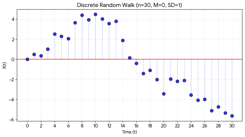
For illustrative purposes, a realization of a discrete random walk based on Gaussian white noise is shown below. The appendix to the article includes an MQL5 script that plots a realization of a random walk based on Gaussian white noise with specified parameters.

Wiener Process

This is a continuous analogue, in both senses, of a discrete random walk. The relationship between them is plain to see: the Wiener process is obtained from its discrete counterpart by taking a limit. Moreover, no matter which discrete noise distribution is used as the basis, the result is always a Gaussian process — this is reminiscent of the Central Limit Theorem (CLT). Properties of the Wiener process under this classification:

• Time and States: A process with continuous time and a continuous state space.
• Increments: It has independent, stationary increments. For any time interval h, the increment has a normal (Gaussian) distribution.
• Stationarity: Like the random walk, the process itself is non-stationary and non-ergodic.
• Characteristics: The expected value is zero (M = 0), and the variance increases linearly with time (D = t). This means that the farther we are from the starting point, the wider the range of possible prices. The autocorrelation function of a Wiener process is given by sqrt(min(t₁, t₂) / max(t₁, t₂)). It also depends on absolute points in time rather than on the difference between them, which once again confirms its non-stationarity.
• Trajectories: this is the “most jagged” of the continuous processes. Its trajectories / sample paths are continuous (there are no discontinuities), but they have no derivative at any point. For a trader, this is mathematical confirmation that a truly random chart has no “instantaneous trend” or velocity vector — the direction changes infinitely often.
• Dependence: it is a Markov process and a classical martingale.

The Wiener process serves as the foundation for all of stochastic financial mathematics, including the Black–Scholes model. The Wiener process is often referred to as Brownian motion or a Brownian process. The reason is that this mathematical model is ideally suited for describing the physical process of the chaotic motion of suspended particles. In the context of financial market analysis, these terms are generally used as complete synonyms.

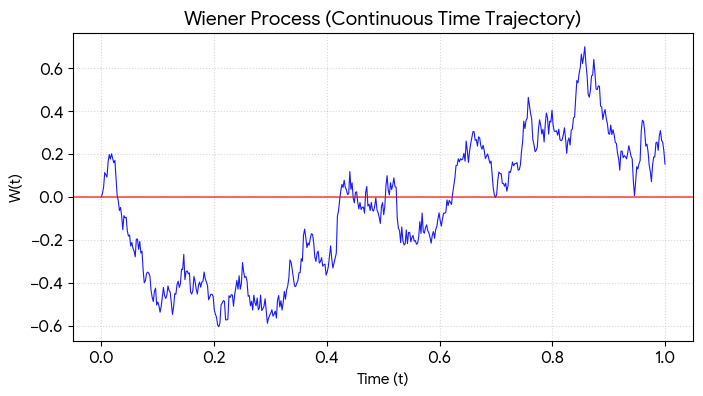
For clarity, a sample path of the Wiener process is shown below. Of course, it would be more accurate to speak of its discretization rather than the sample path itself. The appendix to this article includes an MQL5 script that plots a realization of the Wiener process with a specified variance and sampling frequency.

Like a discrete random walk, the Wiener process is a benchmark model of a market in which it is fundamentally impossible to make money. Mathematically, this means that the equity of any trading system on such a process is inevitably a martingale in continuous time. This means that our expected final account balance will always be equal to the initial capital, no matter how complex the entry and exit algorithms we use may be.

To illustrate this effect, the appendix to the article includes the following:

• a script that simulates the account balance when trading with zero mean using the classic Martingale betting system — doubling the position size after each loss;
• A script that simulates the equity of a trading system based on the “sitting out losses” principle: a fixed take-profit with no stop-loss at all.

Poisson Process

Describes the total number of random events occurring at a certain constant rate. Properties of the Poisson process in this classification:

• Time and states: This is a process with continuous time (an event can occur at any moment) but with a discrete state space (we count the number of events as integers: 1, 2, 3...).
• Increments: It has independent, stationary increments that are distributed according to a Poisson distribution.
• Stationarity: The process is nonstationary (the number of events only increases) and is not ergodic.
• Characteristics: The expected value and variance are equal and grow linearly with time: λ * t (where λ is the rate). The autocorrelation function has the same form as that of a Wiener process: sqrt(min(t₁, t₂) / max(t₁, t₂)).
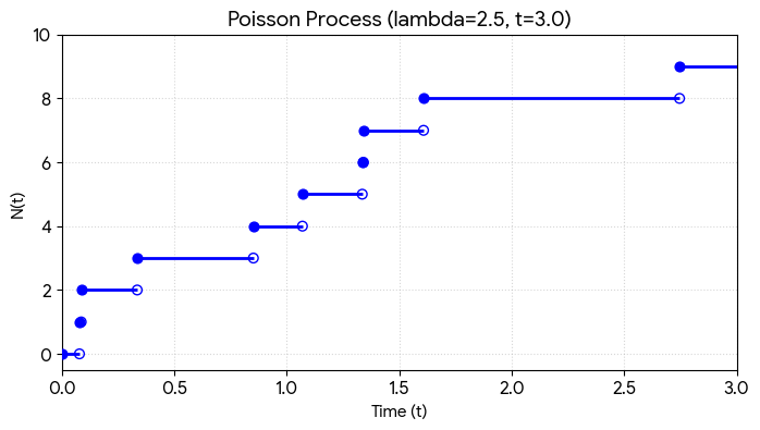
• Trajectories: The sample paths take the form of a staircase with flat steps. The price (or count) remains flat at one level and then jumps sharply upward when an event occurs.
• Dependence: It is a Markov process. If you subtract its mean (trend) from it, the resulting process becomes a martingale.
• Significance for trading: The Poisson process serves as the foundation for market microstructure theory. It is used to model market order flow.

For illustration, a realization of the Poisson process is shown below. The appendix to this article includes an MQL5 script that plots a realization of a Poisson process with a specified intensity.

Markov Chain

In its simplest form, it is a Markov process with discrete time and a discrete state space. Key feature: the transition to the next state depends solely on the system's current state. These transition probabilities are usually represented as a transition probability matrix. In the simplest case (a homogeneous chain), these probabilities do not change over time. In addition to the transition matrix, the probabilities of the initial distribution must be specified to fully describe the chain.

Classification nuances. Many familiar properties no longer apply here, since the states in chains are often not numerical in nature (for example, the states “trend,” “flat,” and “breakout”). In that case, there is no point in calculating the expected value or increments for the state numbers. Other properties, such as ergodicity, depend entirely on the structure of the transition matrix (whether it is possible to eventually reach any other state from any given state).

Applications in trading. Markov chains serve as a basis for predicting candlestick types (for example, the probability of a “bullish” bar after two “bearish” ones). They also form the basis of hidden Markov models (HMMs), which attempt to infer the hidden state of the market (such as high or low volatility) from indirect indicators of price behavior. The appendix to the article contains an MQL5 script that generates a realization of a Markov chain as a sequence of states based on a given transition probability matrix.

Conclusion

We have moved from formalizing the object itself (a process — cross-sections and trajectories), through the concepts of finite-dimensional distributions, moments, and autocovariances, to practical classification (stationarity, increments, independence/uncorrelatedness, the Markov property, martingales, ergodicity) and canonical models (white noise, random walk, Wiener process, Poisson process, Markov chain). For us, the concrete result is not an abstract understanding, but a set of reproducible actions:

• a checklist for describing a series: what exactly is being modeled (price/returns/equity/order flow), discrete or continuous time, type of state space;
• a set of tests to be run before building the model: stationarity (wide-sense/strict), stationarity of increments, autocorrelation, independence of increments, signs of ergodicity;
• benchmark contrasts: comparison of a series with white noise, a random walk, a Wiener process, a Poisson process, or a Markov chain — for intuitive and statistical verification of hypotheses;
• practical tools: ready-made MQL5 scripts in the appendix for generating and visually checking model behavior and typical pitfalls (Martingale strategy, holding through drawdown).

How to apply the results: if the time series is close to stationary and linear, start with econometrics (ARIMA, ACF/PACF, GARCH if necessary); if you need a continuous-time approach or risk management in stochastic differential equations, move on to Itô calculus; when there are clear nonlinearities and regime shifts, consider nonlinear models and regime-switching methods. The next post will move from this map to engineering: econometrics as a practical tool for measuring, filtering, and exploiting the relationships that have been identified.

Appendix: Practical Implementation in Code

It is practically impossible to represent a random process as a single graphical image. The only way to clearly “see” its nature is to generate its sample paths. These trajectories provide a general understanding of the nature of the process, its variability, and its underlying logic. Below are MQL5 scripts that plot realizations of the processes we discussed in the theoretical section. It is helpful to run them in the MetaTrader 5 terminal to see firsthand the difference between the chaos of white noise, the drift of a random walk, and the jumps of a Poisson “staircase.”

Appendix 1

The white_gauss_noise.mq5 script generates a realization of discrete Gaussian white noise with a mean of zero and a specified standard deviation. The main feature of this visualization is the complete absence of lines connecting adjacent points. This is done intentionally: in a discrete-time process, values exist only at fixed points in time, and the lines connecting them would create a false sense of continuity.

Plot of one of the realizations:

Realization of discrete white Gaussian noise with a mean of zero
Specified standard deviation: 1.0
Specified realization length: 30

Appendix 2

The random_walk.mq5 script generates a realization of a discrete random walk based on Gaussian white noise with a mean of zero and a specified standard deviation. It is based on the property of stationary increments: each step of the process is an independent random variable with constant variance. That is precisely why the points on the graph visually form a “line”: the process cannot make a jump greater than the specified standard deviation of a single step allows. However, despite the local proximity of the points, the process remains nonstationary. Due to the accumulation of random deviations, the variance increases linearly over time, and the trajectory can drift very far from its initial level, forming the very “trends” that can mislead us.

Plot of one of the realizations:

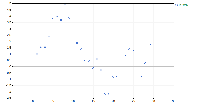
Realization of a discrete random walk based on Gaussian noise with a mean of zero
Specified standard deviation of the noise: 1.0
Specified realization length: 30

Appendix 3

The wiener.mq5 script plots a realization of a Wiener process with the specified variance and sampling rate. The continuity and "jaggedness" of the graph are clearly visible. If you reduce the time interval while keeping the sampling rate the same, the graph will look similar. This indicates its fractal self-similarity. Plot of one of the realizations:

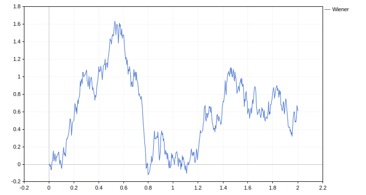
Realization of the Wiener process
Specified standard deviation: 1.0
Specified time interval of the realization: from 0.0 to 2.0
Number of subintervals in the discretization partition: 500

Appendix 4

The martingale.mq5 script plots a realization of a process that models the trading balance with zero mean under the classic Martingale betting system — doubling the position size after each loss (take-profit and stop-loss are equal). The process is discrete in time, since only the moments when trades are closed are considered.

The trajectory of this process consists of long streaks of small gains (slow growth) and sudden deep drawdowns. This script illustrates a paradox: even though the probability of a losing streak is low, its impact on the ending capital is catastrophic. From the perspective of stochastic process theory, the equity of such a system is a martingale with zero expected value. This means that the “beautiful” rising line on the chart is merely temporary behavior of a trajectory that can drop to zero at any moment, confirming the mathematical futility of trying to cheat randomness through simple position sizing. Plot of one of the realizations:

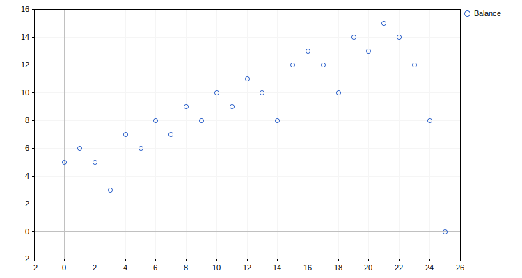
Realization of the trading equity process with doubling after a loss (Martingale betting system)
with equal probabilities of losing and winning
Specified initial capital: 5

Appendix 5

The sitting.mq5 script simulates the equity dynamics of a trading system that operates on a price modeled as a Wiener process, using the “sitting out losses” principle: a fixed take-profit with no stop-loss whatsoever. The process is continuous in time, but for clarity only the points of trade entry, trade exit, and drawdown occurrence are shown.

The process trajectories look surprisingly attractive (up to a certain point): we see an almost perfect rising line made up of small profits. However, this is merely a consequence of the fact that we artificially “select” positive deviations and ignore negative ones until they turn into a catastrophic loss.

Since the underlying process is a martingale, the accumulated equity of such a system also remains a martingale. Mathematically, this means that the total of all realized take-profit gains will sooner or later be wiped out by a single massive drawdown that will reduce the deposit to zero. Plot of one of the realizations:

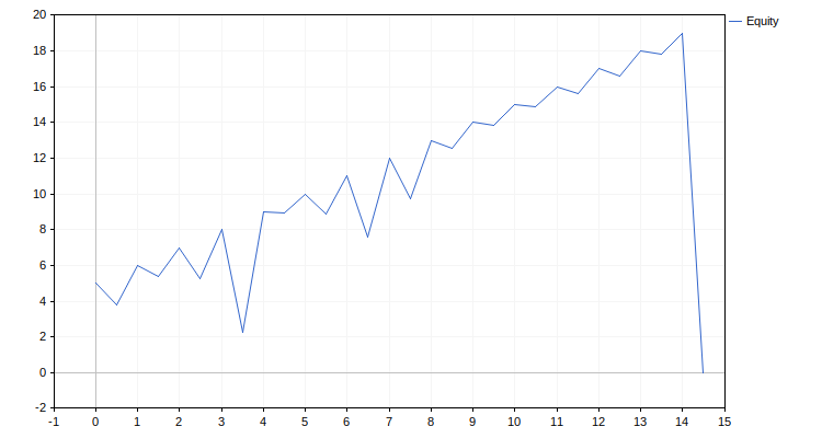
Sample path of the equity process for trading without a stop-loss and with a fixed take-profit,
with the price behaving like a Wiener process
Specified initial capital: 5.0

Appendix 6

The poisson.mq5 script plots a realization of a Poisson process with a specified rate over a specified time interval. Generation is based on a well-known property of the process: the time intervals between events are independent of one another and follow an exponential distribution with a mean equal to the reciprocal of the process rate. Plot of one of the realizations:

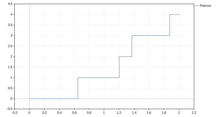
Realization of a Poisson process
Specified intensity: 4.0
Specified time interval for the realization: from 0.0 to 2.0

Appendix 7
The markov_chain.mq5 script generates a realization of a Markov chain as a sequence of states using a given transition probability matrix. One of the run results:

Number of states in the Markov chain: 3
Transition probability matrix:
[[0.70, 0.25, 0.05]
[0.25, 0.70, 0.05]
[0.05, 0.05, 0.90]]
Specified number of transitions: 20
Generated trajectory (sequence of states denoted by their numbers):
1 -> 2 -> 3 -> 3 -> 3 -> 3 -> 1 -> 1 -> 1 -> 1 -> 3 -> 3 -> 2 -> 1 -> 1 -> 1 -> 2 -> 2 -> 2 -> 2 -> 2

List of attached files

#	Name	Description
1	white_gauss_noise.mq5	Discrete Gaussian white noise.
2	random_walk.mq5	Discrete random walk based on Gaussian white noise.
3	wiener.mq5	Wiener process with a specified variance and sampling rate.
4	martingale.mq5	Simulating the trading balance (with zero mean) under the classic Martingale betting system.
5	sitting.mq5	Equity dynamics of a trading system that operates on price (a Wiener process) with a fixed take-profit level and no stop-loss.
6	poisson.mq5	Poisson process with a specified rate over a specified time interval.
7	markov_chain.mq5	Markov chain as a sequence of states based on a given transition probability matrix.