Bayesian Online Change-Point Detection (BOCPD) in MQL5: One Regime-Break Signal, Three Ways to Use It

Introduction

Ask most standard change-detection tools when the market "changed", and they answer in the past tense. A Chow test is handed a fixed block of history and told to find the break that already happened inside it. A CUSUM chart accumulates deviations until, some bars after the fact, the running sum crosses a line. Even the regime classifiers built on autocorrelation or volatility describe the state you are already in, not the moment you left the last one. These are all valuable, and the MQL5 community has produced excellent implementations of them, but they share a stance: look back over a window and decide, retrospectively, where the seam was.

Live trading needs the present tense. When a volatility regime flips or a trend quietly dies, the useful question is not "where, in this old window, was the break?" but "given everything up to this bar and nothing after it, what is the probability that the regime just ended?" That is a fundamentally online question, and it wants a fundamentally online answer: causal, updated every bar, and honest about its own uncertainty.

There is a method built precisely for this, and it is conspicuously absent from the MQL5 landscape. Bayesian Online Change-Point Detection (BOCPD), introduced by Adams and MacKay in 2007, maintains a full probability distribution over one hidden quantity: the run length, the number of bars since the last change-point. Every new observation revises that distribution. When the data stop looking like the current regime, the probability mass collapses back toward a run length of zero, and that collapse is the alarm. No future data, no fixed window, no retrospection. Just a per-bar, probabilistic statement about whether the ground has shifted under your feet.

The point of this article is not to add one more regime detector to a crowded shelf. That shelf is already well stocked with strong work, from a custom regime-detection system built on autocorrelation and volatility to Hidden Markov Models for volatility prediction, and BOCPD is not meant to displace any of them. What it offers instead is a different primitive: rather than classifying which state you are in, it produces the probability that the state just broke, and that one primitive drives three different jobs. We build the model once, as a self-contained class with no external dependencies, and then put it to work three ways: as a live regime monitor you read, as a moving average that resets itself so an indicator can react to breaks internally, and as a risk overlay that de-risks a strategy the moment the market turns dangerous. See it, let an indicator use it, let your account use it.

A note on scope. BOCPD is a change-detection tool, not a direction-prediction tool. It tells you that the statistical character of the series has probably shifted; it does not tell you which way to trade. Everything here is framed accordingly: the monitor reports, the adaptive average adapts, and the overlay controls exposure. None of them predicts direction.

We will cover:

1. Why online change-point detection, and why Bayesian
2. The BOCPD recursion
3. Building the model: the CBOCPD class
4. Use 1: the regime monitor
5. Use 2: the self-resetting adaptive average
6. Use 3: the risk meta-layer
7. Limitations and honest verdict
8. Conclusion

Why online change-point detection, and why Bayesian

It helps to be precise about what "online" buys us, because it is the whole reason for choosing this method over the alternatives already available. Change-point detection splits into two camps. Offline (or retrospective) methods take a fixed batch of data and locate the break points within it after all the data is in hand; they are allowed to use points from after a candidate break to judge it. Online methods process the series one point at a time and must decide, at each step, using only the past, whether a change has just occurred. The MQL5 literature already covers the offline camp well and in depth: the Chow test and the CUSUM of squares for detecting breaks in a cointegrated relationship, and a full suite of SADF-style structural-break tests ported to MQL5. These are excellent tools, but they are offline in spirit, answering questions about a fixed window. BOCPD is online by construction, and that is exactly the stance a chart-side indicator or a live EA occupies.

Fig. 1. Offline detection scans a fixed window after the fact and marks the seam; online detection walks left to right and raises a probability at each new bar using only the past.

Why Bayesian, specifically? Because the honest output of an online detector is not a yes/no flag but a degree of belief, and belief is what Bayesian inference manipulates natively. A frequentist online rule fires when a statistic crosses a threshold, giving a binary event with no calibrated sense of "how sure". BOCPD instead carries a full posterior distribution over the run length and updates it with Bayes' rule as each observation arrives. The quantity we act on, the probability that the regime just changed, falls straight out of that posterior. When the market is calm and settled, the belief that "a change just happened" is low; when the incoming data suddenly stops fitting, that belief rises sharply. We get a continuous, probabilistic alarm rather than a tripwire.

There is a second, subtler reason to prefer the Bayesian formulation here. A change-point can happen in the mean of returns (a trend forming or dying) or in the variance (a volatility regime flipping between calm and turbulent), and for a risk-aware trader the volatility break is often the more important of the two. As we will see, the model we build tracks both the mean and the variance of returns simultaneously, so a break in either one collapses the run-length posterior. A method that watches only the mean would be blind to a pure volatility shift, which is precisely the event that most endangers a strategy assuming stable conditions.

The BOCPD recursion

The whole method rests on one hidden variable. At each time step t we define the run length r_t as the number of steps since the most recent change-point. If a change just occurred, r_t = 0; if the current regime has been running for forty bars, r_t = 40. We never observe the run length directly. What BOCPD computes is the posterior distribution over it, P(r_t | x_1..x_t), given every observation so far. That distribution is the object we carry forward, revise, and read.

Two things can happen at each step:

Between one bar and the next, the run length can only do one of two things. Either the current regime continues, in which case the run length grows by one (r becomes r + 1); or a change-point occurs, in which case the run length resets to zero. The prior probability of the reset is governed by the hazard function. We use the simplest and most common choice, a constant hazard:

H = 1 / lambda

Here lambda is the prior mean regime length in bars, so H is the constant per-bar probability that the current regime ends on this bar. Set lambda to 250 and you are telling the model "in the absence of evidence, expect a regime to last about 250 bars". This single number is the sensitivity dial: a smaller lambda makes the model quicker to suspect a change, a larger one makes it more reluctant.

The predictive model per run length

To judge whether the new observation x_t fits the current regime, we need an explicit model of that regime. We assume that within a regime the observations are drawn from a Gaussian whose mean and precision (the precision is one over the variance) are both unknown but constant. The conjugate prior for a Gaussian with unknown mean and precision is the Normal-Gamma distribution, and conjugacy is what makes the whole method fast: the posterior after seeing data stays in the same family, and the posterior-predictive distribution for the next observation has a closed form. That closed form is a Student-t distribution. For a regime described by Normal-Gamma parameters (mu, kappa, alpha, beta), the predictive density of the next value is a Student-t with

nu = 2*alpha, loc = mu, scale^2 = beta*(kappa + 1) / (alpha*kappa)

where nu is the degrees of freedom. The practical consequence is that scoring a new observation against a regime is a single density evaluation, with no sampling and no iteration. This is what lets BOCPD run bar by bar in real time.

The recursion itself

Now we can state the update that takes the run-length posterior from one step to the next. Adams and MacKay showed that the joint distribution of the run length and the data obeys a simple recursive message-passing rule. Writing the unnormalized message as growth and change-point parts, for each current run length r:

growth: P(r_t = r+1) += P(r_(t-1) = r) * pred(x_t | r) * (1 - H)

changepoint: P(r_t = 0) += P(r_(t-1) = r) * pred(x_t | r) * H

In words: the probability mass currently sitting at run length r is weighted by how well the new observation fits regime r, and then split. Most of it, the fraction (1 - H), flows to run length r + 1, the hypothesis that the regime continued. The rest, the fraction H, contributes to a brand-new run length of zero, the hypothesis that a change-point occurred here. Summing the change-point contribution over every r gives the total mass that lands at r_t = 0. We then renormalize so the distribution sums to one, and finally update each run-length hypothesis' Normal-Gamma parameters with the new observation. That is one full step.

Fig. 2. The run-length posterior. While a regime persists, mass rides a diagonal ridge as the run length grows one bar at a time; when the data stop fitting, the change-point term dumps mass onto run length zero and a new ridge begins.

The Normal-Gamma parameters are updated by the standard single-observation conjugate rule. Given a regime with parameters (mu, kappa, alpha, beta) and a new value x, the updated parameters are:

kappa' = kappa + 1

mu' = (kappa*mu + x) / kappa'

alpha' = alpha + 1/2

beta' = beta + kappa*(x - mu)^2 / (2*kappa')

Each run-length hypothesis carries its own running copy of these four numbers, so hypothesis r always reflects exactly the last r observations. The fresh hypothesis born at each step, run length zero, carries the untouched prior because a brand-new regime has seen no data yet.

Two practical matters remain, and the implementation handles both. First, the exact recursion adds one new run-length hypothesis every step, so the number of hypotheses grows without bound. In practice the posterior mass concentrates on small run lengths, so we cap the tracked run length at a maximum and fold the negligible tail back in, keeping the per-bar cost constant rather than growing with time. Second, multiplying many small probabilities together underflows to zero within a few hundred bars. The cure is to carry everything in log-space and normalize at every step, which is numerically exact and cannot underflow. Both of these live in the class we build next.

Building the model: the CBOCPD class

All of the mathematics above lives in a single reusable header, BOCPDModel.mqh, so that the two indicators and the Expert Advisor can share one source of truth. The class has no external dependencies at all, not even the standard math library: the one special function it needs, the log-gamma, is implemented inside the header. Before any of the recursion, the model declares how it reports its own readiness, because a run-length posterior read before it has seen enough data is dominated by the prior and says nothing.

//--- model status / readiness flag (the honesty mechanism).
//--- The recursion always runs, but the run-length posterior is only
//--- worth reading once enough data has been seen to shape it.
enum ENUM_BOCPD_STATUS
  {
   BOCPD_OK,          // running and warmed up: posterior is meaningful
   BOCPD_NOT_STARTED, // Reset() not called yet
   BOCPD_WARMING_UP,  // fewer than the warm-up count of points seen
   BOCPD_DEGENERATE   // numerical collapse (guarded, should not happen)
  };

The status enum is the same honesty mechanism used across these projects: a reading that has not earned BOCPD_OK is flagged rather than presented as trustworthy. Alongside it sit two constants that encode the practical wrinkles from the previous section, the run-length cap and the warm-up count:

//--- default cap on the tracked run length. The exact Adams-MacKay
//--- recursion grows one run-length hypothesis per bar without bound;
//--- in practice the posterior mass concentrates on small run lengths,
//--- so we truncate at RMAX and fold the tail back to keep cost O(RMAX)
//--- per bar rather than O(t).
#define BOCPD_DEFAULT_RMAX   250
//--- points to observe before the posterior is declared trustworthy.
//--- Below this the Normal-Gamma predictive is dominated by the prior.
#define BOCPD_WARMUP         20

The class stores the configuration, the shared Normal-Gamma prior, one running set of Normal-Gamma parameters per run length, and the run-length distribution itself, held in log-space. The public interface separates one-time configuration from the per-bar Update and from the readouts that consume the posterior.

public:
                     CBOCPD(void);
   //--- one-time configuration. Call before Reset(), or accept the
   //--- constructor defaults. hazardLambda is the prior mean regime
   //--- length in bars (H = 1/lambda).
   void              Configure(const double hazardLambda,const int rmax=BOCPD_DEFAULT_RMAX);
   void              SetPrior(const double mu0,const double kappa0,
                              const double alpha0,const double beta0);
   //--- (re)initialize the recursion to "run length 0, prior belief".
   void              Reset(void);
   //--- feed one observation (e.g. one bar's log return) and advance
   //--- the run-length posterior by a single Adams-MacKay step.
   void              Update(const double x);
   //--- readouts on the current posterior -----------------------------
   double            ChangePointProbability(void) const; // P(run length = 0 now)
   double            ShortRunMass(const int k)   const;  // P(run length <= k) - the detector
   int               MAPRunLength(void)          const;  // most-probable run length
   double            ExpectedRunLength(void)     const;  // posterior-mean run length
   double            RunLengthProb(const int r)  const;  // P(run length = r), linear

The observation model is input-agnostic: Update takes a single double. In every consumer below we feed it one bar's log return, which keeps the series roughly stationary and matches the convention used across these risk articles. The prior defaults are chosen for exactly that input, and are set in the constructor.

//+------------------------------------------------------------------+
//| Construct with sensible defaults: a 250-bar mean regime length,  |
//| a vague, self-scaling Normal-Gamma prior, and the standard cap.  |
//+------------------------------------------------------------------+
CBOCPD::CBOCPD(void)
  {
   m_rmax   = BOCPD_DEFAULT_RMAX;
   m_mu0    = 0.0;    // returns centre on zero
   m_kappa0 = 1.0;    // one pseudo-observation of the mean
   m_alpha0 = 1.0;    // vague precision prior...
   m_beta0  = 1.0e-4; // ...scaled for the tiny variance of log returns
   Configure(250.0,m_rmax);
   m_seen   = 0;
   m_len    = 0;
   m_status = BOCPD_NOT_STARTED;
  }

What the prior actually says

The four Normal-Gamma hyperparameters are not arbitrary knobs; each one is a statement about what we believe before seeing any data, and it pays to read them literally, because they are also the belief a brand-new regime is born with after every change-point. The prior is doing double duty: it is both the starting point of the whole recursion and the template for every fresh regime the model ever hypothesizes.

• mu0 = 0 is the prior mean of the series. Log returns are centered on zero, so a fresh regime starts out expecting no drift until the data say otherwise. This is the natural, assumption-light choice for returns; on a series with a known baseline you would move it.
• kappa0 = 1 is the confidence in that mean, expressed as a count of pseudo-observations. Setting it to one says "my belief that the mean is zero is worth about a single data point", which is deliberately weak: after even a handful of real observations, the data dominate the prior mean. A larger kappa0 would make each fresh regime cling to a zero mean for longer before the evidence could move it.
• alpha0 = 1 is the shape parameter of the Gamma prior on the precision. With alpha0 = 1 the predictive Student-t has nu = 2*alpha0 = 2 degrees of freedom at birth, a genuinely heavy-tailed distribution. That heavy tail is a feature: a newborn regime, having seen almost nothing, should be tolerant of a wide spread of next values rather than confidently narrow, so it does not raise a false change-point on the very next observation.
• beta0 = 1e-4 is the rate parameter, and it is the one value that is genuinely scale-dependent. The prior mean variance implied by the Gamma is beta0/alpha0, so beta0 = 1e-4 with alpha0 = 1 encodes a prior variance of 1e-4, a standard deviation of one percent per bar, which is the right order of magnitude for the log returns of a liquid instrument. This is the single number a caller must rethink when feeding the model a differently scaled series; everything else transfers unchanged.

The word "vague" in the constructor comment is precise, not casual: a vague prior is one weak enough that the data quickly overwhelm it, which is exactly what we want here. We are not trying to inject strong beliefs about the market; we are giving each regime a sensible, self-scaling blank slate and letting the observations shape it. A caller who wants a different posture can override all four values through SetPrior, whose guards keep every parameter in its valid range, but the defaults are tuned to need no such intervention on return data.

This is also why Reset seeds the very first run-length slot with exactly these four numbers and a probability of one. Before any data arrives, the model's entire belief is "we are zero bars into a regime that looks like the prior", and every subsequent structure grows out of that single seed through repeated Update calls.

//--- start with one live slot: r = 0, prior belief, probability 1.
   m_mu[0]    = m_mu0;
   m_kappa[0] = m_kappa0;
   m_alpha[0] = m_alpha0;
   m_beta[0]  = m_beta0;
   m_logP[0]  = 0.0;                 // log(1)
   m_len      = 1;

The single most important line is m_logP[0] = 0.0, because zero is the logarithm of one. The whole recursion lives in log-space, so a probability of one, complete certainty that we are at run length zero, is stored as a log-probability of zero. That convention pervades every readout and every update in the class, and it is the reason the arithmetic never underflows, as we will see next.

The predictive density

Scoring an observation against a regime is the Student-t density derived earlier, evaluated in log-space for stability. The log-gamma terms are what make it numerically well-behaved even for heavy-tailed, low-degree-of-freedom regimes.

//+------------------------------------------------------------------+
//| Log density of the Normal-Gamma posterior-predictive at x. With  |
//| unknown mean and precision, the predictive is a Student-t with   |
//|   nu    = 2*alpha            degrees of freedom,                 |
//|   loc   = mu,                                                    |
//|   scale^2 = beta*(kappa+1) / (alpha*kappa).                      |
//| We evaluate its log density directly; lgamma keeps it stable.    |
//+------------------------------------------------------------------+
double CBOCPD::LogStudentT(const double x,const double mu,
                           const double kappa,const double alpha,
                           const double beta) const
  {
   double nu     = 2.0*alpha;
   double scale2 = beta*(kappa+1.0)/(alpha*kappa);
   if(scale2<=0.0 || nu<=0.0)
      return -1.0e300;                        // degenerate: repel
   double d      = x-mu;
   double arg    = 1.0 + (d*d)/(nu*scale2);   // 1 + t^2/nu
//--- log Student-t:
//---   lgamma((nu+1)/2) - lgamma(nu/2)
//---   - 0.5*log(nu*pi*scale2) - ((nu+1)/2)*log(arg)
   double logc = LogGamma((nu+1.0)*0.5) - LogGamma(nu*0.5)
                 - 0.5*MathLog(nu*M_PI*scale2);
   return logc - 0.5*(nu+1.0)*MathLog(arg);
  }

The guard at the top matters as much as the formula. If a degenerate regime ever produces a non-positive scale or non-positive degrees of freedom, the density is undefined, so the method returns a hugely negative log value rather than a not-a-number. In log-space a return of -1e300 is effectively "this observation is impossible under this regime", which correctly drives that run-length hypothesis's contribution to zero when the messages are combined, instead of letting a NaN poison the entire posterior.

Staying dependency-free: the log-gamma

The Student-t density needs the log of the gamma function, and that is the only non-elementary special function the whole class requires. Rather than pull in a math library for it, we implement it directly in the header with the Lanczos approximation, so BOCPDModel.mqh depends on nothing at all and drops into any project as a single include. This mirrors the self-contained philosophy of the companion EVT engine, which also refused external dependencies.

//+------------------------------------------------------------------+
//| Log of the gamma function via the Lanczos approximation (g=7,    |
//| 9 coefficients). Accurate to ~1e-13 for the positive arguments we|
//| pass here, and self-contained so the header needs no math library|
//+------------------------------------------------------------------+
double CBOCPD::LogGamma(const double z) const
  {
   static const double g=7.0;
   static const double c[9]=
     {
      0.99999999999980993,
      676.5203681218851,
      -1259.1392167224028,
      771.32342877765313,
      -176.61502916214059,
      12.507343278686905,
      -0.13857109526572012,
      9.9843695780195716e-6,
      1.5056327351493116e-7
     };
//--- reflection for z < 0.5 : lgamma(z) = log(pi/sin(pi z)) - lgamma(1-z)
   if(z<0.5)
      return MathLog(M_PI/MathSin(M_PI*z)) - LogGamma(1.0-z);
   double x=z-1.0;
   double a=c[0];
   double t=x+g+0.5;
   for(int i=1;i<9;i++)
      a+=c[i]/(x+i);
   return 0.5*MathLog(2.0*M_PI) + (x+0.5)*MathLog(t) - t + MathLog(a);
  }

The Lanczos approximation is a classic: a short weighted sum of nine fixed coefficients reconstructs the gamma function to roughly thirteen significant digits across the whole positive range we ever evaluate. The reflection formula in the first branch extends it below one-half, which we never actually hit with our arguments but include for correctness and completeness. The practical payoff is that a reader can take this one header, include it, and run BOCPD with no other files, which is exactly the bar a reusable component should clear.

Why log-space, and the log-sum-exp that makes it work

The recursion multiplies a chain of probabilities together, each a small number well below one. Do that in ordinary floating point and within a few hundred bars the product underflows to zero, at which point the posterior is a vector of zeros and the model is dead. The standard cure is to carry everything as logarithms, turning the runaway products into harmless sums. But logarithms create a new problem the moment you need to add two probabilities rather than multiply them. This happens at every step, when the change-point contributions from every run length must be summed into the single r = 0 slot. Adding in log-space means computing the log of a sum of exponentials, and exponentiating a large-magnitude log naively overflows or underflows all over again. The log-sum-exp trick solves this by factoring out the maximum first.

//+------------------------------------------------------------------+
//| Numerically stable log(sum(exp(v[i]))) over the first n entries. |
//| Subtracting the max before exponentiating prevents overflow and  |
//| keeps the normalization exact even when the logs are very small. |
//+------------------------------------------------------------------+
double CBOCPD::LogSumExp(const double &v[],const int n) const
  {
   if(n<=0)
      return -1.0e300;
   double m=v[0];
   for(int i=1;i<n;i++)
      if(v[i]>m)
         m=v[i];
   if(!MathIsValidNumber(m) || m<=-1.0e300)
      return -1.0e300;
   double s=0.0;
   for(int i=0;i<n;i++)
      s+=MathExp(v[i]-m);
   return m+MathLog(s);
  }

The identity being used is that the log of a sum of exponentials equals the maximum log value plus the log of the sum of exponentials of the differences from that maximum. Because every difference v[i] - m is at most zero, every exponential in the loop is at most one, so nothing overflows; and because the largest term contributes exactly one, nothing underflows to a meaningless zero either. This one helper is called at every step, both to fold the change-point contributions into the r = 0 slot and to renormalize the whole posterior, and it is what makes the log-space recursion exact rather than merely approximate. With the predictive density and these two numerical foundations in place, the actual recursion is short.

One step of the recursion

The heart of the class is Update, which performs exactly the growth-and-changepoint split described in the previous section, then advances the sufficient statistics and renormalizes. The first block scores the new value under every live run length and builds the two parts of the message.

//--- 1. predictive log-likelihood of x under each current run length.
   double logPred[];
   ArrayResize(logPred,n);
   for(int r=0;r<n;r++)
      logPred[r]=LogStudentT(x,m_mu[r],m_kappa[r],m_alpha[r],m_beta[r]);
//--- 2. growth: run length r (mass m_logP[r]) continues to r+1.
//---    new index (r+1) inherits the message log P(r) + logPred[r]
//---    + log(1-H). We build the next log-posterior in newLogP.
   int newLen = n+1;
   double newLogP[];
   ArrayResize(newLogP,newLen);
   for(int r=0;r<newLen;r++)
      newLogP[r]=-1.0e300;
   for(int r=0;r<n;r++)
      newLogP[r+1]=m_logP[r]+logPred[r]+m_log_1mh;
//--- 3. changepoint: all live run lengths collapse into the new r=0,
//---    each contributing log P(r) + logPred[r] + log(H). Sum in
//---    log-space via LogSumExp.
   double cpTerms[];
   ArrayResize(cpTerms,n);
   for(int r=0;r<n;r++)
      cpTerms[r]=m_logP[r]+logPred[r]+m_log_h;
   newLogP[0]=LogSumExp(cpTerms,n);

This is where the two abstract equations from the recursion section become concrete lines, and it is worth mapping them one to one, because the correspondence is exact. Recall the growth and change-point messages:

growth: P(r_t = r+1) += P(r_(t-1) = r) * pred(x_t | r) * (1 - H)

changepoint: P(r_t = 0) += P(r_(t-1) = r) * pred(x_t | r) * H

Every multiplication in those formulas is an addition in the code, because we work in logarithms. The growth line, newLogP[r+1] = m_logP[r] + logPred[r] + m_log_1mh, is the growth equation term for term: m_logP[r] is the log of the old mass P(r_(t-1) = r); logPred[r] is the log predictive pred(x_t | r) computed in the first block; and m_log_1mh is the cached log(1 - H). Writing the result into index r+1 is precisely the "the regime continued, so the run length grew by one" statement. The change-point line differs by exactly one symbol, m_log_h in place of m_log_1mh, which is log(H) instead of log(1 - H), and by the fact that every run length feeds the same destination, run length zero. That "every source into one destination" is a summation, and a summation of probabilities held as logs is exactly what LogSumExp is for, which is why the change-point terms are gathered into cpTerms and folded into newLogP[0] with a single stable call. Both hazard logs are precomputed once in Configure rather than recomputed every bar, since the hazard is constant.

The growth term shifts each hypothesis one slot to the right with the (1 - H) weight applied in log-space as an addition of log(1 - H). The change-point term collects every hypothesis, weights it by H, and sums the contributions with a numerically stable log-sum-exp into the new run-length-zero slot. The sufficient-statistics update follows immediately, applying the conjugate rule from the previous section to every carried-forward hypothesis while seeding the new zero slot with the untouched prior.

   for(int r=0;r<n;r++)
     {
      double kappa = m_kappa[r];
      double mu    = m_mu[r];
      double alpha = m_alpha[r];
      double beta  = m_beta[r];
      double kappaP = kappa+1.0;
      double muP    = (kappa*mu + x)/kappaP;
      double alphaP = alpha+0.5;
      double betaP  = beta + (kappa*(x-mu)*(x-mu))/(2.0*kappaP);
      newMu[r+1]    = muP;
      newKappa[r+1] = kappaP;
      newAlpha[r+1] = alphaP;
      newBeta[r+1]  = betaP;
     }

After the split and the statistics update, the method renormalizes the log-posterior and truncates it at the run-length cap. Both operations are visible in the final block.

//--- 5. normalize the new log-posterior so it sums to 1.
   double logNorm = LogSumExp(newLogP,newLen);
   if(!MathIsValidNumber(logNorm) || logNorm<=-1.0e300)
     {
      m_status=BOCPD_DEGENERATE;              // guarded; should not occur
      return;
     }
   for(int r=0;r<newLen;r++)
      newLogP[r]-=logNorm;
//--- 6. truncate at RMAX. Beyond the cap the posterior mass is
//---    negligible; we simply drop the overflow slot and renormalize,
//---    which keeps the per-bar cost bounded.
   int keep = (newLen<=m_rmax+1) ? newLen : m_rmax+1;
   if(keep<newLen)
     {
      double logRenorm = LogSumExp(newLogP,keep);
      for(int r=0;r<keep;r++)
         newLogP[r]-=logRenorm;
     }

Normalization in log-space is a subtraction, not a division: computing the total log-mass with LogSumExp and subtracting it from every entry rescales the distribution to sum to one, exactly and cheaply. The guard around it is the last line of defense; if the total mass ever came back as an invalid number, the model flags itself BOCPD_DEGENERATE and stops rather than propagating garbage, though with the per-regime density guards already in place this branch should never fire.

The truncation is what makes the whole thing real-time. The exact Adams-MacKay recursion adds one run-length hypothesis every bar, so after t bars there are t hypotheses and the cost of each step grows without bound. In practice the posterior mass concentrates on small run lengths, the ones consistent with recent data, and the long tail carries negligible probability. So once the number of live slots exceeds the cap, we simply keep the first RMAX+1 and renormalize what remains. This bounds the work per bar to a constant regardless of how long the chart is, which is precisely what lets the indicators run smoothly over years of history. The committed state, the trimmed log-posterior and its matching per-regime statistics, then becomes the input to the next bar's step.

Reading the posterior: why the obvious readout is the wrong one

With the recursion in place, the question is what to actually read off it as "a change just happened". The tempting answer is the probability mass sitting exactly at run length zero, and the class exposes it as ChangePointProbability. But that reading is misleading, and the reason is worth understanding. At every single step, the change-point term injects a fixed fraction H of the mass into run length zero, and on the very next step almost all of it flows on to run length one. So the raw run-length-zero mass barely moves; it mostly reflects the constant hazard, not the evidence. The real signal that a regime just broke is mass piling up on the smallest run lengths, because a genuine change-point makes short runs suddenly far more plausible than the long run the model had been riding. The correct detector is therefore the cumulative mass on run lengths up to a small horizon k, exposed as ShortRunMass.

//+------------------------------------------------------------------+
//| Posterior mass on short run lengths: P(run length <= k). This is |
//| the practical change-point detector. The instantaneous r=0 mass  |
//| only ever holds a single bar's hazard inflow before it grows to  |
//| r=1, so on its own it barely moves; the real evidence that a     |
//| regime just broke is mass PILING UP on the smallest run lengths. |
//| A spike in ShortRunMass(k) is what "a change just happened" looks|
//| like, with k trading detection lag against false alarms.         |
//+------------------------------------------------------------------+
double CBOCPD::ShortRunMass(const int k) const
  {
   if(m_len<=0)
      return 0.0;
   int top=(k<m_len-1)?k:m_len-1;
   double s=0.0;
   for(int r=0;r<=top;r++)
      s+=MathExp(m_logP[r]);
   return s;
  }

The horizon k is a small tunable trade-off: a smaller k reacts faster but only to sharp breaks, a larger k catches subtler shifts at the cost of a little more lag. Across all three consumers below we use k = 5 with an alert level around 0.35, which fires cleanly on real regime breaks while staying quiet during calm stretches. The companion readout ExpectedRunLength, the posterior-mean run length, is the smooth mirror image: it ramps steadily upward while a regime persists and collapses toward zero the instant the detector fires, which makes it a natural "how settled is the market" line to plot alongside the alarm.

Use 1: the regime monitor

The first and simplest thing to do with the primitive is to look at it. The indicator BOCPDRegime.mq5 runs the model on the log-return stream and, in a sub-window, plots the two readouts that matter: the change-point detector ShortRunMass, which spikes when the regime breaks, and the normalized expected run length, which ramps while a regime holds and collapses at a break. It also drops a marker where the detector crosses the alert level, and reports the live reading in a small panel.

The engine is advanced incrementally. BOCPD is a causal forward recursion, so its state carries forward naturally from bar to bar; there is no need to recompute history on every tick. The indicator feeds the model only the closed-bar returns it has not yet seen, which keeps the per-tick cost at one recursion step rather than one per bar of the whole chart. This matters: an early version that replayed the entire history on each call was unusably slow, and the fix is exactly this incremental discipline.

//--- Only CLOSED bars feed the recursion: BOCPD's Update is irreversible
//--- (it advances the posterior), so the still-forming last bar must not
//--- be consumed until it closes. logret[0..nret-2] are closed-bar
//--- returns; logret[nret-1] belongs to the forming bar.
   int lastClosedRet = nret-1;              // count of closed-bar returns
//--- on a fresh load restart the recursion.
   if(prev_calculated==0)
     {
      g_bocpd.Reset();
      g_done=0;
      PcpBuffer[0]=EMPTY_VALUE;
      RunLenBuffer[0]=EMPTY_VALUE;
      MarkBuffer[0]=EMPTY_VALUE;
     }

One subtlety drives the "closed bars only" rule: unlike an ordinary indicator calculation, a BOCPD Update is irreversible. Feeding a value advances the posterior permanently, so we cannot feed the still-forming bar and then "take it back" when its price changes on the next tick. The model therefore consumes a bar only once it has closed; the forming bar simply carries the last closed reading forward so the plotted line does not blank at the right edge. Each closed bar that arrives is scored, and the two buffers plus the marker are filled from the model's readouts.

//--- append only the closed-bar returns the model has not yet seen.
   for(int i=g_done;i<lastClosedRet;i++)
     {
      g_bocpd.Update(logret[i]);
      int bar=i+1;                                               // return i lands on bar i+1
      if(g_bocpd.IsReady())
        {
         double pcp   = g_bocpd.ShortRunMass(DetectK);
         double eRunB = g_bocpd.ExpectedRunLength();
         double eRunN = eRunB*g_invCap;
         if(eRunN>1.0)
            eRunN=1.0;
         PcpBuffer[bar]   = pcp;
         RunLenBuffer[bar]= eRunN;
         MarkBuffer[bar]  = (pcp>=AlertLevel)?pcp:EMPTY_VALUE;   // dot on alerts
         lastPcp=pcp;
         lastRunBars=eRunB;
        }
      else
        {
         PcpBuffer[bar]   = EMPTY_VALUE;
         RunLenBuffer[bar]= EMPTY_VALUE;
         MarkBuffer[bar]  = EMPTY_VALUE;
        }
     }

Two bookkeeping details in that loop are what make the incremental scheme correct. The counter g_done records how many closed-bar returns the model has already consumed, so on each call the loop starts at g_done and processes only genuinely new bars; after the loop it is advanced to lastClosedRet. And while the model is still in its warm-up window, the IsReady check keeps the buffers empty rather than plotting a posterior dominated by the prior, so the lines simply do not begin until the reading is trustworthy, in the same spirit as the EVT gauge refusing to print a number it cannot stand behind. The forming bar is handled just after the loop: it is not fed to the model, but its buffer slots copy the last closed reading forward so the plotted lines reach the right edge of the chart instead of stopping one bar short.

The panel is a small on-chart readout built from ordinary label objects, refreshed each calculation by a helper, UpdatePanel, which receives the latest change-point probability and expected run length from the loop above. It reports that probability, the expected run length in bars, and a state line, and it color-codes the state so the transition is impossible to miss.

   ObjectSetString(0,g_prefix+"state",OBJPROP_TEXT,
                   g_bocpd.IsReady()
                   ? ((pcp>=AlertLevel)?"state: CHANGE-POINT":"state: stable")
                   : ("state: "+g_bocpd.StatusText()));
   ObjectSetInteger(0,g_prefix+"state",OBJPROP_COLOR,
                    (!g_bocpd.IsReady())?clrSilver:
                    ((pcp>=AlertLevel)?clrOrangeRed:clrLimeGreen));

The three-way conditional is the honesty mechanism surfacing at the display layer. Until the model is ready it shows the warm-up status in grey, taken straight from StatusText; once ready, it reads green "stable" while the change-point probability is below the alert level and red "CHANGE-POINT" the instant it crosses. The same value that drives the plotted line and every downstream decision drives the color, so the panel can never show a calm green while the detector is actually firing.

On a chart, the behavior is exactly what the theory promises. Through calm, settled stretches the change-point line hugs the floor and the run-length line climbs steadily. When a genuine break arrives, a sharp adverse move that no longer fits the prevailing regime, the change-point line spikes hard toward one, the run-length line collapses, and a marker is dropped. The panel flips from a green "stable" to a red "change-point" reading at the same instant.

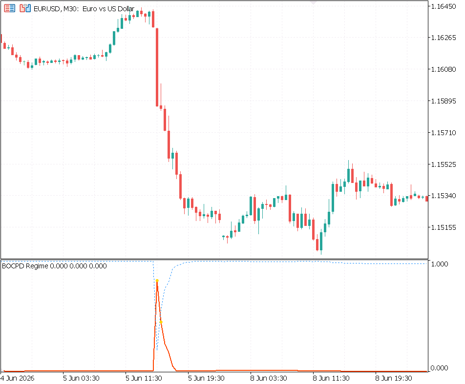
Fig. 3. The regime monitor on EURUSD M30. At the sharp drop, the change-point detector (orange) spikes and the expected run length (blue, dotted) collapses; through the calm stretches both lines rest, correctly signalling no break.

Read as a monitor rather than a signal, the value is that you can watch the market's structural stability directly. A rising change-point line is not a reason to trade in any direction; it is a statement that the assumptions your other tools rest on may have just expired. That statement is useful on its own, but it becomes far more useful when another piece of code consumes it automatically, which is the next two sections.

Use 2: the self-resetting adaptive average

Every trader who has watched a moving average through a sharp move knows its central flaw. A fixed-window average is, by definition, a blend of the last N bars, so immediately after a regime break it is still mostly composed of pre-break prices. It drifts slowly toward the new level, lagging worst at exactly the moment you most need it to be current. The lag is not a tuning problem; it is structural, because the window straddles the boundary between two regimes and averages across it.

BOCPD offers a clean fix. If we know, per bar, when the regime broke, we can make the average forget everything before the break. The indicator BOCPDAdaptiveMA.mq5 does exactly this. It plots two curves on the price chart: an ordinary fixed-window mean, and an adaptive mean whose window is clamped to start at the most recent detected change-point. When the detector fires, the regime start jumps to the current bar, and the adaptive mean is re-seeded from post-break prices only. The consumer of the change-point primitive here is not your eyes but another indicator's internal state.

   for(int i=g_done;i<lastClosedRet;i++)
     {
      g_bocpd.Update(logret[i]);
      int bar=i+1;                                 // return i lands on bar i+1
      //--- a change-point flushes the adaptive window: the new regime
      //--- starts here, so the adaptive mean forgets everything before.
      bool fired=false;
      if(g_bocpd.IsReady() && g_bocpd.ShortRunMass(DetectK)>=AlertLevel)
        {
         g_regimeStart=bar;
         fired=true;
        }
      //--- fixed SMA: always the last MaxWindow bars, regardless of regime
      int fFrom=bar-MaxWindow+1;
      if(fFrom<0) fFrom=0;
      FixedBuffer[bar]=MeanOf(price,fFrom,bar);
      //--- adaptive mean: window starts at the regime start, but never
      //--- reaches back further than MaxWindow bars (so a very old regime
      //--- still behaves like a bounded moving average, not a cumulative one).
      int aFrom=g_regimeStart;
      if(bar-aFrom+1>MaxWindow)
         aFrom=bar-MaxWindow+1;
      if(aFrom<0) aFrom=0;
      AdaptBuffer[bar]=MeanOf(price,aFrom,bar);
      MarkBuffer[bar]=fired?price[bar]:EMPTY_VALUE;
     }

The logic is deliberately transparent, and the two window calculations sit side by side so the contrast is legible. Both means are computed by the same trivial helper, MeanOf, which averages the prices between two bar indices inclusive; the only thing that differs between the fixed and adaptive curves is where each window starts.

The fixed mean always starts its window MaxWindow-1 bars back from the current bar, ignoring regime structure entirely; it is an ordinary simple moving average. The adaptive mean starts its window at g_regimeStart, the bar of the most recent detected change-point. Right after a break, that window is short and composed entirely of new-regime prices, so the adaptive mean sits squarely on the new level while the fixed mean is still half-full of stale ones. As the new regime ages, g_regimeStart stays put and the adaptive window grows bar by bar, until it hits the same MaxWindow length, after which the two curves are identical again.

That cap is the subtle part, and it is exactly the clamp in the code, if(bar - aFrom + 1 > MaxWindow) aFrom = bar - MaxWindow + 1. Without it, a regime that lasts a thousand bars would give the adaptive mean a thousand-bar window, turning it into an ever-lengthening cumulative average that becomes more sluggish the longer the regime runs, the opposite of what a moving average should do. With the clamp, the adaptive mean is guaranteed to be a normal bounded moving average of at most MaxWindow bars; its only departure from the fixed version is that it refuses to let its window straddle a regime boundary. So the two curves are the same object with a single difference, and any gap between them on the chart is attributable entirely to that one design choice, which makes the comparison clean rather than confounded.

The payoff is entirely visual, and it is striking. On a chart with a clear regime break, the two curves tell the whole story on their own.

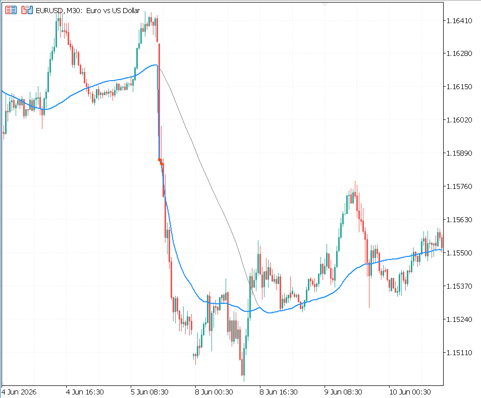
Fig. 4. Fixed mean (grey) versus BOCPD-adaptive mean (blue) through a sharp drop. The change-point marker fires at the top of the move; the adaptive mean re-seeds and reaches the new level within a handful of bars, while the fixed mean glides down slowly, only catching up days later.

At the break, the fixed mean peels away on a long, slow diagonal, taking many bars to arrive at the new price level because it is still dragging the old regime's prices through its window. The adaptive mean flushes at the change-point and reaches the new level almost immediately. Through the calm stretches on either side, where the detector stays quiet, the two curves sit on top of each other, which is exactly correct: with no regime break, there is nothing to adapt to. No backtest is needed to make the point; the gap between the two lines through the transition is the argument.

Use 3: the risk meta-layer

The third use puts the primitive to work on real money. The Expert Advisor BOCPDRiskOverlay.mq5 wraps BOCPD around a deliberately trivial strategy, a moving-average cross, and uses the change-point signal as a risk meta-layer: for a short cooldown after each detected break, it de-risks. The entry logic is not the point and is not meant to be good; the point is the overlay sitting on top of it. This mirrors the structure of the EVT risk overlay from the companion article, where a trivial entry is held constant so that the overlay is the only thing under study.

The critical design decision is that the EA runs in one of three modes, and the three exist to separate signal from side-effect.

//--- risk-overlay mode
enum ENUM_RISK_MODE
  {
   RISK_NONE,     // baseline: overlay off, always full size
   RISK_BOCPD,    // de-risk during cooldown after a BOCPD change-point
   RISK_RANDOM    // de-risk on random cooldowns of matched frequency (control)
  };

The reason for the third mode deserves emphasis, because it is what makes the result honest. Any rule that de-risks will trade less, and trading less in a losing strategy tends to lose less. So a simple "baseline versus BOCPD" comparison cannot, on its own, prove that the change-point timing carried any information; the improvement could be nothing more than reduced exposure. The RISK_RANDOM mode is the control that closes this gap. It de-risks on randomly timed cooldowns of the same average frequency as the BOCPD alarm, so it does roughly the same amount of de-risking, just at the wrong moments. If BOCPD beats random-timed de-risking of matched frequency, then the timing, not merely the reduced exposure, is what did the work.

The overlay is advanced once per bar, before the entry check. It feeds the just-closed bar's return into the model, counts down any active cooldown, and then, depending on the mode, decides whether to arm a fresh one.

void UpdateOverlay()
  {
//--- log return of the just-closed bar (shift 1 vs shift 2)
   double c[2];
   if(CopyClose(_Symbol,_Period,1,2,c)<2)      // c[0]=older @2, c[1]=newer @1
      return;
   if(c[0]<=0.0 || c[1]<=0.0)
      return;
   double r=MathLog(c[1]/c[0]);
   g_bocpd.Update(r);
//--- count down any active cooldown first
   if(g_cooldown>0)
      g_cooldown--;
   if(RiskMode==RISK_BOCPD)
     {
      if(g_bocpd.IsReady() && g_bocpd.ShortRunMass(DetectK)>=AlertLevel)
         g_cooldown=CooldownBars;              // (re)arm on a detected break
     }
   else
      if(RiskMode==RISK_RANDOM)
        {
         //--- independent coin flip: matched average frequency, random timing
         double u=(MathRand()+0.5)/32768.0;
         if(u<g_randHazard)
            g_cooldown=CooldownBars;
        }
  }

The random control's per-bar trigger probability is set to 1/lambda, the same hazard the BOCPD alarm is expected to fire at, so that over a run the two modes arm a comparable number of cooldown episodes. The de-risk action itself is a size multiplier applied during the cooldown; with the default factor of zero, de-risking means simply skipping new entries while the cooldown is active.

//+------------------------------------------------------------------+
//| Size the position given the overlay state. Full base lot normally|
//| during a de-risk cooldown the lot is scaled by DeriskFactor (0 = |
//| skip the trade entirely). Baseline mode always returns base lot. |
//+------------------------------------------------------------------+
double OverlayLot()
  {
   if(RiskMode==RISK_NONE)
      return BaseLot;
   if(g_cooldown>0)
      return BaseLot*DeriskFactor;             // de-risked (0 => no trade)
   return BaseLot;
  }

The overlay is advanced on every new bar even while a position is open, so the model and the cooldown never go stale, and only then is the entry logic consulted. The full OnTick checks the moving-average cross, lets the overlay size or veto the trade, and opens the position if a non-zero lot survives.

void OnTick()
  {
   if(!NewBar())
      return;
//--- always advance the change-point model / cooldown on the new bar,
//--- even while a position is open, so state never goes stale.
   UpdateOverlay();
   if(PositionSelect(_Symbol))
      return;                                  // one position at a time
//--- read the two MAs on the last closed bars (index 0 = older @2)
   double f[2],s[2];
   if(CopyBuffer(g_hFast,0,1,2,f)<2)
      return;
   if(CopyBuffer(g_hSlow,0,1,2,s)<2)
      return;
   bool crossUp  = (f[0]<=s[0] && f[1]>s[1]);
   bool crossDown= (f[0]>=s[0] && f[1]<s[1]);
   if(!crossUp && !crossDown)
      return;
//--- overlay decides size / veto
   double lot=NormalizeLot(OverlayLot());
   if(lot<=0.0)
      return;

The comparison

We run the EA three times over the same history on EURUSD M30, changing only the mode: baseline, BOCPD overlay, and the random control. Everything else is held fixed. The results are summarized below.

Metric	Baseline (None)	BOCPD overlay	Random control
Total net profit	-283.80	-283.40	-434.20
Profit factor	0.89	0.89	0.83
Expected payoff	-2.93	-3.05	-4.52
Recovery factor	-0.33	-0.38	-0.43
Sharpe ratio	-0.80	-0.84	-1.25
Balance drawdown maximal	817.80 (8.06%)	717.60 (7.07%)	968.20 (9.54%)
Equity drawdown maximal	856.50 (8.42%)	755.60 (7.42%)	1006.90 (9.89%)
Total trades	97	93	96

Three readings come out of this table, and together they are the result.

First, against the baseline, BOCPD cut maximum drawdown by about twelve percent, from 856.50 to 755.60 in equity terms, and it did so by skipping only four trades out of ninety-seven. That is a large reduction in downside for a very small reduction in activity, which is the signature of well-timed de-risking rather than blunt throttling.

Second, and this is the point of the whole three-way design, the random control makes everything worse. De-risking at random times, at the same average frequency as the BOCPD alarm, deepened maximum drawdown to 1006.90, well past even the baseline, and dragged the Sharpe ratio from -0.80 down to -1.25. The random control skipped a comparable number of trades to BOCPD, yet produced the opposite effect. This is the evidence that survives scrutiny: BOCPD did not help merely by trading less, because trading less at the wrong moments actively hurt. The timing of the de-risking is what carried the information.

Third, and stated plainly, all three modes still lose money. The moving-average cross is a placeholder, not an edge, and BOCPD does not turn a losing system into a winning one. The only claim the data supports is the narrow, real one: BOCPD-timed de-risking reduced drawdown relative to both doing nothing and de-risking at random. It controls when to step back from risk; it does not manufacture return.

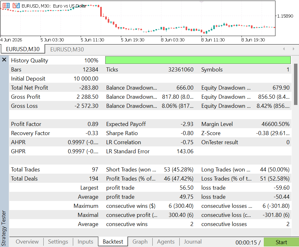
Fig. 5. Baseline equity curve (RiskMode = None): the strategy with no overlay.

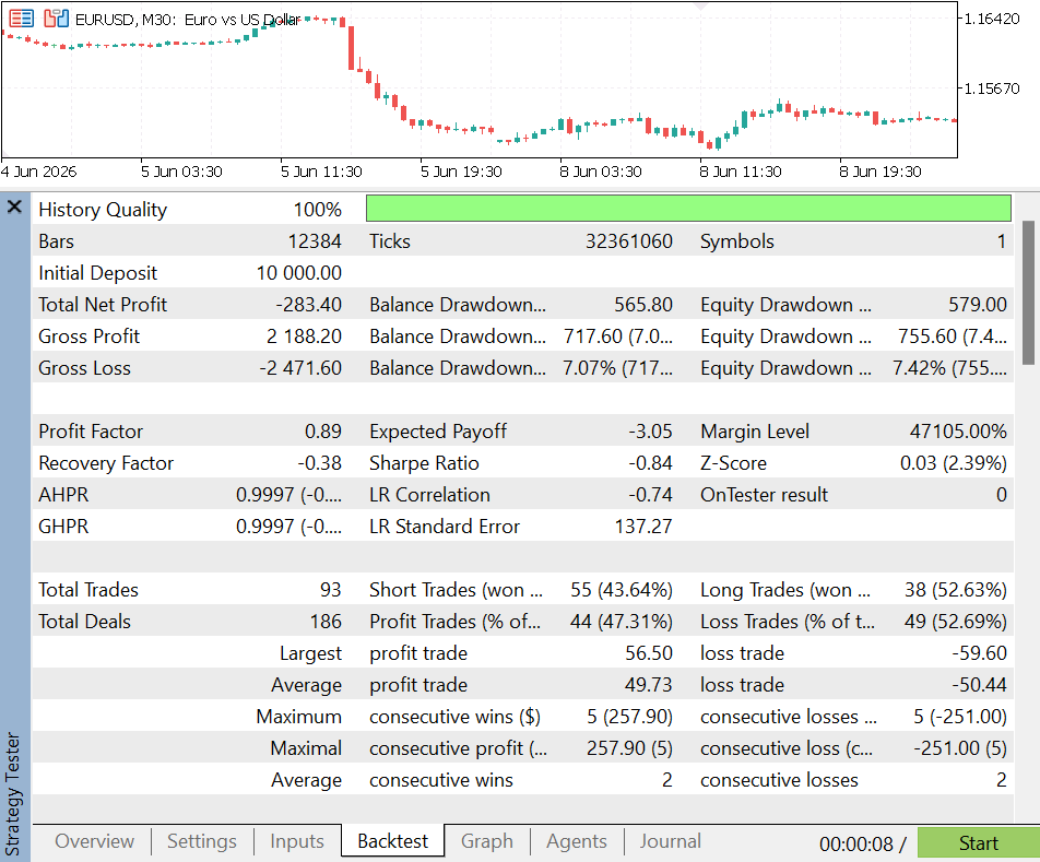
Fig. 6. BOCPD overlay equity curve (RiskMode = BOCPD): the same entries, de-risked for a cooldown after each detected change-point, producing a shallower drawdown.

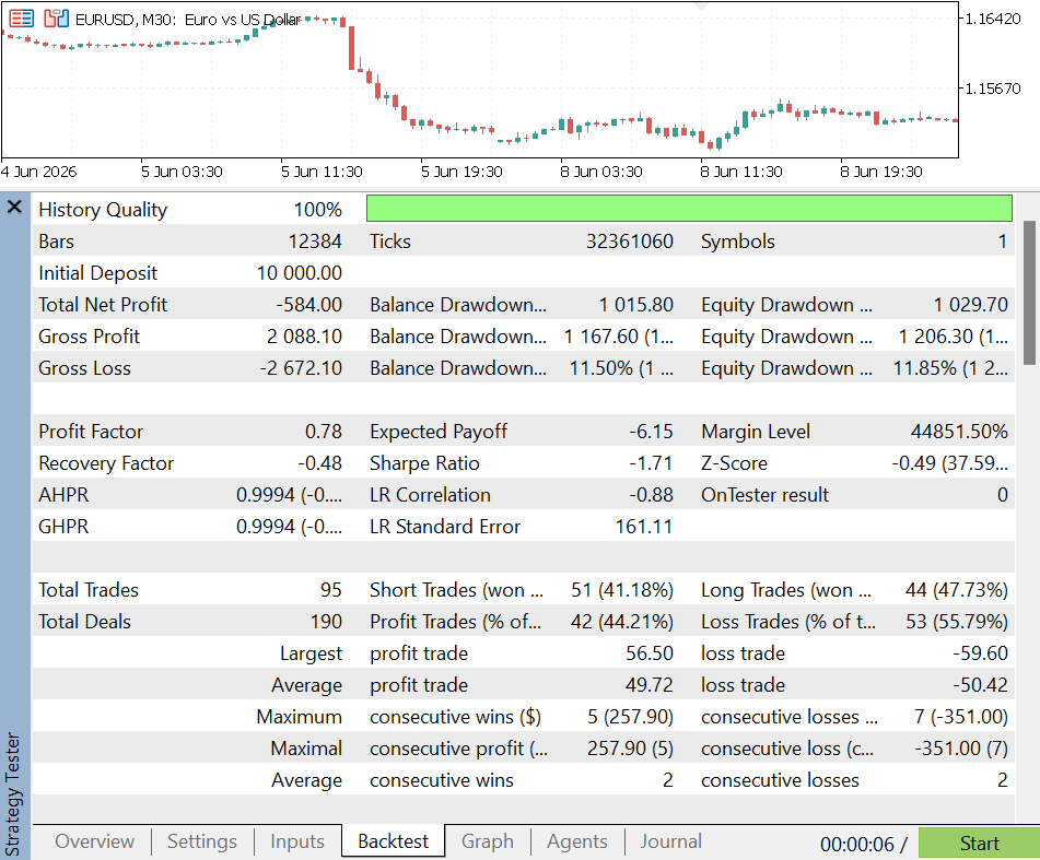
Fig. 7. Random control equity curve (RiskMode = Random): de-risking of matched frequency but random timing, which deepens the drawdown and confirms that BOCPD's timing carried the information.

Note: The random control mode uses a pseudo-random draw, so its exact figures shift slightly from run to run. The direction of the result, random-timed de-risking underperforming both the baseline and the BOCPD overlay, is stable across runs; the specific numbers above are one representative run.

Limitations and honest verdict

BOCPD earns a place in the toolkit, but like any statistical instrument it has a domain where it works and edges where it does not, and using it well means knowing them.

• It detects in proportion to a break's statistical strength. A sharp change, especially a volatility jump, collapses the run-length posterior almost immediately, within a bar or two. A subtle shift, such as a small change in the mean of returns arriving on top of a long, confident regime, is detected slowly or, if it is small enough relative to the noise, not at all. This is not a defect to be tuned away; it is correct Bayesian behavior. A model that fired on every small wobble would be crying wolf, and its alarms would be worthless. The flip side is that BOCPD is inherently better at catching the dramatic, dangerous breaks than the quiet, gradual ones.
• The effect in the overlay rests on relatively few trades. Over the tested window, the difference between the BOCPD overlay and the baseline came down to a handful of well-timed skips. The result is real and the control confirms it, but a handful of trades is a thin base, and the effect would firm up considerably over a longer history containing more regime breaks, or on a more volatile instrument where breaks are frequent and consequential. On a placid series with few genuine regime changes, the overlay has little to do and little to show.
• It measures change, not direction. This bears repeating because it is the most common way such a tool is misread. A spike in the change-point probability says the statistical character of the series has probably shifted; it says nothing about which way price will go next. Treating a change-point as an entry signal is a misuse. The three consumers here are all built to respect this: one reports, one adapts an average, and one controls exposure. None predicts direction.
• It depends on a hazard and a prior. The mean regime length lambda and the Normal-Gamma prior are inputs, and while the defaults suit log returns across liquid instruments, a very different series, or a deliberately faster or slower sensitivity, calls for tuning them. The detector horizon and alert level likewise trade responsiveness against false alarms. These are exposed as inputs precisely so they can be studied rather than trusted blindly.

Within those limits, the verdict is positive. BOCPD fills a real and previously empty slot in the MQL5 landscape: a principled, online, probabilistic statement about when the market's regime has changed, computed causally and cheaply enough to run live. As the three consumers showed, that one primitive is genuinely versatile: you can watch it, you can let an indicator reset itself on it, and you can let it govern when a strategy steps back from risk. It is not a crystal ball, and it is not a source of edge. It is a measurement of structural change, and the right way to act on a measurement is to adapt to it, not to bet direction on it.

Conclusion

We set out to bring Bayesian Online Change-Point Detection to MetaTrader 5, and to show it as a versatile primitive rather than one more regime detector. Along the way we built a complete, self-contained change-detection stack.

• A reusable model. The CBOCPD class implements the Adams-MacKay recursion with a Normal-Gamma conjugate observation model, entirely in log-space and with no external dependencies, so a break in either the mean or the variance of returns collapses the run-length posterior. It exposes the change-point detector and the run-length readouts, and flags its own warm-up rather than reporting a posterior it cannot stand behind.
• A live regime monitor. The first indicator turns the model into an on-chart reading, plotting the change-point detector and the expected run length, marking detected breaks, and updating incrementally so it runs cheaply in real time.
• A self-resetting adaptive average. The second indicator lets another piece of code consume the primitive internally: a moving average that flushes its window on a detected change-point and so snaps to a new regime within a couple of bars, where a fixed-window average lags for many.
• A risk meta-layer. The Expert Advisor uses the change-point signal to de-risk a trivial strategy for a cooldown after each break, and a random-timed control of matched frequency shows that it is the timing, not merely the reduced exposure, that cut drawdown.

The throughline is that BOCPD produces one thing, a per-bar probability that the regime just broke, and that one thing is worth building well because so many different tools can consume it. See it, let an indicator use it, let your account use it. The natural extensions, from richer observation models to multivariate change detection across several instruments, are left as directions for further work.

The programs presented in this article are intended for educational purposes only. Trading carries a high level of risk, and past performance, including backtested results, is not indicative of future results. Always test thoroughly on a demo account before risking real capital.

Getting the Source Code via MQL5 Algo Forge

All source files are attached to this article below, but the full repository is also available on MQL5 Algo Forge, the community's Git-based platform for sharing and collaborating on trading projects.

File name	Description
MQL5\Include\BOCPD\BOCPDModel.mqh	Bayesian Online Change-Point Detection model: the Adams-MacKay recursion with a Normal-Gamma conjugate observation model, log-space and dependency-free
MQL5\Indicators\BOCPD\BOCPDRegime.mq5	The regime monitor: plots the change-point detector and expected run length with break markers and a live reading panel
MQL5\Indicators\BOCPD\BOCPDAdaptiveMA.mq5	The self-resetting adaptive average: a moving average that flushes its window on a detected change-point, drawn against a fixed-window mean
MQL5\Experts\BOCPD\BOCPDRiskOverlay.mq5	The risk meta-layer: an Expert Advisor that de-risks a trivial strategy after each detected change-point, with baseline, BOCPD, and random-control modes