Execution Cost and Slippage Sensitivity Analyzer

Introduction

I once had a strategy that looked ready to trade. Over a two-year backtest, it showed a net profit above two thousand units, a profit factor near 1.6, and a win rate of 61%. The equity curve climbed in a calm, believable line. I funded a small account, switched it on, and watched the live result drift below the backtest week after week. Nothing was broken in the logic. The gap was cost. Each trade paid slightly more spread and slippage, plus a commission the backtest had treated as an afterthought. Those small amounts added up and consumed most of the edge.

This article asks one question: how much execution cost can a strategy absorb before its edge disappears? Net profit and profit factor are measured at the cost the backtest happened to assume. They do not tell you how close that result sits to the cost line or how much the spread would have to widen before a winning system turns into a losing one. A strategy with a wide margin over costs is one you can trade through a noisy broker and a fast market. A strategy that only wins because the test was cheap will not survive contact with a real account.

In this article, we build a script that reads closing deals and measures how robust the results are to execution costs. By the end, you will have a working analyzer that

• Computes the breakeven cost per deal, the cost level at which the net profit reaches zero.
• Reports the cushion, the multiple of an assumed realistic cost that the edge can absorb before it is gone.
• Re-prices the whole record under a rising cost and shows the net profit and profit factor at each level.
• Counts the winning deals that a realistic cost turns into losers and the gross profit that sits close to the cost line.
• Combines these into a single cost-robustness score, graded from A+ to F, with written recommendations.

Everything runs natively inside MetaTrader 5. There are no external libraries, no Python, and no machine learning. The whole tool is a single MQL5 script plus three standalone modules and a small helper that exports the deals from a backtest.

Why a Backtest Understates Costs

A backtest charges the costs you tell it to charge. The spread is often a fixed, optimistic value; commission may be left at zero; and slippage, the difference between the price you wanted and the price you got, is usually absent because the tester fills you at the modeled price. Live trading is not so kind. Spreads widen around news and at the session close. Fast markets fill market orders a few points away from the screen. A broker that looked cheap on a quiet pair can be expensive on the one you actually trade.

The damage is largest where it is hardest to see, on strategies that trade often for small gains. Consider two systems with the same net profit over the same number of deals. One earns its profit from a few large moves; the other scalps many small winners. Add two units of cost to every deal, and the first barely notices, while the second can lose its entire edge. The headline figures are identical, yet one is robust to costs and the other is fragile. Measuring that fragility before you trade is the point of this tool.

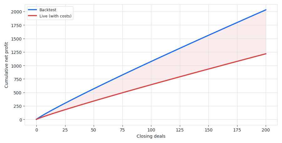
Fig. 1. The same strategy earns less once realistic execution costs are charged on every deal.

What Cost Sensitivity Measures

Before writing code, we need to define the measurements the analyzer reports. The tool models the execution cost of a single closing deal as a fixed part plus a part that scales with the deal volume:

Cost per deal = Fixed + (CostPerLot * Volume)

The fixed part stands for a per-ticket charge such as a minimum commission. The per-lot part stands for the spread, the variable commission, and the slippage, all of which grow with position size. This is a deliberately linear approximation. In reality, spread and slippage also depend on the instrument and on volatility, not on volume alone, but a linear model keeps the estimate transparent and configurable. With the default of 12 units per lot and no fixed part, a 0.50-lot deal pays 6 units, and a 0.10-lot deal pays 1.2 units.

Edge per deal and the breakeven cost. The net profit spread across the deals gives the average edge each deal carries:

Edge per deal = (Net profit) / (Number of deals)

Because every deal pays the same modeled cost on top of its result, the net profit after a cost c is simply the net before cost minus c for every deal. The net reaches zero when c equals the average edge. That value is the breakeven cost per deal: the most each deal can pay, on average, before the edge is gone.

The cushion. A breakeven figure on its own does not say whether it is comfortable or tight. The cushion compares the breakeven cost to the cost you actually expect to pay. It is the multiple of the assumed cost at which the net profit hits zero:

Cushion = (Net profit) / (Total assumed cost)

A cushion of 3.0 means the edge survives costs up to three times what you assumed. A cushion near 1.0 means your assumed cost already eats the whole edge. The retention, the share of the net profit that survives at the assumed cost, follows directly from the cushion:

Retention = 1 - (1 / Cushion)

Because retention is fixed once the cushion is known, the score grades the cushion directly and reports retention only as an intuitive companion.

The profit factor at the assumed cost. The cushion is an aggregate. Two records with the same cushion can degrade differently depending on how their winners and losers sit relative to the cost. So the analyzer also re-prices every deal at the assumed cost and recomputes the profit factor. A deal that was a small winner can become a loser, which both lowers gross profit and raises gross loss. The drop from the profit factor before cost to the profit factor at cost measures how the whole distribution holds up, not just the sum.

Win erosion and thin winners. The most fragile profit is the profit that sits just above the cost line. The analyzer counts the winning deals that the assumed cost turns into losers as a share of all winners, and it measures the gross profit held by "thin" winners whose result is within one cost of zero. A small example makes this concrete. A 4-unit winner on 0.40 lots pays 4.80 in cost at the default rate, so it does not just shrink; it flips to a 0.80-unit loss. A 60-unit winner on the same volume keeps almost all of its value. The first kind of deal is where rising costs do their damage.

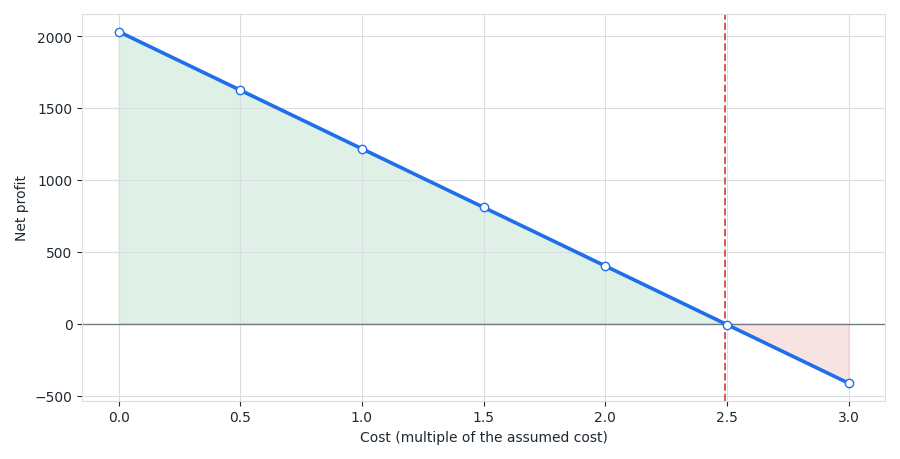
Fig. 2. The cost-sensitivity curve: net profit as the assumed cost is scaled up. The crossing point is the cushion.

Architecture of the Execution Cost Sensitivity Analyzer

The solution is a single MQL5 script organized into three modules, supported by one helper script:

1. Trade Loader: reads the per-deal result and volume from a CSV file. It is also provided as the standalone script CostLoader.mq5.
2. Cost Engine: re-prices the deals under a cost multiplier and computes the breakeven, the cushion, the figures at the assumed cost, and the win erosion. It is also provided as the standalone script CostEngine.mq5.
3. Scoring: combines the three dimensions into a weighted score and a grade, then prints recommendations. It is also provided as the standalone script CostScore.mq5.

The main script (CostSens.mq5) assembles the modules into one report. The helper (ExportCost.mq5) exports the input file from a backtest. We will build each module in turn and then assemble them. The analyzer expects a CSV file with one row per closing deal and up to three columns: date, deal result, and volume (lots). A deal closed in a single exit is one row; a position closed in several partial exits appears as several rows, and each exit pays its own cost.

The data model. We begin with the script properties, the inputs, and the structure that holds the report. Every figure the analyzer prints lives in one structure, and the cost model and the scoring are driven entirely by inputs, so nothing is hidden in a constant.

//--- Input parameters
input string InpFileName      = "Trades.csv"; // CSV file: Date,Profit,Volume (one row per closing deal)
input double InpCostPerLot    = 12.0;         // Assumed round-turn cost per 1.0 lot (spread + commission + slippage)
input double InpCostFixed     = 0.0;          // Assumed fixed cost per deal (e.g. minimum commission), account currency
input double InpCushionTarget = 3.0;          // Cushion (x assumed cost) that scores full marks on the cushion dimension
input double InpThinMult      = 1.0;          // A winner is "thin" if its result <= InpThinMult x its assumed cost
input double InpErosionTol    = 0.20;         // Win-erosion tolerance: this fraction of winners erased scores zero
input double InpWeightCushion = 0.45;         // Weight: cost-cushion dimension
input double InpWeightPF       = 0.30;        // Weight: profit-factor resilience dimension
input double InpWeightErosion  = 0.25;        // Weight: win-erosion dimension

//--- Aggregated report: every figure the analyzer prints lives here
struct SReport
  {
   int    nTrades;                            // total closing deals loaded from the file
   int    nWinners;                           // deals with a positive result, before cost
   int    nLosers;                            // deals with a negative result, before cost
   int    nFlat;                              // deals with exactly zero result
   double grossProfit;                        // sum of the winning deals, before cost
   double grossLoss;                          // sum of the losing deals, before cost, as a positive number
   double netProfit;                          // gross profit minus gross loss, before cost
   double profitFactor;                       // gross profit / gross loss; -1.0 means undefined (no losing deals)
   double winRate;                            // winners as a percentage of all deals
   double sumVol;                             // total traded volume across all deals (lots)
   double avgEdge;                            // net profit per deal (net / nTrades)
   double assumedCost;                        // total assumed cost across all deals (the C1 baseline)
   double avgCost;                            // assumed cost per deal (assumedCost / nTrades)
   double breakeven;                          // breakeven cost per deal that zeroes the net (equals avgEdge)
   double cushion;                            // breakeven multiplier: the net reaches zero at cushion x the assumed cost
   double netAtCost;                          // net profit left at the assumed cost level
   double pfAtCost;                           // profit factor at the assumed cost; -1.0 means no losing deals left
   double retention;                          // netAtCost / netProfit (0..1)
   int    erased;                             // winners that turn into non-winners at the assumed cost
   double erosionRate;                        // erased / nWinners (0..1)
   double thinShare;                          // share of gross profit from winners within InpThinMult x their cost
   double cushionScore;                       // cost-cushion dimension of the score, 0..100
   double pfScore;                            // profit-factor resilience dimension of the score, 0..100
   double erosionScore;                       // win-erosion dimension of the score, 0..100
   double composite;                          // weighted composite score, 0..100
   string grade;                              // letter grade from A+ to F
  };

//--- Globals
double g_profit[];                            // result of each loaded closing deal
double g_vol[];                               // volume (lots) of each loaded closing deal
string g_date[];                              // date of each loaded closing deal
int    g_n = 0;                               // number of deals currently loaded

Module 1: The Trade Loader. The loader opens the file as text, skips the header, and splits each row on the comma into a date, a result, and an optional volume. Reading as text and splitting on the delimiter tolerates blank lines and stray spaces better than reading field by field. When the volume column is missing or non-positive, it defaults to 1.0, so a plain two-column file of date and profit still works, with the cost then applied per deal rather than per lot.

//+------------------------------------------------------------------+
//| Read a Date,Profit,Volume file (one row per closing deal)        |
//| Read as text and split each row on the comma, which tolerates    |
//| blank lines and stray spaces better than field-by-field reading. |
//| The Volume column is optional: a missing or non-positive value   |
//| defaults to 1.0, so a plain Date,Profit file also works.         |
//+------------------------------------------------------------------+
bool LoadTrades(string filename, double &profit[], double &vol[], string &dates[])
  {
   int handle = FileOpen(filename, FILE_READ|FILE_TXT|FILE_ANSI);
   if(handle == INVALID_HANDLE)
     {
      PrintFormat("Could not open %s. Error: %d", filename, GetLastError());
      return false;
     }

   int  count = 0;
   bool firstLine = true;
   while(!FileIsEnding(handle))
     {
      //--- In FILE_TXT mode, FileReadString returns one line; trim its whitespace
      string row = FileReadString(handle);
      StringTrimLeft(row);
      StringTrimRight(row);
      if(firstLine)                   // the first line is the header
        {
         firstLine = false;
         continue;
        }
      if(row == "")                   // skip blank lines
         continue;

      //--- Split "Date,Profit,Volume" into its fields
      string parts[];
      if(StringSplit(row, ',', parts) < 2)
         continue;                    // need at least a date and a result
      StringTrimLeft(parts[0]);
      StringTrimRight(parts[0]);
      if(StringToTime(parts[0]) <= 0) // skip rows whose date does not parse
         continue;

      //--- The volume is optional; default to 1.0 when absent or non-positive
      double v = 1.0;
      if(ArraySize(parts) >= 3)
        {
         double parsed = StringToDouble(parts[2]);
         if(parsed > 0.0)
            v = parsed;
        }

      //--- Store the parsed deal
      count++;
      ArrayResize(profit, count, 512);
      ArrayResize(vol,    count, 512);
      ArrayResize(dates,  count, 512);
      profit[count - 1] = StringToDouble(parts[1]);
      vol[count - 1]    = v;
      dates[count - 1]  = parts[0];
     }

   FileClose(handle);
   return (count > 0);
  }

So that the script produces output on the first run, it generates a reproducible sample when no file is present. The seed is fixed, and the set is shaped to land on a believable middle grade rather than a perfect pass, with a few large winners, a band of ordinary winners and losers, and a handful of thin winners that costs can erase.

//+------------------------------------------------------------------+
//| Create a synthetic per-deal file when none is present            |
//+------------------------------------------------------------------+
bool EnsureSampleFile(string filename)
  {
   int handle = FileOpen(filename, FILE_WRITE|FILE_TXT|FILE_ANSI);
   if(handle == INVALID_HANDLE)
     {
      PrintFormat("Could not create sample %s. Error: %d", filename, GetLastError());
      return false;
     }

   FileWriteString(handle, "Date,Profit,Volume\n");
   MathSrand(20260601);                                               // fixed seed: the demo is reproducible

   int      trades    = 200;
   datetime t         = StringToTime("2026.01.05");
   int      todayLeft = 1 + (int)(MathRand() % 3);                    // 1-3 deals on the first day
   int      bigIdx[]  = {17, 53, 96, 134, 178};                       // a few large winners, spread out
   int      thinIdx[] = {8, 27, 49, 70, 88, 110, 129, 150, 171, 190}; // small winners costs can erase

   for(int i = 0; i < trades; i++)
     {
      //--- Volume first, so the call order stays stable across branches
      double vol = 0.10 + (MathRand() % 6) * 0.10;                    // 0.10..0.60 lots

      //--- Decide what kind of deal this is
      bool isBig = false, isThin = false;
      for(int b = 0; b < ArraySize(bigIdx); b++)
         if(bigIdx[b] == i)
           {
            isBig = true;
            break;
           }
      if(!isBig)
         for(int b = 0; b < ArraySize(thinIdx); b++)
            if(thinIdx[b] == i)
              {
               isThin = true;
               break;
              }

      double profit;
      if(isBig)
         profit = 110.0 + (i % 4) * 25.0;                             // engineered large winner
      else if(isThin)
         profit = 1.0 + (MathRand() % 5);                             // small winner the cost can erase
      else
        {
         double u = (double)MathRand() / 32767.0;
         if(u < 0.58)
            profit = 15.0 + (double)MathRand() / 32767.0 * 66.0;      // ordinary winner
         else
            profit = -(20.0 + (double)MathRand() / 32767.0 * 52.0);   // loser
        }

      //--- Write the row and advance the calendar by 1-3 deals per day
      MqlDateTime dt;
      TimeToStruct(t, dt);
      string ds = StringFormat("%04d.%02d.%02d", dt.year, dt.mon, dt.day);
      FileWriteString(handle, StringFormat("%s,%.2f,%.2f\n", ds, profit, vol));

      todayLeft--;
      if(todayLeft <= 0)
        {
         t += 86400;
         todayLeft = 1 + (int)(MathRand() % 3);
        }
     }

   FileClose(handle);
   PrintFormat("Sample file %s created with %d deals.", filename, trades);
   return true;
  }

Module 2: The Cost Engine. The engine is the analytical core. Its central routine re-prices every deal at a chosen multiple of the assumed cost and returns the net profit, writing the profit factor through a reference parameter. Calling it at a multiplier of zero gives the figures before any added cost; calling it at 1.0 gives the figures at the assumed cost; sweeping the multiplier traces the cost-sensitivity curve.

//+------------------------------------------------------------------+
//| Net profit and profit factor at a cost multiplier                |
//| Each deal pays mult x (InpCostFixed + InpCostPerLot x volume).   |
//| Returns the net after cost; writes the profit factor to pfOut    |
//| (-1.0 when no losing deals remain after the cost is applied).    |
//+------------------------------------------------------------------+
double NetAtMultiplier(const double &profit[], const double &vol[], int n, double mult, double &pfOut)
  {
   double gp = 0.0, gl = 0.0;
   for(int i = 0; i < n; i++)
     {
      double cost = mult * (InpCostFixed + InpCostPerLot * vol[i]); // cost charged to this deal
      double net  = profit[i] - cost;
      if(net > 0.0)
         gp += net;                                                 // still a winner after cost
      else if(net < 0.0)
         gl += -net;                                                // a loser after cost
     }
   pfOut = (gl > 0.0) ? gp / gl : -1.0;                             // -1 means no losing deals remain
   return gp - gl;
  }

A profit factor of -1.0 is a deliberate sentinel: it marks the case where no losing deals remain, so the ratio is undefined rather than zero or infinity. The second routine counts the winners that a given cost erases, which feeds both the win-erosion figure and one of the scoring dimensions.

//+------------------------------------------------------------------+
//| Count the winners erased at a given cost multiplier              |
//+------------------------------------------------------------------+
int CountErased(const double &profit[], const double &vol[], int n, double mult)
  {
   int erased = 0;
   for(int i = 0; i < n; i++)
     {
      if(profit[i] <= 0.0) // only winners can be erased
         continue;
      double cost = mult * (InpCostFixed + InpCostPerLot * vol[i]);
      if(profit[i] - cost <= 0.0)
         erased++;
     }
   return erased;
  }

Module 3: Scoring. The scoring module combines three dimensions into a single score. The cushion dimension measures the margin over the assumed cost, with full marks at the configurable target and zero at breakeven. The profit-factor resilience dimension measures how much of the edge above 1.0 survives the assumed cost. The win-erosion dimension penalizes winners that turn into losers once the cost is applied. The weights are normalized by their sum, so the result does not depend on whether they add up to one. The composite maps to a grade from A+ to F. The score is a heuristic for ranking and quick comparison under one set of cost assumptions, not an industry-standard metric.

//+------------------------------------------------------------------+
//| Map the three dimensions to a weighted score and a letter grade  |
//| cushion        : net reaches zero at (cushion) x the assumed cost|
//| pfBefore/pfCost: profit factor before and at the assumed cost    |
//| erosionRate    : fraction of winners erased at the assumed cost  |
//+------------------------------------------------------------------+
double ScoreReport(double cushion, double pfBefore, double pfCost, double erosionRate, string &grade)
  {
   //--- Cushion dimension: full marks at InpCushionTarget, zero at breakeven (1x)
   double ct = MathMax(1.0001, InpCushionTarget); // guard the denominator
   double cushionScore = MathMax(0.0, MathMin(100.0, 100.0 * (cushion - 1.0) / (ct - 1.0)));

   //--- Profit-factor resilience dimension: how much of the edge above 1.0 survives the cost
   double pfScore;
   if(pfBefore < 0.0)                             // no losers at all: fully resilient
      pfScore = 100.0;
   else if(pfBefore <= 1.0)                       // not profitable even before cost
      pfScore = 0.0;
   else if(pfCost < 0.0)                          // no losers left after cost
      pfScore = 100.0;
   else
      pfScore = MathMax(0.0, MathMin(100.0, 100.0 * (pfCost - 1.0) / (pfBefore - 1.0)));

   //--- Win-erosion dimension: penalize winners that the cost turns into losers
   double et = MathMax(0.0001, InpErosionTol);    // guard the denominator
   double erosionScore = MathMax(0.0, MathMin(100.0, 100.0 * (1.0 - erosionRate / et)));

   //--- Normalize the weights so the result does not depend on their sum
   double wc = MathMax(0.0, InpWeightCushion);
   double wp = MathMax(0.0, InpWeightPF);
   double we = MathMax(0.0, InpWeightErosion);
   double wsum = wc + wp + we;
   if(wsum <= 0.0)
     {
      wc = 0.45; wp = 0.30; we = 0.25; wsum = 1.0;
      Print("Warning: weights were non-positive; reverting to the 0.45 / 0.30 / 0.25 default.");
     }
   wc /= wsum; wp /= wsum; we /= wsum;

   //--- Composite score and its letter grade
   double composite = cushionScore * wc + pfScore * wp + erosionScore * we;
   PrintFormat("  Cushion score:  %.1f / 100", cushionScore);
   PrintFormat("  PF-resilience:  %.1f / 100", pfScore);
   PrintFormat("  Win-erosion:    %.1f / 100", erosionScore);

   if(composite >= 90)      grade = "A+";
   else if(composite >= 80) grade = "A";
   else if(composite >= 70) grade = "B";
   else if(composite >= 60) grade = "C";
   else if(composite >= 50) grade = "D";
   else                     grade = "F";
   return composite;
  }

The Main Script: Putting It All Together

The main script wires the modules into one report. It loads deals (or builds a sample), validates the dataset, and prints the summary, cost-sensitivity curve, sensitivity metrics, score, and recommendations. Each recommendation is driven by a specific weakness, so the advice changes with the data rather than repeating a fixed list.

//+------------------------------------------------------------------+
//| Script entry point                                               |
//+------------------------------------------------------------------+
void OnStart()
  {
   Print("========================================");
   Print("  EXECUTION COST SENSITIVITY ANALYZER v1.0");
   Print("  How much execution cost can the edge absorb?");
   Print("========================================");

   //--- Load the deals, or build and load a sample set if none is found
   if(!LoadTrades(InpFileName, g_profit, g_vol, g_date))
     {
      Print(">> File not found or empty. Generating a sample set...");
      if(!EnsureSampleFile(InpFileName))
        {
         Alert("Could not create the sample file.");
         return;
        }
      if(!LoadTrades(InpFileName, g_profit, g_vol, g_date))
        {
         Alert("Could not load the sample file.");
         return;
        }
     }

   g_n = ArraySize(g_profit);
   if(g_n < 20)           // too few deals for the figures to be meaningful
     {
      Alert("At least 20 deals are required (results are more reliable with 100+).");
      return;
     }

   SReport r;
   BuildReport(g_profit, g_vol, g_n, r);

   Print("\nNote: this works at the closing-deal level. A position closed in several");
   Print("deals (partial exits) is several rows, and each exit deal pays its own cost.");

   if(r.netProfit <= 0.0) // the analysis needs a profitable set to make sense
     {
      Print("\nNet profit is not positive before cost; the cost analysis needs a profitable set.");
      PrintFormat("Net: %.2f | Deals: %d", r.netProfit, r.nTrades);
      return;
     }

   //--- Headline figures
   Print("\n=== STRATEGY (before added cost) ===");
   PrintFormat("  Deals:           %d  (%d winners, %d losers, %d flat)", r.nTrades, r.nWinners, r.nLosers, r.nFlat);
   PrintFormat("  Win rate:        %.1f%%", r.winRate);
   PrintFormat("  Net profit:      %.2f", r.netProfit);
   PrintProfitFactor("  Profit factor:   ", r.profitFactor);
   PrintFormat("  Total volume:    %.2f lots  (avg %.2f per deal)", r.sumVol, AvgVolume(g_vol, g_n));
   PrintFormat("  Edge per deal:   %.2f", r.avgEdge);

   //--- The assumed cost and the cost curve
   PrintFormat("\n=== ASSUMED COST: %.2f per lot + %.2f fixed (%.2f per deal on average) ===",
               InpCostPerLot, InpCostFixed, r.avgCost);
   Print("");
   PrintCostCurve(g_profit, g_vol, g_n, r.netProfit);

   //--- The cost sensitivity results
   Print("\n=== COST SENSITIVITY ===");
   PrintFormat("  Breakeven cost per deal: %.2f  (the edge per deal)", r.breakeven);
   PrintFormat("  Cushion:                 %.2fx the assumed cost", r.cushion);
   PrintFormat("  Net at the assumed cost: %.2f  (%.0f%% of the original net)", r.netAtCost, r.retention * 100.0);
   PrintProfitFactor("  Profit factor at cost:   ", r.pfAtCost);
   PrintFormat("  Winners erased at cost:  %d of %d  (%.1f%%)", r.erased, r.nWinners, r.erosionRate * 100.0);
   PrintFormat("  Thin-winner gross share: %.1f%%", r.thinShare);
   Print("  (One-sided: only cost rises, so the net and the profit factor are meant to fall.)");

   //--- Score
   Print("\n========================================");
   Print("  COST-ROBUSTNESS SCORE (heuristic)");
   Print("========================================");
   PrintFormat("  Cushion score:    %.1f / 100", r.cushionScore);
   PrintFormat("  PF-resilience:    %.1f / 100", r.pfScore);
   PrintFormat("  Win-erosion:      %.1f / 100", r.erosionScore);
   Print("----------------------------------------");
   PrintFormat("  COMPOSITE:        %.1f / 100", r.composite);
   PrintFormat("  GRADE:            %s", r.grade);
   Print(" (Heuristic for ranking and quick comparison, not a statistically validated measure.)");
   Print("========================================");

   //--- Recommendations: each one is driven by a specific weakness
   Print("\n--- RECOMMENDATIONS ---");
   if(r.cushion < 2.0)
      PrintFormat("!! The edge disappears below 2x the assumed cost (cushion %.2fx). Treat live results with great caution.", r.cushion);
   else if(r.cushion < 3.0)
      PrintFormat(">> The cushion is only %.2fx the assumed cost. A modest rise in spread or slippage materially cuts the result; build in margin before trading live.", r.cushion);
   if(r.profitFactor > 0.0 && r.pfAtCost > 0.0 && r.pfAtCost < 1.4)
      PrintFormat(">> At the assumed cost the profit factor falls to %.2f. The edge is thin once realistic costs are paid.", r.pfAtCost);
   if(r.retention < 0.70)
      PrintFormat(">> Realistic costs erase %.0f%% of the net profit (%.2f -> %.2f).", (1.0 - r.retention) * 100.0, r.netProfit, r.netAtCost);
   if(r.erosionRate >= 0.10)
      PrintFormat(">> %.0f%% of winning deals turn into losers at the assumed cost. The result leans on marginal winners.", r.erosionRate * 100.0);
   if(r.cushion >= 3.0 && r.pfAtCost >= 1.5)
      Print("++ The edge absorbs several times the assumed cost and keeps a healthy profit factor. It looks robust to execution costs.");

   Print("\nAnalysis complete.");
  }

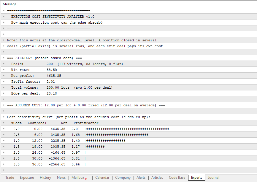
Fig. 3. The full report for the sample set is shown in the Experts tab.

Exporting Your Own Trades

To analyze a real strategy, you need its closing deals in the same format: date, profit, and volume. The helper reads the account or tester history, keeps only the buy and sell deals that close a position, and writes one row per closing deal. By default it exports the price result only, excluding the commission and swap already charged, so the analyzer can model the full execution cost on top without counting it twice. If you prefer to fold the charged fees back in, set the InpIncludeFees input. A clean approach is to set backtest commission to zero, export gross results, and let the tool apply realistic costs on top.

//+------------------------------------------------------------------+
//| Write one row per closing deal: its result and its volume        |
//+------------------------------------------------------------------+
void ExportCost(string filename)
  {
   //--- Open the output file and write the header
   int handle = FileOpen(filename, FILE_WRITE|FILE_TXT|FILE_ANSI);
   if(handle == INVALID_HANDLE)
     {
      PrintFormat("Cannot create %s. Error: %d", filename, GetLastError());
      return;
     }
   FileWriteString(handle, "Date,Profit,Volume\n");

   //--- Pull the whole trade history into the cache
   if(!HistorySelect(0, TimeCurrent()))
     {
      Print("HistorySelect failed.");
      FileClose(handle);
      return;
     }

   int total = HistoryDealsTotal();
   int rows  = 0;

   for(int i = 0; i < total; i++)
     {
      ulong ticket = HistoryDealGetTicket(i);
      if(ticket == 0)
         continue;

      //--- Keep only real trade deals (buy/sell). This excludes balance,
      //--- credit, charge, correction, bonus, interest and similar entries.
      ENUM_DEAL_TYPE dtype = (ENUM_DEAL_TYPE)HistoryDealGetInteger(ticket, DEAL_TYPE);
      if(dtype != DEAL_TYPE_BUY && dtype != DEAL_TYPE_SELL)
         continue;

      //--- Only closing deals carry a trade's realized result. A partial
      //--- or multi-deal exit yields several closing deals, so one
      //--- position can contribute more than one row.
      if((ENUM_DEAL_ENTRY)HistoryDealGetInteger(ticket, DEAL_ENTRY) != DEAL_ENTRY_OUT)
         continue;

      //--- The price result of the deal. By default commission and swap are
      //--- excluded, so the analyzer can add the modeled cost without double
      //--- counting; set InpIncludeFees to fold the charged fees back in.
      double profit = HistoryDealGetDouble(ticket, DEAL_PROFIT);
      if(InpIncludeFees)
         profit += HistoryDealGetDouble(ticket, DEAL_SWAP)
                 + HistoryDealGetDouble(ticket, DEAL_COMMISSION);

      //--- The deal volume in lots, used to scale the per-lot cost
      double volume = HistoryDealGetDouble(ticket, DEAL_VOLUME);

      //--- Write the row as Date,Profit,Volume (the date is the close time)
      datetime dealTime = (datetime)HistoryDealGetInteger(ticket, DEAL_TIME);
      MqlDateTime dt;
      TimeToStruct(dealTime, dt);
      FileWriteString(handle, StringFormat("%04d.%02d.%02d,%.2f,%.2f\n", dt.year, dt.mon, dt.day, profit, volume));
      rows++;
     }

   FileClose(handle);
   PrintFormat("Exported %d closing deals to %s", rows, filename);
  }

Interpreting the Results

Run the script with no input file, and it analyzes the built-in sample of 200 deals. The strategy looks tradeable before cost: a net profit of 2031.14, a profit factor of 1.56, and a win rate of 61.0%, on a total of 67.90 lots. The edge per deal is 10.16, so the breakeven cost per deal is also 10.16.

Now apply the assumed cost of 12 units per lot. The average deal trades about 0.34 lots, the assumed cost averages 4.07 per deal, and the cushion works out to 2.49. In other words, the edge survives execution costs up to about two and a half times what we assumed, and no further. At the assumed cost, the net profit falls to 1216.34, which is 60% of the original; the other 40% is paid away. The profit factor drops from 1.56 to 1.31, and 6 of the 122 winners turn into losers. The composite score is 69.0, a grade of C.

The recommendations follow from those numbers. The cushion is below 3.0, so the tool warns that a modest rise in spread or slippage materially cuts the result. The profit factor at cost is below 1.4, so it flags that the edge is thin once realistic costs are paid. And because realistic costs erase 40% of the net profit, it says so plainly. The reading is clear: this strategy is not worthless, but it is cost-sensitive, and it needs a margin of safety, a cheaper broker, or fewer and larger trades before it goes live.

The same workflow ranks candidates. Run two strategies through the analyzer with the same assumed cost, and the one with the higher cushion is the one more likely to keep its edge on a real account. A cushion above 3.0 with a profit factor that stays healthy at cost earns the positive note and is the kind of result worth trading.

Applicability and Limitations

The analyzer is a planning tool, not a guarantee. It needs a reasonable sample to be meaningful; below about 100 deals, the figures move too much from a single large trade, and the script refuses to run below 20. It works at the closing-deal level, the granularity MetaTrader 5 records, so a position closed in several partial exits is several rows, and the modeled cost is charged to each exit, which matches how a broker bills.

The cost model is intentionally simple: a fixed part plus a linear per-lot part, applied equally to every deal. Real slippage is not constant; it is worse in fast markets and around news, and it can depend on order type and size. Treat the assumed cost as a considered estimate and read the cushion as the margin over it, not as a promise that the cost will never exceed it. The cushion and the breakeven are exact for the linear model; the profit factor at cost and the win erosion depend on the distribution of your deals.

Finally, cost robustness is one dimension among several. It complements, rather than replaces, walk-forward testing, which checks that the edge persists out of sample, and Monte Carlo resampling, which checks how sensitive the result is to the order of trades. A strategy worth trading should pass all three: a stable edge, a tolerable spread of outcomes, and a comfortable margin over costs.

Conclusion

We set out to answer a question that headline metrics hide: how much execution cost can the edge absorb? The analyzer answers it directly. It reads a record of closing deals, finds the breakeven cost per deal, measures the cushion over a realistic assumed cost, re-prices the whole record to show the net profit and profit factor at that cost, counts the winners the cost erases, and folds the three dimensions into a graded score with concrete advice. The sample strategy earned a C: profitable on paper, but with only a 2.49x cushion and 40% of its net profit lost to realistic costs.

All source files are attached and compile natively in MetaEditor, so a reader can run the analyzer on their own trades, see how close the edge sits to the cost line, and decide whether it is ready for a live account. The source code is available in the MQL5 CodeBase: Execution Cost Sensitivity Analyzer in the MQL5 CodeBase.

The following table describes the source files that accompany the article.

File Name	Description
CostSens	The main script. It loads the deals, runs the engine and the scoring, and prints the full cost-robustness report with the cost curve.
CostLoader	Module 1 reads the input file (date, profit, and volume) and prints a quick summary for verification.
CostEngine	Module 2 re-prices the deals under a rising cost and computes the breakeven, the cushion, and the win erosion.
CostScore	Module 3 combines the three dimensions into a graded score and prints the recommendations.
ExportCost	A helper that exports a file of date, profit, and volume from the trade history. Copy its function into your Expert Advisor and call it from OnTester, or run it as a script.
MQL5.zip	An archive whose root is the MQL5 folder, so it unpacks directly into the terminal data folder with every file in its correct place. The five scripts sit in MQL5\Scripts\CostSens\, ready to compile without moving anything.

References:

1. MetaQuotes, "MQL5 Reference: File Functions," MQL5 Documentation: Files
2. MetaQuotes, "MQL5 Reference: Trade History," MQL5 Documentation: HistoryDealGetDouble
3. MetaQuotes, "Guidelines for writing articles: screenshots," How to Write an Article
4. Execution Cost Sensitivity Analyzer source code, MQL5 CodeBase: Execution Cost Sensitivity Analyzer in the MQL5 CodeBase