Multi-Threaded Trading Robot with Machine Learning: From Concept to Implementation

This project is a revival of one of my old codes. The code has been sitting on dusty hard drives for years, and by now it no longer runs: too much has changed in the development environment. I decided not only to revive the development, but also to explain it step by step over the course of several articles.

The original idea was to develop a multi-threaded robot using powerful parallel computing, possibly even using cloud computing clusters. Imagine this: you are sitting in front of multiple monitors, watching currency pairs move, and you realize the human brain is simply not capable of simultaneously monitoring dozens of instruments, analyzing hundreds of indicators, and making decisions at the speed required by modern markets. It was at this point that the idea of creating an intelligent trading robot was born, capable of working with a portfolio of instruments and analyzing decades of data in parallel.

But why Python and not the built-in MQL5? This question probably arises in the minds of everyone who sees the hybrid architecture of our solution. The answer lies in the nature of the problems we solve. Machine learning requires powerful libraries like scikit-learn, XGBoost, and pandas — an ecosystem that seems tailor-made for such tasks.

Another reason for this choice: the architecture of our robot is built on the philosophy of division of responsibility and division of labor. Python is responsible for the "brains" - data collection, pre-processing, feature creation, model training, and trading signal generation. MetaTrader 5, through its Python API, acts as the "hands" — executing orders, managing positions, and providing real-time market data.

Multithreading is becoming not just a technical solution, but a necessity. When your robot has to analyze EURUSD, GBPUSD, AUDUSD and other pairs at the same time, sequential processing becomes a bottleneck. Each thread receives its own currency pair, its own model and its own decision-making context. It is similar to how experienced traders can hold multiple trading ideas in their heads at the same time, but with the computing power of a machine.

A distinctive feature of our approach is the integration of risk management at the portfolio level. Instead of each instrument being traded independently, we introduce the TOTAL_PORTFOLIO_RISK global variable that limits the total risk of the portfolio. This means that the position size for each instrument is calculated not only based on its volatility, but also taking into account already open positions on other instruments.

TOTAL_PORTFOLIO_RISK: float = 500.0
POSITION_SIZES: Dict[str, float] = {}
SYMBOL_TRADES: Dict[str, bool] = {}

Logging system and market data retrieval

Before we dive into machine learning algorithms, we need to build a solid foundation — a logging and data retrieval system. Have you ever tried to debug a multithreaded application without logs? It is like looking for a needle in a haystack blindfolded.

Our logging system is built around a queue with a limited size — a solution that may seem overly complex, but has profound implications. Imagine the situation: five threads are simultaneously trying to write information to the console. Without coordination, you will end up with a mess of jumbled messages. The queue ensures consistency, and a separate printer thread ensures the readability of the logs.

log_queue = queue.Queue(maxsize=1000)

def log_printer():
    while True:
        try:
            log_message = log_queue.get(timeout=10)
            if log_message is None:
                break
            print(log_message)
        except queue.Empty:
            continue

Why exactly 1000 messages in the queue? This is the result of practical experience. A queue that is too small will result in the loss of important messages during periods of high activity, while a queue that is too large will result in excessive memory consumption. 1000 messages is the optimal balance for a trading robot.

Now we move on to the heart of our system - the retrieve_data function. It seems simple, but it contains a philosophy of reliability. Look at the variable retries_limit = 300. This is not a random number. In real trading, brokerage servers may be unavailable for seconds, sometimes minutes. 300 attempts at one-second intervals gives us a 5-minute recovery window.

Particular attention is paid to the creation of technical indicators. We do not just calculate RSI or MACD - we create an entire ecosystem of interconnected features. RSI shows whether an asset is overbought or oversold. MACD reveals changes in momentum. ATR measures volatility. But the magic happens when these indicators interact within a machine learning model.

# RSI (Relative Strength Index)
delta = raw_data['close'].diff()
gain = delta.where(delta > 0, 0).rolling(14).mean()
loss = (-delta.where(delta < 0, 0)).rolling(14).mean()
rs = gain / loss
raw_data['RSI_14'] = (100 - (100 / (1 + rs))).astype(np.float64)

Note that we use np.float64 instead of float32. This seems like a waste of memory, but later functions require high precision calculations. Saving on accuracy can lead to instability of feature clustering.

Each technical indicator has its own "personality". Williams %R reacts aggressively to price changes. Aroon Oscillator shows the strength of the trend. Efficiency Ratio measures the "purity" of price movement. When all of these indicators are combined into machine learning models, they create a multidimensional view of the market that is beyond human perception.

Data augmentation and creation of synthetic samples

Machine learning is hungry for data, but financial markets are stingy with historical examples. How to solve this dilemma? Data augmentation becomes our key to creating a rich training set from a limited history.

The augment_data function implements four data augmentation strategies, each with a deep rationale. The first strategy is to add noise. You may ask: why spoil clean data? The answer lies in the nature of real markets. Prices never move perfectly smoothly — there are always microfluctuations, slippage, and random spikes. By adding controlled noise, we prepare the model for real-world conditions.

noisy_data = raw_data.astype(np.float32) + np.random.normal(0, noise_level, raw_data.shape).astype(np.float32)

The parameter noise_level = 0.01 was not chosen by chance. This is approximately 1% of the feature value — enough to create variability, but not so much as to distort patterns. Think of it as a gentle ripple on the water, it does not change the direction of the flow, but it adds realism.

The second strategy is time shifting. We create a copy of the data shifted forward by one hour. It may seem artificial, but financial patterns often repeat themselves with slight time shifts. Morning volatility may reappear in the evening, and weekly cycles may shift by a day or two.

The third strategy is scaling. We multiply all values by a random coefficient from 0.9 to 1.1. This simulates different market conditions: periods of high and low volatility, bull and bear markets. A model trained on only one period of data may be helpless when market conditions change.

The fourth strategy is the inversion of price columns. We multiply the price data by -1, effectively turning the chart upside down. This trains the model to recognize mirror patterns. When inverted, the head and shoulders pattern becomes a reverse head and shoulders, but the mathematical relationships between the features are preserved.

for col in price_columns:
    if col in inverted_data.columns:
        inverted_data[col] *= -1

It is critically important to process the results of augmentation correctly. Floating-point operations can produce infinite values, or NaN. Our cleaning strategy uses medians to fill in problematic values—a more robust approach than means, which can be skewed by outliers.

After augmentation, the data volume increases fivefold. From 1000 historical hours we get 5000 training examples. But this is not just a quantitative increase - it is a qualitative enrichment. The model sees not only what was, but also options for what could have been under slightly different conditions.

We pay special attention to processing trading volume. Unlike prices, volume cannot be negative, so we leave it alone when inverting, and when adding noise, we truncate it below by zero. This supports the economic logic of the data.

Data labeling and creation of target variables

Machine learning without properly labeled data is like trying to teach a child to read by showing them letters without explaining their meaning. The markup_data and label_data functions solve the fundamental problem of turning raw price data into training examples with clear target labels.

The markup_data function implements the simplest labeling approach: it predicts whether the price in one period will be higher than the current price by the markup_ratio value. This approach seems primitive, but its simplicity is deceptive. The markup_ratio parameter = 0.00002 (2 pips for most currency pairs) takes into account real trading costs.

def markup_data(
    data: pd.DataFrame,
    target_column: str,
    label_column: str,
    markup_ratio: float = 0.00002
) -> pd.DataFrame:
    log("Starting markup_data function")
    data[label_column] = np.where(
        data[target_column].shift(-1) > data[target_column] + markup_ratio,
        1,
        0
    ).astype(np.int8)
    data.loc[data[label_column].isna(), label_column] = 0
    log(f"Number of labels set for price change greater than markup ratio: {data[label_column].sum()}")
    return data

The label_data function represents a more sophisticated approach. Instead of simply comparing prices over one period, it simulates a real trading strategy with stop losses and take profits. This is critically important because financial markets are nonlinear. The price may reach your target, but touch your stop loss on the way.

def label_data(
    data: pd.DataFrame,
    symbol: str,
    min_days: int = 2,
    max_days: int = 72
) -> pd.DataFrame:
    if not mt5.initialize(path=TERMINAL_PATH):
        log("Terminal connection error")
        return data

    symbol_info = mt5.symbol_info(symbol)
    stop_level: float = 300 * symbol_info.point
    take_level: float = 800 * symbol_info.point
    labels: List[Optional[int]] = []

    for i in range(data.shape[0] - max_days):
        rand: int = random.randint(min_days, max_days)
        curr_pr: float = data['close'].iloc[i]
        future_pr: float = data['close'].iloc[i + rand]
        min_pr: float = data['low'].iloc[i:i + rand].min()
        max_pr: float = data['high'].iloc[i:i + rand].max()
        price_change: float = abs(future_pr - curr_pr)

        if (price_change > take_level and
            future_pr > curr_pr and
            min_pr > curr_pr - stop_level):
            labels.append(1)
        elif (price_change > take_level and
              future_pr < curr_pr and
              max_pr < curr_pr + stop_level):
            labels.append(0)
        else:
            labels.append(None)

The labeling algorithm works as follows: for each time point, we select a random horizon from min_days to max_days (from 2 to 72 hours). Then we analyze the price behavior in this interval. The logic of checking is three-level: is the price movement large enough (price_change > take_level), is the direction correct (future_pr > curr_pr for purchases), and was the stop-loss not triggered prematurely (min_pr > curr_pr - stop_level).

Why random time horizons? This prevents the model from overfitting to fixed time intervals. Markets are unaware of our analysis periods - a pattern can develop in 5 hours or in 50. Randomness makes the model more adaptive to different time scales of market movements.

data = data.iloc[:len(labels)].copy()
    data['labels'] = labels
    data.dropna(inplace=True)

    X = data.drop('labels', axis=1)
    y = data['labels']

    rus = RandomUnderSampler(random_state=2)
    X_balanced, y_balanced = rus.fit_resample(X, y)

    data_balanced = pd.concat([X_balanced, y_balanced], axis=1)
    log(f"Number of growth labels (1.0): {data_balanced['labels'].value_counts().get(1.0, 0)}")
    log(f"Number of decline labels (0.0): {data_balanced['labels'].value_counts().get(0.0, 0)}")
    return data_balanced

The parameters stop_level = 300 points and take_level = 800 points set the risk/reward ratio to approximately 1:2.67. These values are multiplied by symbol_info.point, which automatically adapts them to the specific tool. For EURUSD with point = 0.00001 this corresponds to a 300-point stop loss and an 800-point take profit (roughly 30 and 80 pips, depending on the broker’s quote format).

RandomUnderSampler solves the problem of class imbalance radically - it removes random examples from the majority class until balance is achieved. In financial data, there are always more periods of "no clear signal" than clear trading opportunities. Without balancing, the model will learn to predict "no signal" in 90% of cases and will be formally accurate, but practically useless.

Feature generation and clustering with Gaussian Mixture Models

Once we have created a basic set of technical indicators, the question arises: how can we extract even more information from the available data? The generate_new_features function solves this problem by automatically generating derived features using random combinations of existing ones.

The philosophy behind this approach is simple but powerful: if two features individually contain useful information, then their mathematical combinations can reveal hidden patterns. Imagine that one indicator shows the strength of a trend, and another shows its sustainability. Their product can reveal moments when a strong trend becomes unsustainable.

def generate_new_features(
    data: pd.DataFrame,
    num_features: int = 10,
    random_seed: int = 1
) -> pd.DataFrame:
    random.seed(random_seed)
    new_features: Dict[str, pd.Series] = {}

    columns = data.columns
    for i in range(num_features):
        feature_name = f'feature_{i}'
        col1_idx, col2_idx = random.sample(range(len(columns)), 2)
        col1, col2 = columns[col1_idx], columns[col2_idx]
        operation = random.choice([
            'add', 'subtract', 'multiply', 'divide',
            'shift', 'rolling_mean', 'rolling_std',
            'rolling_max', 'rolling_min', 'rolling_sum'
        ])

The randomness in the choice of columns and operations may seem chaotic, but it provides variety. A deterministic approach might miss non-obvious but useful combinations. The division operation requires special care - we add a small value of 1e-8 to the denominator to avoid division by zero.

elif operation == 'divide':
            new_features[feature_name] = (data[col1] / (data[col2] + 1e-8)).astype(np.float32)
        elif operation == 'shift':
            shift = random.randint(1, 10)
            new_features[feature_name] = data[col1].shift(shift).fillna(method='ffill').fillna(method='bfill').astype(np.float32)

Shift operations create lagged features with random depth from 1 to 10 periods. This allows the model to "remember" the past at different time horizons. Moving statistics add smoothed versions of the original features, which can reveal long-term trends hidden in short-term noise.

The next step is feature clustering using Gaussian Mixture Models. This is one of the most elegant parts of our system. GMM assumes that the data is generated by a mixture of several normal distributions. In the context of financial markets, this means dividing into regimes - bull market, bear market, sideways movement, high volatility, low volatility.

def cluster_features_by_gmm(
    data: pd.DataFrame,
    n_components: int = 6
) -> pd.DataFrame:
    X = data.drop(['label', 'labels'], axis=1, errors='ignore').astype(np.float32)
    X = X.replace([np.inf, -np.inf], np.nan).fillna(X.median(numeric_only=True))

    gmm = GaussianMixture(
        n_components=n_components,
        covariance_type='full',
        reg_covar=0.1,
        random_state=1
    )
    gmm.fit(X)
    data['cluster'] = gmm.predict(X).astype(np.int16)
    return data

The n_components = 6 is chosen as a compromise between detail and interpretability. Too few clusters result in loss of nuance, too many result in overfitting and instability. Six clusters allow us to capture the main market regimes: strong bullish trend, weak bullish trend, low volatility sideways movement, high volatility sideways movement, weak bearish trend, strong bearish trend.

The covariance_type='full' parameter allows GMM to model correlations between features. This is critical in finance, where variables are rarely independent. RSI and MACD can behave differently under different market conditions, and the full covariance matrix takes this into account.

Covariance regularization (reg_covar=0.1) prevents model degeneracy in cases where the data are almost linearly dependent. In financial data, such situations arise regularly, for example when several indicators show extreme values at the same time.

Cluster affiliation becomes a new powerful feature. The machine learning model receives information not only about the specific values of the indicators, but also about the market regime the current situation belongs to. This adds contextual information that can dramatically change the interpretation of other features.

Recursive feature elimination and XGBoost learning with ensembling

With dozens of technical indicators, generated features, and cluster labels at our disposal, we are faced with the classic problem of the "curse of dimensionality." More features do not always mean a better model. Conversely, redundant and correlated features can lead to overfitting and reduced generalization ability.

The feature_engineering function solves this dilemma using recursive feature elimination with cross-validation (RFECV). This method works like an experienced trader who gradually eliminates unnecessary indicators from his arsenal, leaving only the most informative ones.

def feature_engineering(
    data: pd.DataFrame,
    n_features_to_select: int = 15
) -> pd.DataFrame:
    X = data.drop(['label', 'labels'], axis=1, errors='ignore').astype(np.float32)
    y = data['labels'].astype(np.int8)
    X = X.replace([np.inf, -np.inf], np.nan).fillna(X.median(numeric_only=True))

    unique_classes = y.unique()
    if len(unique_classes) < 2:
        log(f"Error in feature_engineering: Only one class found in labels: {unique_classes}")
        raise ValueError(f"The target 'y' needs to have more than 1 class. Got {len(unique_classes)} class instead")

    clf = RandomForestClassifier(n_estimators=100, random_state=1)
    rfecv = RFECV(
        estimator=clf,
        step=1,
        cv=5,
        scoring='accuracy',
        n_jobs=1,
        verbose=1,
        min_features_to_select=n_features_to_select
    )
    rfecv.fit(X, y)

RFECV works iteratively: it starts with all features, trains the model, determines the importance of each feature, removes the least important one, and repeats the process. step=1 means that at each iteration only one feature is removed - slowly but accurately. An alternative would be step=5 to speed things up, but in finance the cost of error is too high.

The choice of RandomForestClassifier as the base estimator is not accidental. Random forest works well with heterogeneous features and is robust to outliers. Its feature_importances_ are based on Gini impurity decay, which provides an intuitive importance metric.

selected_features = X.columns[rfecv.get_support()]
    selected_data = data[selected_features.tolist() + ['label', 'labels']]
    log("\nBest features:")
    log(str(pd.DataFrame({'Feature': selected_features})))
    return selected_data

Now let's move on to the heart of our system: XGBoost training with ensemble. XGBoost is renowned for its performance in financial problems due to its ability to model nonlinear interactions between features and its resistance to overfitting.

def train_xgboost_classifier(
    data: pd.DataFrame,
    num_boost_rounds: int = 500
) -> BaggingClassifier:
    if data.empty:
        raise ValueError("Data should not be empty")

    X = data.drop(['label', 'labels'], axis=1).astype(np.float32)
    y = data['labels'].astype(np.int8)

    clf = xgb.XGBClassifier(
        objective='binary:logistic',
        random_state=1,
        max_depth=5,
        learning_rate=0.2,
        n_estimators=300,
        subsample=0.01,
        colsample_bytree=0.1,
        reg_alpha=1,
        reg_lambda=1
    )

XGBoost parameters are selected for working with financial data: max_depth=5 limits the depth of the trees, preventing overfitting on noisy data; learning_rate=0.2 ensures sufficiently fast training while maintaining stability. The regularization parameters are critical: subsample=0.01 means that each tree is trained on only 1% of the data, which drastically reduces overfitting; colsample_bytree=0.1 indicates that each tree uses only 10% of the features. This may seem extreme, but when combined with a large number of trees (n_estimators=300), it creates a powerful ensemble of diverse weak learners.

bagging_clf = BaggingClassifier(estimator=clf, random_state=1)
    param_grid = {
        'n_estimators': [10, 20, 30],
        'max_samples': [0.5, 0.7, 1.0],
        'max_features': [0.5, 0.7, 1.0]
    }

    grid_search = GridSearchCV(bagging_clf, param_grid, cv=5, scoring='accuracy')
    grid_search.fit(X, y)
    accuracy = grid_search.best_score_
    log(f"Average cross-validation accuracy: {accuracy:.2f}")
    return grid_search.best_estimator_

In addition, BaggingClassifier adds another layer of ensembling on top of XGBoost. We create a meta-ensemble: each element is already a gradient boosting ensemble, and bagging combines several such XGBoost models. This two-layer ensemble provides exceptional robustness to overfitting.

GridSearchCV automatically selects optimal bagging parameters through cross-validation; max_samples controls what proportion of data is used to train each model in the ensemble; max_features determines the proportion of features available to each model. The combination of these parameters creates variety in the ensemble – the key to its effectiveness.

Portfolio risk management and dynamic position sizing

Imagine this situation: your robot shows excellent results on each instrument individually, but when you launch a portfolio, a disaster occurs. The reason is simple: lack of coordination between positions. Five simultaneous trades of 1 lot each in a highly correlated currency pair environment can create a risk equivalent to one 5-lot position.

The calculate_portfolio_position_sizes function revolutionizes the approach to risk management. Instead of fixed position sizes, we calculate them dynamically based on the current volatility of each instrument and the overall portfolio risk limit.

def calculate_portfolio_position_sizes(symbols: List[str]) -> None:
    global POSITION_SIZES
    
    if not mt5.initialize(path=TERMINAL_PATH):
        log("Error connecting to the terminal for calculating positions")
        return
    
    try:
        symbol_risks = {}
        for symbol in symbols:
            symbol_info = mt5.symbol_info(symbol)
            if symbol_info is None:
                continue
                
            # Get ATR for the last 14 days
            rates = mt5.copy_rates_from_pos(symbol, mt5.TIMEFRAME_D1, 0, 20)
            if rates is None or len(rates) < 14:
                continue
                
            df = pd.DataFrame(rates)
            df['tr'] = np.maximum(df['high'] - df['low'], 
                                 np.maximum(abs(df['high'] - df['close'].shift(1)),
                                           abs(df['low'] - df['close'].shift(1))))
            atr = df['tr'].rolling(14).mean().iloc[-1]
            
            # Risk per standard lot
            risk_per_lot = (atr / symbol_info.point) * symbol_info.trade_tick_value
            symbol_risks[symbol] = risk_per_lot

ATR (Average True Range) becomes the basis of our risk management system. This indicator measures the average volatility of an instrument over 14 days, taking into account not only daily fluctuations, but also gaps between closing and opening. True Range for each day is calculated as the maximum of three values: the difference between the day's high and low, the difference between the high and the previous close, and the difference between the previous close and the day's low.

The formula risk_per_lot = (atr / symbol_info.point) * symbol_info.trade_tick_value converts volatility into monetary value. If the ATR for EURUSD is 0.00080 (80 pips), then the risk on a standard lot would be USD 80 with a pip value of USD 1.

# Risk per instrument
        risk_per_instrument = TOTAL_PORTFOLIO_RISK / len(symbols)
        
        # Calculate position sizes
        for symbol, risk_per_lot in symbol_risks.items():
            symbol_info = mt5.symbol_info(symbol)
            base_size = risk_per_instrument / risk_per_lot
            
            # Normalize to the broker's requirements
            min_lot = symbol_info.volume_min
            lot_step = symbol_info.volume_step
            normalized_size = max(min_lot, round(base_size / lot_step) * lot_step)
            
            POSITION_SIZES[symbol] = normalized_size
            SYMBOL_TRADES[symbol] = False
            
            log(f"{symbol}: lot={normalized_size:.3f}, risk={normalized_size * risk_per_lot:.2f}")

Spreading risk equally across instruments (risk_per_instrument = TOTAL_PORTFOLIO_RISK / len(symbols)) may seem simplistic, but it ensures a balanced portfolio. With TOTAL_PORTFOLIO_RISK = USD 500 and five currency pairs, each instrument gets a risk limit of USD 100.

Normalizing position sizes to broker requirements is critical. Real brokers have limitations: minimum lot (usually 0.01), lot change step (usually 0.01). The round(base_size / lot_step) * lot_step function rounds the calculated size to the nearest valid value.

The SYMBOL_TRADES flag system prevents opening multiple positions on one instrument. This is especially important in a multi-threaded environment where each thread can independently receive a trading signal.

def check_and_update_position_flags() -> None:
    global SYMBOL_TRADES
    
    if not mt5.initialize(path=TERMINAL_PATH):
        return
    
    try:
        positions = mt5.positions_get()
        if positions is None:
            positions = []
        
        open_symbols = set()
        for pos in positions:
            if pos.magic == 123456:  # Our magic number
                open_symbols.add(pos.symbol)
        
        # Reset flags for symbols without open positions
        for symbol in list(SYMBOL_TRADES.keys()):
            if symbol not in open_symbols and SYMBOL_TRADES[symbol]:
                SYMBOL_TRADES[symbol] = False
                log(f"Flag reset for {symbol} - position is closed")

The check_and_update_position_flags function ensures synchronization between the robot's internal state and the actual positions in the terminal. The position can be closed manually by the trader, either by stop loss or by take profit. Without regular checks, the robot may "think" that the position is still open and miss out on new trading opportunities.

Magic number 123456 serves as an ID of our positions among other trading robots or manual trades. This ensures that we only manage positions that we have opened ourselves.

Trading logic and real-time order execution

The moment of truth for any trading robot comes when orders are executed. All the previous steps — data collection, feature creation, model training — serve one goal: making a decision to "buy", "sell", or "wait". The online_trading function translates these decisions into real market positions.

def online_trading(
    symbol: str,
    features: np.ndarray,
    model: Any
) -> Optional[Any]:
    global SYMBOL_TRADES, POSITION_SIZES
    
    # Check and update position flags
    check_and_update_position_flags()
    
    if not mt5.initialize(path=TERMINAL_PATH):
        log("Error: Failed to connect to MetaTrader 5 terminal")
        return None

    # Check if a position is already open for this symbol
    if SYMBOL_TRADES.get(symbol, False):
        log(f"Position for {symbol} already open")
        mt5.shutdown()
        return None

    # Get the position size from the portfolio calculation
    volume = POSITION_SIZES.get(symbol, 0.1)

The first lines of the function demonstrate defensive programming. Checking position flags prevents duplicate trading. Terminal initialization may fail unexpectedly due to network problems or a terminal reboot. Deriving volume from pre-calculated POSITION_SIZES ensures consistency with the overall risk management strategy.

The symbol information lookup loop deserves special attention. In live trading, symbol_info may temporarily return None due to problems connecting to the broker's server. Instead of immediately giving up, the robot makes up to 30,000 attempts at 5-second intervals.

attempts: int = 30000
    symbol_info = None
    for _ in range(attempts):
        symbol_info = mt5.symbol_info(symbol)
        if symbol_info is not None:
            break
        log(f"Error: Instrument not found. Attempt {_ + 1} of {attempts}")
        time.sleep(5)

    if symbol_info is None:
        mt5.shutdown()
        return None

    tick = mt5.symbol_info_tick(symbol)
    price_bid: float = tick.bid
    price_ask: float = tick.ask
    signal = model.predict(features)
    positions_total: int = mt5.positions_total()

30,000 attempts may seem excessive, but in the context of algorithmic trading, this means approximately 41 hours of continuous attempts. Markets operate 24 hours a day, and short-term technical issues should not result in missed trading opportunities.

The logic behind making trading decisions is elegant in its simplicity. The model returns a probability, and we use a threshold of 0.5 to divide into buys and sells. An additional check positions_total < MAX_OPEN_TRADES prevents excessive leverage.

request = None
    if positions_total < MAX_OPEN_TRADES and signal[-1] > 0.5:
        request = {
            "action": mt5.TRADE_ACTION_DEAL,
            "symbol": symbol,
            "volume": volume,
            "type": mt5.ORDER_TYPE_BUY,
            "price": price_ask,
            "sl": price_ask - 50 * symbol_info.point,
            "tp": price_ask + 100 * symbol_info.point,
            "deviation": 20,
            "magic": 123456,
            "comment": "Portfolio Buy",
            "type_time": mt5.ORDER_TIME_GTC,
            "type_filling": mt5.ORDER_FILLING_FOK,
        }

The structure of a trade request contains many critical parameters. TRADE_ACTION_DEAL means immediate execution at the market price. ORDER_TYPE_BUY/SELL determines the direction. A 50 pip stop loss and 100 pip take profit create a 1:2 risk/reward ratio.

The deviation=20 parameter allows the broker to execute the order with a deviation of up to 20 points from the requested price. In fast-moving markets, this prevents orders from being rejected due to microscopic price changes between the time the quote is received and the order is submitted.

ORDER_TIME_GTC (Good Till Cancelled) means that the order is valid until canceled. ORDER_FILLING_FOK (Fill Or Kill) requires the order to be fully filled or rejected - partial fills are not allowed.

for _ in range(attempts):
        result = mt5.order_send(request)
        if result.retcode == mt5.TRADE_RETCODE_DONE:
            # Mark that the position is open for this symbol
            SYMBOL_TRADES[symbol] = True
            log(f"Position opened {symbol}: {'Buy' if signal[-1] > 0.5 else 'Sell'}, lot={volume}")
            mt5.shutdown()
            return result.order
        log(f"Error: Trade request not executed, retcode={result.retcode}. Attempt {_ + 1}/{attempts}")
        time.sleep(3)

The order execution cycle also uses multiple attempts. TRADE_RETCODE_DONE means successful execution. Other codes may indicate insufficient funds, liquidity issues or technical problems. 3 second intervals between attempts give the market time to stabilize.

Setting the SYMBOL_TRADES[symbol] = True flag after a successful execution is critical to prevent duplicate positions in a multi-threaded environment. Logging with position direction and volume ensures full traceability of trading activity.

Multithreaded architecture and thread coordination

Imagine an orchestra where each musician plays their own part, but everyone follows the same conductor. Our multi-threaded architecture works on the same principle: each thread processes its own currency instrument independently, but all are coordinated through shared global variables and functions.

The process_symbol function becomes the main "executor" for each thread. It encapsulates the entire lifecycle of a single instrument: from historical data acquisition to the endless cycle of real-time trading.

def process_symbol(symbol: str) -> None:
    global all_symbols_done
    try:
        raw_data = retrieve_data(symbol)
        if raw_data is None:
            log(f"Data not found for symbol {symbol}")
            return

        labeled_data_engineered = process_data(raw_data)
        train_data = labeled_data_engineered[labeled_data_engineered.index <= FORWARD]
        test_data = labeled_data_engineered[labeled_data_engineered.index > FORWARD]

        if train_data.empty or len(train_data['labels'].unique()) < 2:
            log(f"Skipping symbol {symbol}: Insufficient data or single class in labels")
            return

        xgb_clf = train_xgboost_classifier(train_data, num_boost_rounds=1000)
        test_features = test_data.drop(['label', 'labels'], axis=1)
        test_labels = test_data['labels']
        accuracy = evaluate_xgboost_classifier(xgb_clf, test_features, test_labels)
        log(f"Accuracy for symbol {symbol}: {accuracy * 100:.2f}%")

Splitting data into training and test sets based on time is critical in finance. The boundary FORWARD = datetime(2025, 1, 1) means that the model is trained on data before 2025 and tested on data after that cutoff. This simulates real-world conditions where the model must predict the future based on the past.

The check len(train_data['labels'].unique()) < 2 prevents attempts to train on single-class data. During periods of low volatility, all examples may be labeled "no signal", making learning impossible.

The infinite trading cycle begins after the model has been successfully trained:

features = test_features.values
        position_id = None
        while not all_symbols_done:
            position_id = online_trading(symbol, features, xgb_clf)
            time.sleep(6)

        all_symbols_done = True
    except Exception as e:
        log(f"Error processing symbol {symbol}: {e}")

The global variable all_symbols_done serves as a mechanism for graceful termination of all threads. Any thread can set this flag to True, signaling others to terminate. This may happen for various reasons: a critical error, reaching the daily loss limit, or a user command.

The time.sleep(6) interval between trading cycles is chosen as a compromise between responsiveness and system load. Too short intervals create excessive load on the broker's API and may lead to blocking, too long intervals may result in missed trading opportunities.

The main function coordinates the creation and termination of threads:

if __name__ == "__main__":
    symbols = ["EURUSD", "GBPUSD", "AUDUSD", "NZDUSD", "USDCAD"]
    
    # First, we calculate the position sizes for the entire portfolio
    calculate_portfolio_position_sizes(symbols)
    
    threads = []
    for symbol in symbols:
        thread = threading.Thread(target=process_symbol, args=(symbol,))
        thread.start()
        threads.append(thread)

    for thread in threads:
        thread.join()

    log_queue.put(None)

Calling calculate_portfolio_position_sizes(symbols) before starting the flows ensures that all position sizes are calculated and available in POSITION_SIZES before trading begins. This prevents situations where a flow attempts to trade with an undefined position size.

The thread.join() method for each thread ensures that the program terminates gracefully. The main thread waits for all child threads to complete before terminating itself. The final log_queue.put(None) signals the logging thread to terminate.

The choice of specific currency pairs ["EURUSD", "GBPUSD", "AUDUSD", "NZDUSD", "USDCAD"] is not random. All pairs contain USD as either the base or quote currency, providing some correlation but enough variety to diversify risk.

The architecture demonstrates an elegant solution to a classic problem in concurrent programming: how to ensure thread independence while requiring coordination. The global variables POSITION_SIZES, SYMBOL_TRADES, and all_symbols_done serve as communication channels between threads, and the queued logging system prevents conflicts when messages are written simultaneously.

Exception handling in each thread is critical. An unhandled exception in one thread should not cause the entire system to crash. Each thread "dies gracefully" by logging the error and terminating cleanly.

System testing and ambitious development plans

The current test_model function demonstrates a basic approach to validating trading strategies by simulating P&L on historical data, taking into account markup and exit time horizons:

def test_model(
    model: Any,
    X_test: pd.DataFrame,
    y_test: pd.Series,
    markup: float,
    initial_balance: float = 10000.0,
    point_cost: float = 0.00001
) -> None:
    balance = initial_balance
    trades = 0
    profits = []

    predicted_labels = model.predict(X_test.values)
    close = X_test['close'].values

    for i in range(len(predicted_labels) - 10):
        entry_price = close[i]
        exit_price = close[i + 10]
        # Detailed trading logic taking into account direction and markup
        ...
    total_profit = balance - initial_balance
    log(f"Total accumulated profit or loss: {total_profit:.2f}")

But this is just the beginning. The real future of the system lies in radical scaling and transition to a qualitatively new level.

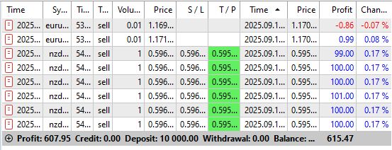
So far, the system's accuracy on the test segment is around 64-65%, while the average profit is much higher than the average loss.

Here is what we managed to get in a few days of trading:

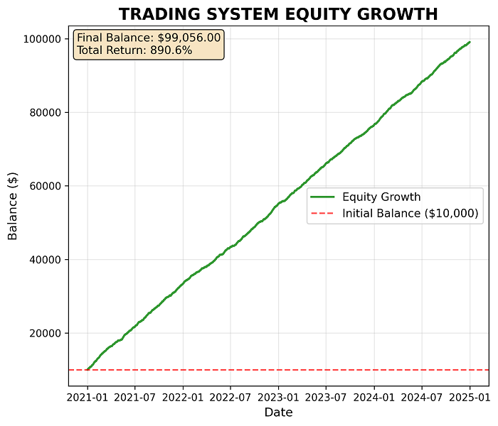
Simulations of profitability with a given win rate and risk for a portfolio of positions and for a single position separately are also very encouraging:

However, I do not really trust homemade Python testers, so I will either have to test the system extensively in real trading or rewrite the logic in MQL5 to gain access to a powerful strategy tester with a real tick database and requote emulation.

Full port to MQL5: An architectural revolution

The Python-MetaTrader 5 hybrid architecture has fundamental speed limitations. A full port to MQL5 will require the creation of our own machine learning libraries. Key modules include high-performance matrix operations for XGBoost, a gradient boosting implementation with native optimization for the x64 architecture, and an adapted version of Gaussian Mixture Models for feature clustering. This is a technically challenging task, but it will eliminate all API latency and provide a 10-50x performance boost.

Next-generation graphical interface

It is planned to create a full-fledged real-time GUI system with a modular architecture. The dashboard will display the current positions of all instruments, real-time P&L, risk limit usage, and the status of each trading flow. A critical component will be the dynamic parameter management module — the ability to change TOTAL_PORTFOLIO_RISK, model thresholds, and time horizons without restarting the system. The alert system will include notifications about daily loss limits being exceeded, abnormal model signals, and loss of connection with the broker.

A high-level risk manager: A quantum leap in portfolio management

The current risk management system looks primitive compared to the planned one. The new risk manager will analyze correlations between instruments in real time, using rolling windows of varying lengths. Value-at-Risk calculations based on Monte Carlo simulations will predict potential portfolio losses with varying levels of probability. The dynamic hedging system will automatically open offsetting positions when correlation risks are exceeded.

Multithreaded training: An army of models

The transition to massively parallel model training will be revolutionary. Each CPU thread will test different combinations of XGBoost hyperparameters, training periods, and feature sets. The system will automatically select the best model for each time period based on out-of-sample results. An ensemble of Random Forest, SVM, neural networks, and LightGBM will form a meta-model that outperforms any single implementation.

GAN for generating 25-year datasets: Synthetic market history

The most ambitious plan is to use Generative Adversarial Networks to create synthetic 25-year price series of major currency pairs. GAN will be trained on real historical data, then generate huge datasets that preserve the statistical properties of real markets: volatility clustering, fat-tailed distributions, autocorrelations. This will solve the problem of lack of data for deep learning.

An ensemble of 100 specialized models: Time-price space segmentation

The culmination will be the creation of an ensemble of 100 models, each responsible for its own "section" of market conditions. Each model will be trained on data from a specific regime: high volatility, sideways movement, strong trends, news periods, pre-holiday sessions. Such regimes can be identified, for example, through feature clustering, Markov chains, or SSM-based approaches. BaggingClassifier for each model will provide additional stability. The meta classifier will determine the current market regime with extremely high accuracy and activate the corresponding specialized models. This architecture will enable unprecedented forecast accuracy, adapting to any market conditions in real time.

Google Cloud Platform Integration: The computing power of 1,000-core supercomputers

Local computing resources become a bottleneck in implementing such ambitious plans. Google Cloud Platform provides the solution through direct integration with the Python API. The google-cloud-compute library allows programmatic creation of virtual machines with hundreds of CPU cores and terabytes of memory for parallel model training.

from google.cloud import compute_v1
from google.cloud import storage

# Creating a high-performance cluster
instance_client = compute_v1.InstancesClient()
operation = instance_client.insert(
    project="trading-ai-project",
    zone="us-central1-a", 
    instance_resource={
        "name": "trading-cluster-node",
        "machine_type": "zones/us-central1-a/machineTypes/c2-standard-60",
        "scheduling": {"preemptible": True}  # Cost reduction by 5 times
    }
)

AI Platform Training enables distributed training of XGBoost and neural networks on dozens of machines simultaneously. Cloud Storage provides instant access to petabytes of historical data. BigQuery ML integrates directly with trading algorithms to analyze patterns in real time.

A critical advantage is autoscaling of computing resources. During periods of model retraining, the system automatically launches hundreds of instances, and during quiet periods, it reduces them to a minimum, optimizing costs. Preemptible instances reduce computation costs by a factor of 5, making training our future highly complex models economically feasible.

Conclusion

In this article, we took the first steps towards creating a multi-threaded trading robot using machine learning methods. The architecture considered covers the entire path from data collection and augmentation to feature generation, clustering, training of XGBoost models and integration of portfolio risk management. We saw how the separation of roles between Python and MetaTrader 5 allows us to leverage the best of both worlds: the flexibility and rich ecosystem of Python libraries for machine learning, and the robustness of MetaTrader 5 for real-time trading execution.

However, this is only the first part of the series. In future publications, I plan to cover issues of porting the system to MQL5, developing a graphical interface, integrating with cloud services, using GANs to generate synthetic datasets, and building ensembles of specialized models. These steps will significantly expand the scale and improve the efficiency of the trading robot, paving the way for its full implementation.