Digital Signal Processing for Traders (Part 2): The Dominant Cycle, MAMA, and a Regime-Switching Expert Advisor

Contents

1. Introduction
2. Measuring the dominant cycle: the Hilbert transform
3. MAMA: a moving average that adapts to phase
4. The regime thesis: two markets, two playbooks
5. Building the regime-switching Expert Advisor
6. Edge cases and pitfalls
7. Testing in the Strategy Tester
8. Conclusion

Introduction

In Part 1 we took John F. Ehlers' engineering view of the market seriously. A price chart is a signal: a mixture of fast noise, a tradable cycle in the middle, and a slow trend baseline. We built a single-source-of-truth library, EhlersDSP.mqh, and inside it the Super Smoother (a low-lag low-pass filter), the Roofing Filter (a high-pass filter and the Super Smoother, cascaded to isolate the tradable band), and the Even Better Sinewave (a cycle oscillator whose railing behavior flags trend mode). That foundation is necessary but not sufficient. Seeing that price is trending or cycling is useful, but it does not tell you how to adapt a strategy's parameters to the market's current rhythm.

That gap is the concrete problem this part solves. Fixed-length averages and static oscillator settings inevitably miss the mark: they lag during accelerations and turn noisy during slowdowns, because the market's dominant rhythm breathes rather than holding still. What you need is a reproducible, code-level measurement of the dominant period (in bars), a way to turn that measurement into an adaptive moving average, and a self-contained regime-switching Expert Advisor that consumes those modules without relying on drawn indicator state or an iCustom handle. The implementation constraints are explicit and cross-cutting, not incidental: every decision is made on closed bars only, filters are replayed from history on each new bar, and every module exposes clear, testable accessors, such as Ready(), Value(), InPhase() and Quadrature(), so the EA can consume them deterministically.

Part 2 delivers exactly that, as three modules chained measurement to adaptation to application. First, a Hilbert-transform homodyne CyclePeriod engine that clamps and double-smooths the dominant-period estimate. Second, a faithful MAMA and FAMA implementation driven by the phase that engine exposes. Third, a regime-switching EA that classifies mode from the Even Better Sinewave and applies separate playbooks for trend and cycle, all built from the same shared DSP include and tested in the Strategy Tester on real ticks. The aim is reproducible engineering, not an out-of-the-box profitable system: you get modules that compile, run, and expose stable interfaces, plus the rules and caveats needed to validate them yourself. The mathematics stays honest but practical: you will see the exact formulas and coefficients Ehlers published, with enough explanation to trust the code, but we will not derive the Hilbert transform from first principles.

A note on scope and honesty. Everything here is built, compiled, and tested. The Strategy Tester figures in the testing section come from a real run on EURUSD M30 with 100% real ticks, and the balance curve is that run's own report; nothing is invented. That said, the result is a modest, unoptimized demonstration that the regime logic behaves as designed, not a finished, profitable trading system and not a recommendation to trade. The point of this series is the engineering, not a profit claim. Reproduce the test on your own terminal and your own symbol before you draw any conclusions.

Measuring the dominant cycle: the Hilbert transform

Every adaptive tool in Ehlers' toolkit rests on one measurement: how long is the cycle that currently dominates price? If the market is swinging with a roughly 20-bar rhythm, an oscillator tuned to 20 bars reads it cleanly, while one tuned to 10 or 40 does not. The trouble is that this dominant period is not constant. It breathes, stretching in quiet markets and compressing in fast ones, so it has to be measured continuously rather than assumed. That measurement is the job of the CyclePeriod class, and it is the engine that MAMA will reuse in the next section.

The idea, without the derivation. Think of the cycle component of price as a wave. At any instant a wave has a phase, an angle on the circle that tells you where in its swing it is: rising through zero, at the top, falling through zero, at the bottom. If you could read that phase on every bar, then the amount the phase advances from one bar to the next tells you the frequency, and the frequency inverted is the period. So measuring the dominant cycle reduces to measuring how fast the phase is turning.

To read phase you need two versions of the wave: the wave itself, called the in-phase component, and a copy shifted by exactly 90 degrees, called the quadrature component. With both in hand, the phase is just the arctangent of quadrature over in-phase, exactly the way you would read an angle from its sine and cosine. The device that produces a 90-degree-shifted copy of a signal is the Hilbert transform, and Ehlers approximates it with a short 7-tap filter. Fig. 1 shows the pieces and how they connect.

Fig. 1. The homodyne discriminator. Price is smoothed and detrended, split into an in-phase and a 90-degree quadrature component by the Hilbert filter, and the rate at which the combined phase turns is converted into the dominant-cycle period in bars.

The full method is Ehlers' homodyne discriminator. The word homodyne comes from radio: you multiply the signal by a delayed copy of itself to extract the beat frequency, and here the beat frequency is precisely the rate the phase is turning. The steps are as follows. Smooth the price, then detrend it with the Hilbert filter to obtain a near zero-mean wave. Produce the in-phase and quadrature components, advance them by 90 degrees, and recombine them to sharpen the estimate. Finally, multiply the current components by the previous bar's values to obtain the discriminator's real and imaginary parts. The angle of that complex number is the phase step, and the period follows.

Rather than paraphrase, here is the plain-language algorithm the class runs on every bar, so a reader who does not follow the trigonometry can still follow the logic:

1. Smooth the raw price with a short 4-bar weighted average to take the edge off single-bar noise.
2. Detrend it: apply the 7-tap Hilbert filter to the smoothed price, producing a near-zero-mean wave.
3. From the detrended wave, form the in-phase component (I1) and, with the Hilbert filter again, the quadrature component (Q1).
4. Advance the phase of I1 and Q1 by 90 degrees and recombine to get sharper I2 and Q2, then smooth them.
5. Homodyne: multiply I2, Q2 against the previous bar's values to get the real and imaginary parts, and smooth.
6. The dominant period is 2*pi divided by the phase step (the arctangent of imaginary over real).
7. Clamp the period so it cannot jump more than 50% bar-to-bar or leave the 6-to-50-bar band, then smooth it twice.

The one taxing part is the Hilbert filter itself, and it is small enough to state in full. Ehlers uses a fixed 7-tap finite-impulse-response filter with the weights 0.0962 and 0.5769, and then multiplies the result by a frequency-correction factor that depends on the current period estimate. Because we apply that same filter to four different signals in the discriminator, we write it once as a private helper:

//--- Ehlers' 7-tap Hilbert FIR with the .0962/.5769 weights,
//--- frequency-corrected by (.075*Period + .54).
double            Hilbert(const SignalHistory &s, const double period) const
  {
   return((0.0962 * s[0] + 0.5769 * s[2] - 0.5769 * s[4] - 0.0962 * s[6])
          * (0.075 * period + 0.54));
  }

Notice that it reads samples at indices 0, 2, 4 and 6, that is, the current bar and every second bar back to six bars ago. That even-spaced, antisymmetric tap pattern is what produces the 90-degree phase shift. The (0.075 * period + 0.54) factor is Ehlers' correction: the raw filter's gain varies with frequency, and this term compensates so the amplitude stays consistent as the measured period changes. It uses the previous bar's period estimate, which is why the class threads prevPeriod through every call. Here is the whole Update() method, which walks the seven steps above in order:

//--- feed price (typically (H+L)/2); returns smoothed period (bars)
double            Update(const double price)
  {
   m_price.Push(price);
   double prevPeriod = (m_count > 0 ? m_period[0] : 0.0);

   //--- 4-bar weighted smoother
   double smooth = price;
   if(m_price.Ready(4))
      smooth = (4.0 * m_price[0] + 3.0 * m_price[1] + 2.0 * m_price[2] + m_price[3]) / 10.0;
   m_smooth.Push(smooth);

   //--- Detrender, in-phase (I1) and quadrature (Q1) components
   double detr = 0.0, q1 = 0.0, i1 = 0.0;
   if(m_smooth.Ready(7))
     {
      detr = Hilbert(m_smooth, prevPeriod);
     }
   m_detr.Push(detr);
   if(m_detr.Ready(7))
     {
      q1 = Hilbert(m_detr, prevPeriod);
      i1 = m_detr[3];
     }
   m_q1.Push(q1);
   m_i1.Push(i1);

   //--- advance phase of I1,Q1 by 90 deg (jI, jQ) and combine
   double jI = 0.0, jQ = 0.0;
   if(m_i1.Ready(7))
      jI = Hilbert(m_i1, prevPeriod);
   if(m_q1.Ready(7))
      jQ = Hilbert(m_q1, prevPeriod);

   double i2 = i1 - jQ;
   double q2 = q1 + jI;
   //--- smooth I2,Q2 (.2/.8)
   if(m_count > 0)
     {
      i2 = 0.2 * i2 + 0.8 * m_i2[0];
      q2 = 0.2 * q2 + 0.8 * m_q2[0];
     }
   m_i2.Push(i2);
   m_q2.Push(q2);

   //--- homodyne discriminator: Re/Im of I2,Q2 against prior bar
   double re = i2 * (m_count > 0 ? m_i2[1] : 0.0) + q2 * (m_count > 0 ? m_q2[1] : 0.0);
   double im = i2 * (m_count > 0 ? m_q2[1] : 0.0) - q2 * (m_count > 0 ? m_i2[1] : 0.0);
   if(m_count > 0)
     {
      re = 0.2 * re + 0.8 * m_re[0];
      im = 0.2 * im + 0.8 * m_im[0];
     }
   m_re.Push(re);
   m_im.Push(im);

   //--- period from the beat-note angle, with Ehlers' clamps
   double period = prevPeriod;
   if(im != 0.0 && re != 0.0)
      period = 2.0 * EHLERS_PI / MathArctan(im / re); // 360/atan(deg) -> 2PI/atan(rad)
   if(prevPeriod > 0.0)
     {
      if(period > 1.5 * prevPeriod)
         period = 1.5 * prevPeriod;
      if(period < 0.67 * prevPeriod)
         period = 0.67 * prevPeriod;
     }
   if(period < 6.0)
      period = 6.0;
   if(period > 50.0)
      period = 50.0;
   if(m_count > 0)
      period = 0.2 * period + 0.8 * m_period[0];
   m_period.Push(period);

   double smoothP = period;
   if(m_count > 0)
      smoothP = 0.33 * period + 0.67 * m_smoothP[0];
   m_smoothP.Push(smoothP);

   m_count++;
   return(smoothP);
  }

Three details in that code repay a close look, because they are where a careless port goes wrong and where the class earns its robustness.

The clamps are not cosmetic. The raw period from the arctangent is noisy and occasionally nonsensical, so Ehlers imposes three limits in sequence: it may not change by more than 50% from the previous bar (1.5 and 0.67 are the up and down factors), and it must stay inside the 6-to-50-bar band that covers every tradable cycle. Without these, a single bad bar would throw the period to an absurd value that the downstream smoothing would then take many bars to shake off. The clamps keep the estimate on a short leash.

The double smoothing at the end is deliberate. The period is first blended 0.2/0.8 with its own previous value, then blended again 0.33/0.67 into smoothP, which is what the class returns. Two stages of exponential smoothing turn a jittery raw measurement into the slow, stable line you want feeding an adaptive average; a period estimate that jumps around every bar would make MAMA useless.

The public accessors at the bottom of the class are what let MAMA reuse this engine without recomputing anything:

double            Value()       const { return(m_smoothP[0]); }
double            RawPeriod()   const { return(m_period[0]); }
double            InPhase()     const { return(m_i1[0]); }
double            Quadrature()  const { return(m_q1[0]); }
bool              Ready()       const { return(m_count >= 7); }

Value() hands back the smoothed period for anyone who wants the cycle length, and InPhase() and Quadrature() expose the raw I1 and Q1 components. MAMA needs those two to compute phase directly, so instead of duplicating the entire discriminator inside MAMA, we expose them here and let MAMA read them. That is the same single-source-of-truth discipline from Part 1, applied within the library itself.

The indicator. With the class doing the work, the dominant-cycle indicator is thin. It declares one buffer, instantiates one CyclePeriod, and, exactly as in Part 1, re-initializes and replays the whole series on every OnCalculate because a stateful IIR filter cannot be resumed from the middle. The only new touch is the fixed vertical scale, so the period reads directly in bars against a stable axis.

//+------------------------------------------------------------------+
//|                                        EhlersCyclePeriod.mq5     |
//|   Dominant-cycle period (bars) via the Hilbert homodyne          |
//|   discriminator. The measurement engine behind MAMA.             |
//+------------------------------------------------------------------+
#property copyright "Adeolu Kayode"
#property strict
#property indicator_separate_window
#property indicator_buffers 1
#property indicator_plots   1

#property indicator_label1  "DominantCycle"
#property indicator_type1   DRAW_LINE
#property indicator_color1  clrOrange
#property indicator_width1  2
#property indicator_minimum 0
#property indicator_maximum 55

#include <Ehlers/EhlersDSP.mqh>

double       PeriodBuffer[];
CyclePeriod  g_cycle;

//+------------------------------------------------------------------+
//| Custom indicator initialization function                         |
//+------------------------------------------------------------------+
int OnInit()
  {
   SetIndexBuffer(0, PeriodBuffer, INDICATOR_DATA);
   IndicatorSetString(INDICATOR_SHORTNAME, "Ehlers Dominant Cycle");
   IndicatorSetInteger(INDICATOR_DIGITS, 1);
   return(INIT_SUCCEEDED);
  }
//+------------------------------------------------------------------+
//| Custom indicator iteration function                              |
//+------------------------------------------------------------------+
int OnCalculate(const int rates_total,
                const int prev_calculated,
                const datetime &time[],
                const double &open[],
                const double &high[],
                const double &low[],
                const double &close[],
                const long &tick_volume[],
                const long &volume[],
                const int &spread[])
  {
   if(rates_total < 16)
      return(0);

   g_cycle.Init();
   for(int i = 0; i < rates_total; i++)
     {
      double price = (high[i] + low[i]) / 2.0;
      double p = g_cycle.Update(price);
      PeriodBuffer[i] = (g_cycle.Ready() ? p : EMPTY_VALUE);
     }
   return(rates_total);
  }

The g_cycle.Ready() ? p : EMPTY_VALUE guard is the same warm-up discipline from Part 1: until the discriminator has its seven samples there is no meaningful period, so we write EMPTY_VALUE and the terminal draws nothing rather than a misleading flat line. On the chart the dominant-cycle line drifts slowly between roughly 10 and 40 bars, sinking when the market speeds up into short swings and rising when the swings lengthen. It is not a signal you trade directly; it is the number that every adaptive tool downstream needs.

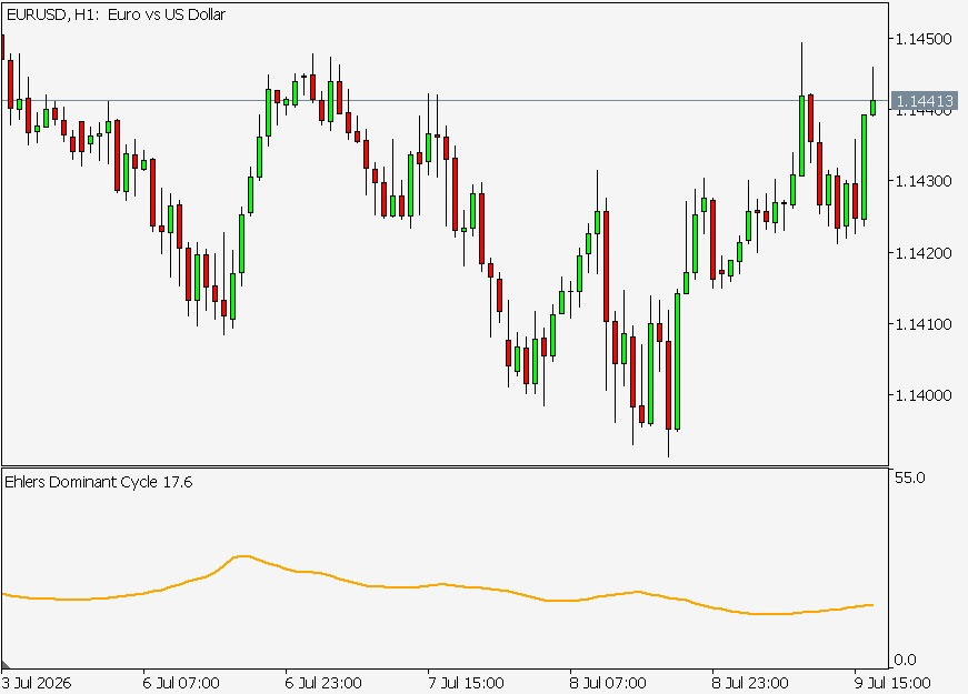
Fig. 2. The dominant-cycle period (lower subwindow) measured on EURUSD. The line reports the length in bars of the swing currently dominating price, drifting within the 6-to-50-bar band as the market's rhythm stretches and compresses.

MAMA: a moving average that adapts to phase

Ehlers introduced the MESA Adaptive Moving Average in a 2001 paper with a pointed observation: the trouble with every fixed-length moving average is that the correct length keeps changing. A 20-bar average is too slow when the market is trending hard and too fast when it is chopping sideways. The fix is an average whose responsiveness adapts, fast when it should be fast, slow when it should be slow, and MAMA drives that adaptation directly from the phase we just learned to measure.

The mechanism is elegant. A standard exponential moving average has a smoothing constant, alpha, between 0 and 1: a large alpha weights the newest price heavily and reacts fast, a small alpha reacts slowly. MAMA makes alpha adaptive by tying it to the rate of change of phase. When the market trends, its phase advances slowly and steadily, so alpha is allowed to rise and the average tracks price closely. When the market cycles, the phase spins quickly, so alpha is forced down and the average smooths hard. In Ehlers' words, MAMA "adapts to the rate change of phase as measured by the Hilbert Transform Discriminator":

"The adaptation is based on the rate change of phase as measured by the Hilbert Transform Discriminator I described in my May and June 2000 Stocks & Commodities articles. When the phase is changing rapidly, the alpha is made larger to produce very little smoothing. When the phase is changing slowly, alpha is made smaller for more smoothing."

— Source: John F. Ehlers, "MESA Adaptive Moving Averages" (MESA Software)

Because the phase and its components already live inside CyclePeriod, the MAMA class does not recompute any of the Hilbert machinery. It contains a CyclePeriod, drives it with the price on each bar, and reads back the in-phase and quadrature components to compute the phase itself. The whole class is short:

//+------------------------------------------------------------------+
//  MAMA / FAMA — MESA Adaptive Moving Average and its follower.     |
//  alpha adapts to the rate of change of phase (DeltaPhase) from    |
//  the Hilbert discriminator. Fast in trends, slow in congestion.   |
//  Ref: MESA "MAMA" paper (2001), FastLimit .5 / SlowLimit .05.     |
//+------------------------------------------------------------------+
class MAMA
  {
private:
   CyclePeriod       m_cycle;       // reuse the discriminator engine
   SignalHistory     m_phase;       // instantaneous phase (need 1 back for DeltaPhase)
   double            m_mama;        // MAMA value (adaptive moving average)
   double            m_fama;        // FAMA value (the slower follower line)
   double            m_fastLimit;   // upper bound on adaptive alpha (trend speed)
   double            m_slowLimit;   // lower bound on adaptive alpha (congestion speed)
   int               m_count;       // samples processed so far (for warm-up)
public:
   void              Init(const double fastLimit = 0.5, const double slowLimit = 0.05)
     {
      m_cycle.Init();
      m_phase.Init(2);
      m_fastLimit = fastLimit;
      m_slowLimit = slowLimit;
      m_mama = 0.0;
      m_fama = 0.0;
      m_count = 0;
     }
   //--- feed price (typically (H+L)/2)
   void              Update(const double price)
     {
      m_cycle.Update(price);                 // drives I1/Q1 internally

      double i1 = m_cycle.InPhase();
      double q1 = m_cycle.Quadrature();

      //--- instantaneous phase (degrees->radians handled by atan)
      double phase = (m_count > 0 ? m_phase[0] : 0.0);
      if(i1 != 0.0)
         phase = MathArctan(q1 / i1);
      double deltaPhase = (m_count > 0 ? (m_phase[0] - phase) : 1.0);
      if(deltaPhase < 1e-8)
         deltaPhase = 1e-8;   // Ehlers: DeltaPhase = max(.,1) in DEG; guard div0 in RAD
      m_phase.Push(phase);

      double alpha = m_fastLimit / deltaPhase;
      if(alpha < m_slowLimit)
         alpha = m_slowLimit;
      if(alpha > m_fastLimit)
         alpha = m_fastLimit;

      if(m_count == 0)
        {
         m_mama = price;
         m_fama = price;
        }
      else
        {
         m_mama = alpha * price + (1.0 - alpha) * m_mama;
         m_fama = 0.5 * alpha * m_mama + (1.0 - 0.5 * alpha) * m_fama;
        }
      m_count++;
     }
   double            Mama() const { return(m_mama); }
   double            Fama() const { return(m_fama); }
   bool              Ready() const { return(m_cycle.Ready()); }
  };

Read the middle of Update() against the mechanism. The phase is MathArctan(q1 / i1), the angle formed by the quadrature and in-phase components. deltaPhase is how much that angle moved since the previous bar, which is the rate of change of phase Ehlers ties alpha to. Then alpha = m_fastLimit / deltaPhase: a large phase step (fast cycling) makes alpha small, a small phase step (steady trending) makes alpha large, exactly the adaptation we want. The two bounds, FastLimit and SlowLimit, cap alpha so it can never react faster than a roughly two-bar average or slower than a twenty-bar one; their defaults of 0.5 and 0.05 are Ehlers' own.

The last two lines produce the two plotted values. m_mama is the adaptive average itself. m_fama, the Following Adaptive Moving Average, is a second average that follows MAMA at half its alpha, so it always lags MAMA slightly. That lag is the point: when MAMA crosses above FAMA the short-term average has turned up faster than its follower, a bullish signal, and a cross below is bearish. The two lines together give a self-contained trend direction, which is exactly what the Expert Advisor will read in trend mode.

Not the built-in AMA. MetaTrader 5 ships an iAMA, but that is Kaufman's Adaptive Moving Average, which adapts to an efficiency ratio (how directional recent price has been), not Ehlers' MAMA, which adapts to the Hilbert phase. They are different indicators with different math. The class here is Ehlers' MAMA and does not call iAMA.

The indicator. The MAMA indicator plots both lines on the price chart, MAMA solid and FAMA dotted, so the crossovers are visible directly against price. It exposes the two limits as inputs and follows the same replay-the-whole-series structure. The one point worth showing is how both buffers are filled together and gated on Ready():

int OnCalculate(const int rates_total,
                const int prev_calculated,
                const datetime &time[],
                const double &open[],
                const double &high[],
                const double &low[],
                const double &close[],
                const long &tick_volume[],
                const long &volume[],
                const int &spread[])
  {
   if(rates_total < 16)
      return(0);

   g_mama.Init(InpFastLimit, InpSlowLimit);
   for(int i = 0; i < rates_total; i++)
     {
      double price = (high[i] + low[i]) / 2.0;
      g_mama.Update(price);
      if(g_mama.Ready())
        {
         MamaBuffer[i] = g_mama.Mama();
         FamaBuffer[i] = g_mama.Fama();
        }
      else
        {
         MamaBuffer[i] = EMPTY_VALUE;
         FamaBuffer[i] = EMPTY_VALUE;
        }
     }
   return(rates_total);
  }

On the chart, MAMA hugs price tightly through trends and flattens out through congestion, visibly changing its own speed, which no fixed moving average can do. FAMA trails it, and the points where the two cross mark the changes of direction the strategy will use.

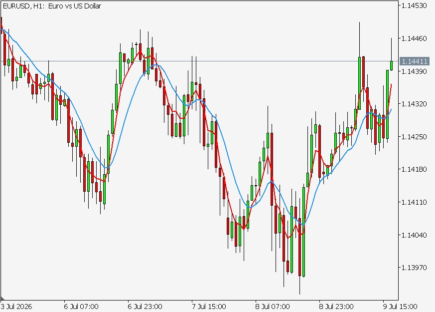
Fig. 3. MAMA (solid) and FAMA (dotted) on EURUSD. MAMA speeds up to track trends and slows through congestion; the crossings of the two lines mark the direction changes the Expert Advisor reads in trend mode.

The regime thesis: two markets, two playbooks

We now have every component the strategy needs, so before we write the Expert Advisor it is worth stating plainly the idea that ties them together, because it is the reason the whole series was built this way. Ehlers' central thesis is that the market is, at any moment, in one of two modes and only two: it is either cycling, swinging rhythmically around a stable value, or trending, moving persistently in one direction. These are not just two chart patterns; they demand opposite trading behavior. In a cycle, the winning move is mean reversion: sell the highs, buy the lows, because price keeps returning to the middle. In a trend, mean reversion is exactly how accounts are destroyed, because fading a trend means betting against the one thing that is working, and the winning move is to follow the trend until it ends.

The catch, and the reason most indicators fail, is that a tool built for one mode is actively harmful in the other. A swing oscillator that prints reliable buy and sell signals in a range will scream "overbought" and pin there for the whole of a trend, feeding you losing fade after losing fade. A trend-following moving average that rides a strong move beautifully will whipsaw you to pieces in a range. The single most valuable thing a system can do, then, is not to trade better in either mode, but to know which mode it is in and switch playbooks accordingly.

That is precisely what our tools measure. From Part 1, the Even Better Sinewave rails near +1 or -1 when the market trends and oscillates between the level lines when it cycles, so its railing is a direct mode detector. From this part, MAMA and FAMA give a clean trend direction, and the dominant cycle gives the rhythm. The Expert Advisor combines them along the lines of Fig. 4: read the Even Better Sinewave to decide the mode, then hand control to the matching playbook, mean reversion off the sinewave in cycle mode, trend following off MAMA and FAMA in trend mode.

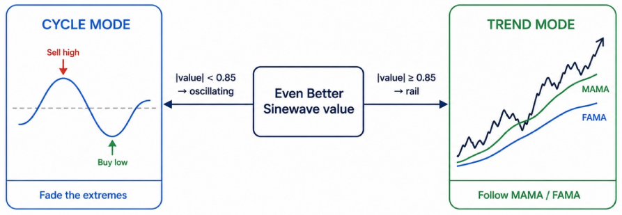
Fig. 4. The regime switch. The Even Better Sinewave's value selects the mode: when it rails past the trend threshold the EA follows MAMA and FAMA; when it oscillates below the threshold the EA fades the sinewave's extremes back toward zero.

This is a deliberately simple rule, and that is on purpose. The goal of the article is to show the DSP tools driving a real decision end to end, not to present a heavily engineered strategy. A single threshold on the sinewave selects the mode, and each mode runs the most obvious version of its playbook. Everything subtle in the system lives in the filters we already built; the EA on top of them is intentionally readable.

Building the regime-switching Expert Advisor

The Expert Advisor, EhlersRegimeEA.mq5, pulls its math from the same include the indicators use, so there is no iCustom, no indicator handles, and no chance of the EA's numbers drifting from the indicators' numbers. It computes the filters itself, in its own process, from the same class library. Its header states the strategy in full, and it is worth reading because it is the specification the rest of the file implements:

//+------------------------------------------------------------------+
//|                                            EhlersRegimeEA.mq5    |
//|   Regime-switching EA built on Ehlers' DSP toolkit.              |
//|                                                                  |
//|   Ehlers' central thesis: the market is always in one of two     |
//|   modes. This EA measures the mode with the Even Better Sinewave |
//|   and trades each mode on its own terms:                         |
//|                                                                  |
//|     CYCLE MODE  (EBSW oscillating, |EBSW| not railed)            |
//|        -> mean-reversion: fade the sinewave extremes.            |
//|     TREND MODE  (EBSW railed near +/-1)                          |
//|        -> trend-following: trade in the MAMA/FAMA direction.     |
//|                                                                  |
//|   All DSP math comes from the shared include (no iCustom).       |
//+------------------------------------------------------------------+
#property copyright "Adeolu Kayode"
#property strict

#include <Ehlers/EhlersDSP.mqh>
#include <Trade/Trade.mqh>

It includes the standard CTrade class for order handling, which keeps the trading plumbing out of our way. The inputs expose the parameters of both the filters and the strategy:

//--- inputs -------------------------------------------------------//
input double   InpFastLimit   = 0.5;    // MAMA fast limit
input double   InpSlowLimit   = 0.05;   // MAMA slow limit
input double   InpDuration    = 40.0;   // EBSW high-pass duration
input double   InpRailLevel   = 0.85;   // |EBSW| >= this => trend mode
input double   InpCycleEntry  = 0.70;   // cycle-mode fade trigger
input double   InpLots        = 0.10;   // fixed lot size
input int      InpStopPoints  = 400;    // stop loss (points); 0 = none
input int      InpTakePoints  = 800;    // take profit (points); 0 = none
input ulong    InpMagic       = 20260621;
input int      InpSlippage    = 20;

The two limits tune MAMA, the duration tunes the Even Better Sinewave, and the two threshold inputs are the strategy's only real knobs. InpRailLevel (0.85) is the sinewave value at or beyond which we call the market trending; InpCycleEntry (0.70) is how far the sinewave must swing before we treat an extreme as a fade opportunity in cycle mode. The rest are ordinary trade-management inputs: a fixed lot, an optional stop and target in points, a magic number so the EA only ever manages its own positions, and a slippage tolerance.

The globals instantiate one of each filter and hold the per-bar state the decision logic reads:

//--- globals ------------------------------------------------------//
MAMA                g_mama;
EvenBetterSinewave  g_ebsw;
CTrade              g_trade;
datetime            g_lastBarTime = 0;

//--- per-bar computed state (rebuilt each new bar) ----------------//
double  g_curEBSW  = 0.0;
double  g_prevEBSW = 0.0;
double  g_mamaVal  = 0.0;
double  g_famaVal  = 0.0;
bool    g_ready    = false;

Rebuilding the filter state on each bar. Here is the crux of running stateful IIR filters inside an EA rather than an indicator. In an indicator, OnCalculate hands us the whole price array and we replay the filters across it. An EA has no such array; it is called tick by tick. But the filters still cannot be resumed from the middle, they only make sense fed every bar in order from the start, so on each new bar we do the same thing the indicator does: pull a slab of recent history and replay the filters across it from scratch. That is the job of ComputeState():

//+------------------------------------------------------------------+
//| Replay the DSP filters over closed bars to get current state.    |
//| Stateful IIR filters can't be resumed mid-series, so we rebuild  |
//| from history on each new bar. We use only CLOSED bars (index 1+).|
//+------------------------------------------------------------------+
bool ComputeState()
  {
   int bars = Bars(_Symbol, _Period);
   if(bars < 64)
      return(false);

//--- pull enough history; cap for speed
   int need = MathMin(bars - 1, 1500);
   MqlRates rates[];
   ArraySetAsSeries(rates, false);
   int copied = CopyRates(_Symbol, _Period, 1, need, rates); // start at 1 => closed bars only
   if(copied <= 16)
      return(false);

   g_mama.Init(InpFastLimit, InpSlowLimit);
   g_ebsw.Init(InpDuration);

   double prevE = 0.0, curE = 0.0;
   for(int i = 0; i < copied; i++)
     {
      double price = (rates[i].high + rates[i].low) / 2.0;
      g_mama.Update(price);
      prevE = curE;
      curE  = g_ebsw.Update(price);
     }

   if(!g_mama.Ready() || !g_ebsw.Ready())
      return(false);

   g_prevEBSW = prevE;
   g_curEBSW  = curE;
   g_mamaVal  = g_mama.Mama();
   g_famaVal  = g_mama.Fama();
   return(true);
  }

Three decisions in this function matter. First, the CopyRates call starts at index 1, not 0, so it copies only closed bars and never the forming bar. The current bar's high and low are still moving, and feeding a half-formed bar into a recursive filter would make the EBSW value flicker within the bar and produce different decisions on different ticks. By replaying only closed bars, the state is identical on every tick of a given bar, so the decision is stable. Second, the history is capped at 1500 bars with MathMin. A recursive filter's memory of its distant past decays, so 1500 bars is far more than enough to reach the same state a full replay would, and it keeps the per-bar cost flat no matter how much history the chart holds. Third, the function refuses to act until both filters report Ready(), so the warm-up bars never generate a trade. The array is set non-series with ArraySetAsSeries(rates, false) so that index 0 is the oldest bar, which is the order the filters must be fed.

Acting once per bar. The decision logic lives in OnTick, but it must run only once per bar, on the close, not on every tick. The guard at the top enforces that:

//+------------------------------------------------------------------+
//| Decide and act once per new closed bar.                          |
//+------------------------------------------------------------------+
void OnTick()
  {
   datetime barTime = (datetime)SeriesInfoInteger(_Symbol, _Period, SERIES_LASTBAR_DATE);
   if(barTime == g_lastBarTime)
      return;                 // act on bar close only
   g_lastBarTime = barTime;

   if(!ComputeState())
      return;

   bool trendMode = (MathAbs(g_curEBSW) >= InpRailLevel);

   long posType;
   bool havePos = HasOpenPosition(posType);

The bar-time comparison is a standard MQL5 idiom: SeriesInfoInteger with SERIES_LASTBAR_DATE returns the open time of the most recent bar, and when it changes we know a new bar has opened, which means the previous one has just closed. We store it and return immediately on every subsequent tick of the same bar. Then we compute the state and read the single most important line: trendMode is true when the sinewave's magnitude has reached the rail level. That one boolean selects the playbook.

The trend-mode branch follows MAMA and FAMA:

 if(trendMode)
     {
      //--- TREND MODE: follow MAMA/FAMA. MAMA above FAMA => up-trend.
      bool up = (g_mamaVal > g_famaVal);
      if(!havePos)
         OpenTrade(up);
      else
        {
         //--- flip if the trend direction reversed
         bool posIsBuy = (posType == POSITION_TYPE_BUY);
         if(posIsBuy != up)
           {
            ClosePosition();
            OpenTrade(up);
           }
        }
     }

The direction is read straight from the two adaptive averages: MAMA above FAMA is an up-trend, MAMA below is a down-trend. With no position open, the EA enters in that direction. With a position already open, it does nothing unless the trend has flipped against it, in which case it closes and reverses. This is deliberately a stop-and-reverse trend follower; while the trend holds, it simply stays in.

The cycle-mode branch does the opposite, fading the sinewave's extremes:

 else
     {
      //--- CYCLE MODE: mean-revert. Fade sinewave extremes as they
      //--- turn back from the threshold toward zero.
      bool fadeShort = (g_prevEBSW >  InpCycleEntry && g_curEBSW <  g_prevEBSW);
      bool fadeLong  = (g_prevEBSW < -InpCycleEntry && g_curEBSW >  g_prevEBSW);

      if(!havePos)
        {
         if(fadeLong)
            OpenTrade(true);
         else
            if(fadeShort)
               OpenTrade(false);
        }
      else
        {
         //--- exit mean-reversion trade once the wave crosses zero
         bool posIsBuy = (posType == POSITION_TYPE_BUY);
         if(posIsBuy && g_curEBSW >= 0.0)
            ClosePosition();
         else
            if(!posIsBuy && g_curEBSW <= 0.0)
               ClosePosition();
        }
     }
  }

The fade logic is careful in a way worth pointing out. It does not sell the instant the sinewave is high; it waits for the sinewave to have been beyond the entry threshold and to have started turning back toward zero (g_curEBSW < g_prevEBSW for a short). That "past the threshold and now reversing" condition is what distinguishes a genuine cycle top, where the swing is rolling over, from the start of a trend, where the sinewave pushes to the rail and keeps going. The exit is simpler: a mean-reversion trade is closed once the sinewave crosses back through zero, because by then the swing has completed its move to the other side and there is no edge left in holding. The order-management helpers, OpenTrade, ClosePosition, HasOpenPosition, and the stop and target calculators, are ordinary CTrade wrappers, filtered by the magic number so the EA only ever touches its own trades; they are in the attached source and need no separate walkthrough.

Edge cases and pitfalls

This is the section that the documentation cannot give you, because every issue here comes from the specific act of running Ehlers' recursive filters inside a live trading program. Each of these is a place where the obvious approach is wrong and the code deliberately does something less obvious.

The full replay on every bar is not laziness, it is correctness. The instinct of any experienced MQL5 developer looking at ComputeState() is to optimize it: why recompute 1500 bars of filter output on every single bar when only one new bar has arrived? The answer is that there is no correct shortcut. These are infinite-impulse-response filters; today's output depends on a chain of previous outputs reaching back to the beginning of the series. To resume the computation for just the newest bar, you would need to have preserved the exact internal state of every filter, every ring buffer, every intermediate I, Q, Re, Im, and period value, at the previous bar. You could build that, but it multiplies the surface area for bugs enormously, and the moment one piece of saved state is wrong the filter output is silently corrupted from that bar on. Replaying from history is stateless between calls, impossible to get subtly wrong, and, because a recursive filter forgets its distant past, produces an output indistinguishable from a full replay. For the few hundred milliseconds it costs once per bar, it is the right trade.

The arctangent only sees two quadrants, and that is by design. Both the phase in MAMA and the period angle in the discriminator come from MathArctan, and it is worth being precise about what that function returns:

"MathArctan returns the arctangent of x in radians. The value returned is within the range of -π/2 to π/2 radians."

MQL5 Documentation: MathArctan

Because it takes a single ratio, MathArctan cannot distinguish an angle in one quadrant from the diagonally opposite one; a two-argument atan2 would resolve the full circle, but Ehlers' published formulas deliberately use the single-argument arctangent. The reason it works anyway is the layers of protection around it. The period estimate that comes out of the arctangent is immediately passed through the bar-to-bar clamps and then two stages of smoothing, so an occasional quadrant ambiguity is caught and averaged out long before it reaches MAMA or the trading logic. This is faithful to Ehlers' listings, and understanding it prevents a well-meaning "fix" to atan2 that would actually diverge from his published behavior. If you do experiment with atan2, treat it as a change to the algorithm, not a bug fix, and re-validate.

The division guards are load-bearing. Scattered through the classes are small conditions like if(im != 0.0 && re != 0.0) before the period division, if(i1 != 0.0) before the phase, and if(deltaPhase < 1e-8) deltaPhase = 1e-8 before the alpha division. In a recursive filter these are not defensive niceties, they are essential. A single division by zero produces a not-a-number, and because the filter feeds on its own past, that NaN propagates into every subsequent value and never clears. One unguarded edge case at bar 400 would poison the entire rest of the chart. Ehlers' EasyLanguage listings run in an environment that quietly tolerates these cases; a faithful MQL5 port has to make the guards explicit, and every one of them is there for a reason.

Acting on closed bars only. The EA makes decisions from the sinewave and MAMA values, and both are computed from closed bars, deliberately. If the EA read the forming bar, the median price feeding the filters would change with every tick, the EBSW value would wander within the bar, and the same bar could be classified as trending on one tick and cycling on the next, opening and closing trades in a flurry. Both the once-per-bar guard in OnTick and the start-at-index-1 in CopyRates exist to make each bar produce exactly one decision from settled data. This also means the EA is honest in backtesting: it uses no information from the still-forming bar, so a Strategy Tester result on this design is not inflated by look-ahead on the current bar.

The warm-up gate. Every class carries a Ready() method and a m_count that tracks how many samples it has seen, and nothing downstream trusts a filter until it reports ready. The discriminator needs seven samples before its Hilbert taps are all real; before that, reading its output would mean treating warm-up zeros as genuine measurements. The EA checks g_mama.Ready() and g_ebsw.Ready() and the indicators write EMPTY_VALUE during warm-up, so the first few bars of every run are correctly treated as "no signal yet" rather than a signal that happens to be zero. It is a small discipline that keeps the first trades from being made on noise.

Testing in the Strategy Tester

With the EA built, the honest question is whether the regime logic actually does something coherent on real data. To check, the EA was run in the MetaTrader 5 Strategy Tester on EURUSD, M30, with the "Every tick based on real ticks" model, over roughly five weeks of history. The parameters were the defaults shown earlier, deliberately unoptimized, because the aim is to see whether the mechanism behaves as designed, not to fit the best possible curve to this particular window. The test settings were:

Setting	Value
Symbol / timeframe	EURUSD, M30
Modeling	Every tick based on real ticks (100% history quality)
Period	2026.03.13 - 2026.04.17 (1200 bars)
Initial deposit / leverage	10 000, 1:500
Parameters	Defaults (FastLimit 0.5, SlowLimit 0.05, Duration 40, Rail 0.85, CycleEntry 0.70, 0.10 lot, 400/800 pt stop/target)

The headline outcome is that the strategy came through the test with a positive expectancy and a notably shallow drawdown. The full result set is below.

Metric	Value
Total net profit	180.50 (account in "profit in pips" mode, so 180.5 pips)
Profit factor	1.18
Sharpe ratio	2.25
Balance drawdown maximal	182.20 (1.79%)
Equity drawdown maximal	217.50 (2.13%)
Recovery factor	0.83
Expected payoff	0.89 per trade
Total trades	203
Profit trades / loss trades	94 (46.31%) / 109 (53.69%)
Long won % / short won %	52.04% / 40.95%
Average profit / average loss	12.68 / -9.28

Taken together, these numbers are consistent for such a simple, unoptimized rule. The profit factor of 1.18 means the strategy took out 1.18 units for every unit it gave back, a positive edge over 203 trades, which is a large enough sample that the result is not one or two lucky trades. The Sharpe ratio of 2.25 is genuinely good; it says the returns were smooth relative to their volatility, which is exactly what a regime filter is supposed to buy you, fewer of the violent swings that come from trading the wrong playbook. The clearest evidence of that smoothness is the drawdown: a maximal balance drawdown of just 1.79% on a 10,000 account is very shallow, and it is the number a risk-conscious reader should be most struck by. The strategy stayed out of deep trouble the whole way through.

The win rate deserves a word so it is not misread. At 46.31%, the strategy won fewer than half its trades, yet still finished ahead, and the reason is in the last row of the table: the average win (12.68) is larger than the average loss (-9.28). That is the signature of a system that cuts losers and lets winners run a little further, which is precisely what the 400/800-point stop-and-target ratio and the trend-following exit are built to do. A sub-50% win rate is not a weakness here; it is the expected shape of a favorable-payoff strategy. It is also worth noting that the long side (52.04% won) outperformed the short side (40.95%) over this particular window, a reminder that a five-week sample carries its own directional bias.

The balance curve makes the character of the run visible in one picture.

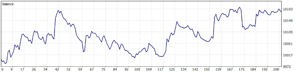
Fig. 5. The Strategy Tester balance curve. Equity climbs early, gives back part of the gain through a mid-test consolidation near the 100th trade, then recovers to close the run near its highs, ending up roughly 180 pips with the shallow drawdown reported above.

From the curve you can see the two faces of the strategy. The early rise and the late recovery are the trend-mode trades working, staying with directional moves; the choppy give-back in the middle third is the cost of cycle-mode fading during a stretch where the mode calls were less clean. That middle section is where the honest limits of a single-threshold regime switch show: a smarter mode filter, or an adaptive rail level, might have sat out that chop. The curve neither soars nor collapses, and for the purpose of this article that is the right result, it shows the DSP tools driving a coherent, risk-controlled strategy end to end.

Do not treat this as a validated trading system. This is one symbol, one timeframe, one five-week window, with default parameters and no walk-forward or out-of-sample testing. A positive profit factor and a good Sharpe on a single short sample are encouraging evidence that the mechanism works, not proof that it will be profitable going forward. Before risking anything, test it across multiple symbols and market conditions, run a walk-forward analysis, and account for your broker's real spread and commission. The value delivered here is the engineering, not this equity curve.

Conclusion

Across two parts we have closed the measurement to adaptation to application chain and followed Ehlers' claim that a price chart is a signal all the way from filter theory to a working, tested Expert Advisor. We saw how a dominant period is derived from the in-phase and quadrature components via the Hilbert homodyne discriminator, how that period and phase become an adaptive alpha for MAMA and FAMA, and how mode switching and trading logic on closed bars are built on top. Concretely, the article delivers three production-ready components, each with explicit behavior and interfaces:

1. CyclePeriod class and indicator. The Hilbert homodyne discriminator that returns a smoothed dominant period in bars, with hard clamps (6 to 50 bars, no more than 50% change bar-to-bar), double smoothing, and public accessors Value() (smoothed period), RawPeriod(), InPhase(), Quadrature() and Ready(). This is a stable, testable input for any adaptive module.
2. MAMA and FAMA implementation. An adaptive exponential average that reads the cycle engine's in-phase and quadrature components to compute instantaneous phase and its rate of change, converts that into an alpha bounded by FastLimit and SlowLimit, and exposes Mama(), Fama() and Ready(). It follows Ehlers' algorithm faithfully and includes the division and NaN guards essential for robustness.
3. Regime-switching Expert Advisor. A self-contained EA that replays closed-bar history on each new bar, rebuilds filter state with no iCustom, classifies mode from the Even Better Sinewave rail threshold, and runs two separate playbooks: trend (follow MAMA and FAMA) and cycle (fade EBSW extremes). It obeys the warm-up gate, acts once per closed bar, and is deterministic in backtests with no look-ahead.

The Strategy Tester run confirmed exactly what a regime filter should confirm: the mode classification stays stable on closed bars, there is no repainting, the warm-up gate behaves, and the whole apparatus runs coherently on real tick data with a positive edge and a shallow drawdown. The engineering lessons carry beyond this specific system. Replay filters from closed-bar history every bar and prefer correctness over micro-optimizations; compute state and act on closed bars only; protect every division and trigonometric step against NaN propagation; and keep a single source of truth, the shared EhlersDSP.mqh, so the indicators and the EA can never diverge. The "no iCustom" rule is not a stylistic detail but the mechanism behind that reproducibility: the EA owns its filter state instead of depending on another indicator's drawn, possibly redrawn, buffer.

Take the EA as a starting point rather than a finished product: the mode filter, the entry logic, and the exits are all deliberately simple, and each is an obvious place to extend. Recommended next steps are to validate across multiple instruments and timeframes, perform walk-forward and out-of-sample testing, and consider an adaptive rail or a mode-confidence metric if you want to reduce whipsaw in mixed regimes. The filters underneath the strategy are the part that is hard to get right, and those are now yours to build on.

File	Type	Description
EhlersDSP.mqh	Library	The full DSP class library: SignalHistory, SuperSmoother, RoofingFilter, CyclePeriod, MAMA, and EvenBetterSinewave.
EhlersRoofingFilter.mq5	Indicator	Roofing Filter (2-pole high-pass cascaded into a Super Smoother) plotted in a subwindow. Built in Part 1.
EhlersEvenBetterSinewave.mq5	Indicator	Even Better Sinewave oscillator with level lines, showing cycle swings and trend-mode railing. Built in Part 1.
EhlersCyclePeriod.mq5	Indicator	Dominant-cycle period (bars) via the Hilbert homodyne discriminator, plotted in a subwindow.
EhlersMAMA.mq5	Indicator	MESA Adaptive Moving Average (MAMA) and its follower FAMA, plotted on the price chart.
EhlersRegimeEA.mq5	Expert Advisor	Regime-switching EA: Even Better Sinewave selects cycle vs trend mode, then fades the sinewave (cycle) or follows MAMA/FAMA (trend).